PP 2017 09: The Atkinson Inequality Index in Multiagent Resource Allocation

The Atkinson Inequality Index

in Multiagent Resource Allocation

Sebastian Schneckenburger

Germany

sebastian.schneckenburger

@uni-tuebingen.de

Britta Dorn

Germany

britta.dorn

@uni-tuebingen.de

Ulle Endriss

The Netherlands

[email protected]

ABSTRACT

We analyse the problem of finding an allocation of resources in a multiagent system that is as fair as possible in terms of minimising inequality between the utility levels enjoyed by the individual agents. We use the well-known Atkin-son index to measure inequality and we focus on the dis-tributed approach to multiagent resource allocation, where new allocations emerge as the result of a sequence of lo-cal deals between groups of agents agreeing on an exchange of some of the items in their possession. Our results show that it is possible to design systems that provide theoreti-cal guarantees for optimal outcomes that minimise inequal-ity, but also that in practice there are significant compu-tational hurdles to be overcome: finding an optimal allo-cation is computationally intractable—independently of the approach chosen—and large numbers of potentially highly complex deals may be required under the distributed ap-proach. From a methodological point of view, while much work in multiagent resource allocation relies on combinato-rial arguments, here we use insights from basic calculus.

Keywords

Multiagent Resource Allocation; Fair Division; Inequality Indices

1.

INTRODUCTION

“What thoughtful rich people call the problem of poverty, thoughtful poor people call with equal justice a problem of riches.”

—Anthony B. Atkinson (1944 – 2017),Inequality [3]

Allocating resources to agents is one of the central tasks aris-ing in most multiagent systems [9]. This is true not only for systems of economic agents who need to share the value they have generated together, but also for distributed systems of problem-solving agents who need to share the computational resources available to them. What makes a ‘good’ alloca-tion heavily depends on the applicaalloca-tion at hand, but there is broad consensus in the multiagent systems research com-munity that, rather than coming up with newad hoccriteria for optimality for every new application, it is fruitful to base

Appears in:Proc. of the 16th International Conference on Autonomous Agents and Multiagent Systems (AAMAS 2017), S. Das, E. Durfee, K. Larson, M. Winikoff (eds.),

May 8–12, 2017, S˜ao Paulo, Brazil.

Copyright c2017, International Foundation for Autonomous Agents and Multiagent Systems (www.ifaamas.org). All rights reserved.

the design of a multiagent system on well-understood formal criteria originally proposed in the literature on social choice theory and welfare economics [20].

For instance, if an efficient allocation is sought, both the notion ofutilitarian social welfare, measuring quality in terms of the sum of the individual utilities, and the weaker notion ofPareto optimalityhave been found to be useful [26]. If fairness is a relevant design objective, there is a much wider range of concepts to choose from, several of which have been analysed in the literature on multiagent systems in some detail: e.g., egalitarian social welfare, measuring quality as utility of the worst-off agent, and its refinement theleximin-ordering [14, 6],Nash social welfare, measuring quality as the product of the individual utilities [24, 23], and theabsence of envy [17, 10]. However, fairness criteria based on measuring inequality, which are widely used in the social sciences [16, 2, 27], to date have received almost no attention in the multiagent systems literature [19, 13].

To help close this gap, in this paper, we focus on one of the most important representatives of this family of criteria, the

Atkinson inequality index, and analyse how to achieve alloca-tions of resources that are optimal relative to this criterion. Our main contributions concern the challenge of ensuring convergence of an optimal allocation under the distributed approach, where the goal is to obtain a good allocation by means of a sequence of local exchanges of items between (typically small) groups of agents [25, 14, 12, 10]. In addi-tion, we analyse the computational complexity of comput-ing an optimal allocation that minimises inequality, which is relevant independently of the specific approach chosen for performing multiagent resource allocation. Our results show that, in principle, an appropriately designed system can be made to guarantee outcomes with minimal inequality amongst the agents, although in practice significant compu-tational hurdles may have to be overcome. Specifically, we may require arbitrarily complex deals and we may require an exponential number of deals. From a methodological point of view, while much work in multiagent resource allocation relies on combinatorial arguments, here we specifically rely on insights from basic calculus.

are presented in Section 4, where we set up a resource allo-cation framework that allows agents to compute an optimal allocation minimising inequality in a distributed manner, by means of implementing a number of local deals. Our technical results concern the guaranteed convergence to an optimal outcome as well as the aforementioned limitations of the framework. Section 5 concludes with a brief outlook on future directions of research in this domain.

2.

PRELIMINARIES

In this section, we first introduce the basic setting of multi-agent resource allocation widely used in the literature [9, 5], where a number of indivisible goods need to be distributed amongst a number of agents who each have their own pref-erences over which bundles of goods to obtain. We then re-view the relevant definitions regarding inequality measure-ment from the literature on welfare economics [2, 27, 20], adapting them to the setting of indivisible goods [13].

2.1

Multiagent Resource Allocation

LetN ={1, . . . , n}be a finite set of agents, i.e.,n =|N |, and letG be a finite set ofgoods, withm=|G|. We refer to the elements of the power set 2G as bundles. An allocation

is a functionA: N →2G, mapping agents to the bundles they obtain, withA(i)∩A(j) =∅for anyi6=j.

Every agent i ∈ N is equipped with a utility function

ui : 2G →R>0, mapping any bundle she might receive to

the (nonnegative) utility she attaches to that bundle. We useui(A) as a shorthand forui(A(i)), the utility enjoyed by agenti under allocation A. Every allocation A induces a

utility vector u(A) = (u1(A), . . . , un(A)). The collection of allnutility functions is denoted byU. Ascenariois a triple

hN,G,U i. A collectionU (and also the corresponding sce-nariohN,G,U i) is calledadditive ifui(B) =Pn_x∈Bui({x}) for all agentsi∈ N and bundlesB⊆ G.

The utilitarian social welfare of allocation A is defined as swutil(A) = P_i∈Nui(A), and the closely related mean

value of A as µ(A) = 1

nswutil(A). They reflect the eco-nomic efficiency ofA. TheNash social welfareswnash(A) =

Q

i∈Nui(A) of allocationAcan be used to measure fairness.

2.2

Inequality Indices

One way of comparing allocations consists in considering the

inequalityinduced by the corresponding utility vectors. This can be measured by a so-calledinequality index, which is a function mapping allocations (or, equivalently, utility vec-tors) to the interval [0,1], where 0 stands for perfect equal-ity (meaning that all agents receive the same utilequal-ity, which must not be 0). High values close or equal to 1 stand for high inequality amongst the agents.

Famous examples of inequality indices are the Gini in-dex[16], the Robin Hood index [18] (also called the maxi-mum relative mean deviation), and the family of Atkinson indices[2].

Every Atkinson index relies on a notion of social wel-fare: For a given function sw mapping utility vectors to their social welfare and for a utility vectoru(A) of an al-location A, first compute the so-called equally distributed equivalent level of income µsw(A), such that the vector (µsw(A), . . . , µsw(A)) has the same social welfare asu(A). The Atkinson index based on the functionswis then defined asIsw(A) := 1−µ_µsw_(A(A₎) [2].

We will focus on the most important representative of this family, the Atkinson index based on the Nash social welfare:

Inash(A) = 1− n p

swnash(A)

µ(A) = 1− n q

Q

i∈Nui(A)

1

n P

i∈Nui(A)

,

withInash(A) = 0 if all individual utilities are 0.

While in the literature the term ‘Atkinson index’ is used both for the family and for this concrete one, here we only use it in this latter sense. From now on, we will use the notationIinstead ofInash. It is easy to see thatIreturns 0 if all the agents receive the same utility. Furthermore, we can show that it never returns 0 in any other case:

Lemma 1. If I(A) = 0 for an allocation A, then all agents receive the same utility, i.e.,

I(A) = 0 =⇒ ∀i∈ N :ui(A) =µ(A).

Proof. The assertion follows from the inequality for the arithmetic and the geometric mean, i.e.,

1

n

n X

k=1

xk !

> n v u u t

n Y

k=1

xk

for any nonnegative real numbers x1, . . . , xn, with equality if and only ifx1=x2=. . .=xn. A proof can be found in Cauchy’sAnalyse Alg´ebrique[8, pp. 457].

We focus on the Atkinson index, because of its importance in the literature in the social sciences [2, 27, 1, 20]. While some other indices, notably the Gini index, are more widely used, the Atkinson index is often considered to be preferable on normative grounds, due to its principled formulation in terms of a notion of social welfare—in our case, Nash social welfare, which itself enjoys sound axiomatic foundations, go-ing back all the way to the seminal work of Nash [21, 27, 20, 7]. Furthermore, the Atkinson index fulfils the common basic axioms for inequality indices which include the trans-fer principle, symmetry, and scale invariance [11, 2, 1]. The

transfer principle states that transfers from an agent with a high utility to one with low utility shall not increase the in-equality (if their order is maintained). An inin-equality index

I is calledsymmetric if I(u(A)) = I(pu(A)) holds for any

permutation pu(A) of a utility vector u(A) (meaning that

the entries ofu(A) are permuted). Finally,scale invariance

means that multiplication of all utilities by a (positive) con-stant factor has no effect on the measured inequality.

3.

COMPUTATIONAL COMPLEXITY

It is clearly desirable to find allocations that minimise the inequality amongst the agents. One might in particular ask whether, for a given scenario, there exists an allocation that is perfectly equal. In this section, we consider the compu-tational complexity of this problem when inequality is mea-sured in terms of the Atkinson index. ThePerfect Index Optimisationproblem is defined as follows:

Perfect Index Optimisation(PIO)

Instance: hN,G,U i

Question: ∃allocationA: I(A) = 0?

Proposition 2. The decision problem PIOis NP-hard, even for additive scenarios with just two agents.

Proof. First, note that, by Lemma 1, we haveI(A) = 0

if and only if the two agents enjoy the same level of util-ity. We use a reduction from the NP-hardPartition prob-lem [15], which is defined as follows:

Partition

Instance: A finite setX, and a sizes(x)∈Z>0

for eachx∈X.

Question: Is there a subsetX0⊆X such that P

x∈X0s(x) =

P

x∈(X\X0₎s(x)?

Given an instance hX,{s(x) |x∈X}i of thePartition

problem, we construct an instance h{1,2},G,U i of _PIO, whereG=X andu1(B) =u2(B) =Pb∈Bs(b) for allB ⊆

G=X. Then it is easily checked that hX,{s(x)|x∈X}i

is a YES-instance if and only ifh{1,2},G,U iis.

ThePartitionproblem has previously been used to anal-yse the complexity of problems arising in multiagent re-source allocation, such as the problem of finding an alloca-tion that maximises egalitarian social welfare when utilities are additive [4, 22] and the problem of determining whether a given allocation permits an inequality reduction by means of a transfer between two agents with additive utilities [13]. We remark that NP-hardness for a less restricted scenario (unbounded number of agents, symmetric utilities) of PIO

can also be shown by reduction from the_{Exact Cover by}

3-Setsproblem [15].

4.

THE DISTRIBUTED APPROACH

As we have seen, the problem of deciding whether there exists an allocation with perfect equality is computation-ally intractable already for very restricted instances. Thus, computing such an allocation will be just as hard. Neverthe-less, we are interested in minimising inequality amongst the agents. To this end, we will now explore adapting the so-calleddistributed approachformulated by Endriss et al. [14], relying on ideas originally introduced by Sandholm [25]. Un-der this approach, starting from some initial allocation, the agents can decide to arrange exchanges of some of the goods between some of them by means of so-calleddeals. The key idea is that the agents are supposed to only use local in-formation: only some (preferably small number of) agents may be involved in a deal and they only have access to in-formation on the goods they own and on the goods they exchange, not on the overall allocation. The goal is to de-vise a protocol for the agents to follow that, despite this limitation to local deals, permits them to negotiate an al-location with good global properties. This approach has been successfully applied to compute, in a distributed man-ner, allocations that are optimal in view of, amongst others, utilitarian social welfare [25], egalitarian social welfare [14], Nash social welfare [23], and envy-freeness [10].

After defining the notion of a deal formally (in Sec-tion 4.1), we will first prove that achieving convergence to an allocation with minimal inequality is impossible for deals that arelocalin the narrow sense in which this term has been defined in the literature before (see Section 4.2). However, we will then see that a very mild relaxation of this notion of locality is sufficient to obtain a convergence result (see

δ= (A◦, A∗)

Agent 1:

A◦(1)={a,b}

A∗(1)={a,c}

Nδ

={1,2}

Agent 3:

A◦(3)={d}

A∗(3)={d}

Agent 2:

A◦(2)={c}

A∗(2)={b}

b

∅

∅ ∅

∅

c

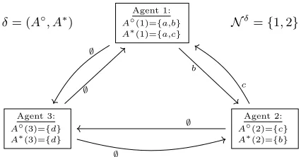
Figure 1: Scenario of Example 1 with a deal.

Section 4.3). This positive result is then tempered by two further results. First, we show that we must admit arbitrar-ily complex (yet semi-local) deals (see Section 4.4), and we must allow for the possibility of exponentially long sequences of deals before convergence is realised (see Section 4.5).

4.1

Deals and Sequences of Deals

A deal δ= (A, A0) is a pair of two (distinct) allocations A

andA0. The set of agentsinvolved in the dealδis denoted byNδ

, i.e.,Nδ

:={i∈ N |A(i)6=A0(i)}.

Example 1. Consider the set of goods G = {a, b, c, d}, the set of agents N ={1,2,3}, and the two allocations

A◦= ({a, b},{c},{d}) andA∗= ({a, c},{b},{d}). The deal

δ= (A◦, A∗) with involved agents Nδ _{= {1,2}, in which} agent 1 gives itembto agent 2 and receives itemcin return, is visualised in Figure 1.

Note that a single deal may include any number of agents and goods (even if we think of a typical deal as involving just a few of each). We would like the agents to agree on a sequence of deals that—somehow—converges to an alloca-tion that minimises inequality. Let us first exclude two ap-proaches that are definitely not useful. First, we could give the agents complete freedom what deals to negotiate. This protocol cannot ensure convergence, as we cannot exclude the possibility of loops (e.g., they may indefinitely alternate betweenA◦andA∗of Figure 1). Second, from any given al-location we could only permit a single deal, namely the deal that takes us straight to the optimal allocation. This also is not useful, as it would not leverage any of the potential power of the distributed approach and simply reduce it to a fully centralised optimisation problem.

4.2

No Convergence by Local Deals

We are looking for a criterion to select admissible deals such that (i) any sequence of admissible deals eventually leads to an optimal allocation and (ii) the agents involved in any given deal are able to determine locally whether that deal is admissible. But how should we define ‘locality’ in this context? Endriss et al. [14] call a criterion for determining the admissibility of a dealδ= (A, A0)local if and only if the question of whether δ is local can be answered by looking only at the set{(i, ui(A), ui(A0))|i∈ Nδ}. In other words, admissibility should only depend on the utility levels of the agents involved before and after the deal.

Proposition 3. It is impossible to always decide whether a given dealδ= (A, A0)would decrease inequality as defined by the Atkinson index by only inspecting the utility levels of the agents involved inδ in allocationsAandA0.

Proof. We construct an example where a given deal would decrease inequality in one scenario but increase it in another, while the local information on the utility levels of the agents involved in that deal is the same in both scenar-ios. Consider the two scenarioshN,G,U1i and hN,G,U2i,

withN ={1,2,3}andG={a, b, c, d}. The additive collec-tions of utility funccollec-tionsU1 and U2 are defined in terms of

the values the agents assign to each of the items:

U1 a b c d U2 a b c d

1: 2 1 3 4 1: 2 1 3 4

2: 2 5 2 1 2: 2 5 2 1

3: 1 2 1 6 3: 3 2 3 2

Now consider the dealδ = (A◦, A∗) between allocations

A◦= ({a, b},{c},{d}) andA∗ = ({a, c},{b},{d}), which is the same deal we had already considered in Figure 1. Let us compute the Atkinson index for each of the two allocations in each of the two scenarios:

ScenariohN,G,U1i ScenariohN,G,U2i

I(A◦) : 1− 3

√

3·2·6

1 3·(3+2+6)

≈0.099 1− 3

√

3·2·2

1 3·(3+2+2)

≈0.019

I(A∗) : 1− 3

√

5·5·6

1 3·(5+5+6)

≈0.004 1− 3

√

5·5·2

1 3·(5+5+2)

≈0.079

Thus, in the first scenario, δ decreases inequality, while in the second scenario,δincreases inequality. Nevertheless, the two agents involved inδcannot distinguish between the two scenarios. Hence, there can be no local criterion for the admissibility of deals that would allow us to always select deals that decrease inequality.

For comparison, when optimality is defined in terms of utilitarian social welfare, egalitarian social welfare, or Nash social welfare, local criteria for selecting deals that ensure a social improvement do exist [14, 23]. When the goal is to compute an envy-free allocation, there exists no suitable local criterion, but this hurdle can be overcome by slightly relaxing the requirements [10]. We shall follow a similar route.

4.3

Convergence by Semi-Local Deals

Recall that the computation of the Atkinson index involves both the geometric mean and the arithmetic mean of the utilities of all agents. On the one hand, the local information on the utility levels of the involved agents is sufficient to determine both whether (i) the geometric mean increases or decreases, and whether (ii) the arithmetic mean increases or decreases.1 On the other hand, the underlying reason for the impossibility stated in Proposition 3 is that, nevertheless, this local information is not sufficient to determine which of these two effects is stronger, and thus whether inequality will increase or decrease.

We now define asemi-local criterion for the admissibility of deals that relaxes the constraints on the information avail-able a little and thereby allows us to overcome this problem.

1

This is precisely the reason why it is possible to design local criteria for agents wishing to compute allocations with maximal Nash and utilitarian social welfare, respectively.

The central idea is to allow the agents to also access µ(A), the (arithmetic) mean of the utilities ofall agents (not just the involved agents) before the deal. Given µ(A) and the usual local information, we can compute µ(A0) for another allocationA0reached by the dealδ= (A, A0) as follows:

µ(A0) = µ(A) +1

n·

X

i∈Nδ

(ui(A0)−ui(A))

We still do not have full access to the geometric mean of all utilities, but only to the extent to which it changes during the deal. As will become clear shortly, this is not a problem. Let us call a dealδ= (A, A0) anAtkinson dealif and only if it satisfies the following condition:

n q

Q

i∈Nδui(A)

µ(A) >

n q

Q

i∈Nδui(A0)

µ(A) + 1

n· P

i∈Nδ(ui(A0)−ui(A)) Observe that we can determine whether a given deal is an Atkinson deal using semi-local information only: we require the utility levels inAandA0 for the involved agents as well as the mean value of the entire society inA. The good news is that this is sufficient to allow us to compute an optimal allocation in a distributed manner:

Theorem 4. For every scenario and initial allocation, every sequence of Atkinson deals will eventually result in an allocation that minimises inequality, as defined by the Atkin-son index.

Proof. First, observe that a deal decreases inequality if and only if it is an Atkinson deal (this is immediate from the definitions of Atkinson index and Atkinson deals).

As there are only a finite number of allocations, any se-quence without cycles has to terminate eventually. As every deal in the sequence strictly decreases inequality, there can-not be any cycles, which proves termination. Finally, it is impossible for the terminal allocation A to not have min-imal inequality, as then there would have to exist another allocationA0 with lower inequality, which would make the deal δ = (A, A0) an Atkinson deal, i.e., A could not have been terminal in the first place.

4.4

Necessity of Complex Deals

Theorem 4 shows that we will always reach an allocation with minimal inequality, provided we keep on contracting new Atkinson deals as long as any such deals exist. But our result does not say anything about how complex these deals are. Ideally, we would prefer deals that involve the exchange of only a small number of goods between a small number of agents. So we may ask whether a given deal, particularly a deal of high structural complexity, might ever becomenecessary for reaching an allocation with minimal inequality. Unfortunately, this is indeed the case:

Theorem 5. For every deal δ, there exist utility func-tions and a starting allocation, such thatδ is necessary for reaching an allocation that minimises inequality, as defined by the Atkinson index, by means of Atkinson deals only.

Theorem 5 is bad news since it shows that, if we want to reach an optimal allocation by using Atkinson deals, it might be unavoidable to use very complex deals—even involving all agents and all items. The proof is omitted for lack of space. It makes use of Lemma 7 below which covers the special case whereδ is notindependently decomposable (to be defined shortly). For the remaining cases, it uses the fact that any other deal can be decomposed into a sequence of deals each of which is not independently decomposable.

In this context, a dealδ= (A, A00) is calledindependently decomposableif it concerns two separate sets of transactions between two disjoint sets of agents, i.e., if there exists a third allocationA0 such that, for the dealsδ1= (A, A0) and

δ2= (A0, A00), it is the case thatNδ1∩ Nδ2 =∅[14].

To prove necessity of all independently decomposable deals, we require the following technical lemma.

Lemma 6. For everyn∈N>1, the function

T : [0,1] → [0,1]

x 7→ 1−

n

√

1−x

1−x n

is strictly monotonically increasing and thus bijective.

Proof. Tis well-defined and differentiable. Furthermore

T(0) = 0, T(1) = 1, and _dd_xT(x) = (n−1)x(1−x)( 1n

−1)

(n−x)2 >0 holds for allx∈]0,1[, which implies the claim.

We can now show that every deal that is not indepen-dently decomposable is necessary in the above sense:

Lemma 7. For every deal δ = (A, A0) that is not inde-pendently decomposable, there exist utility functions(ui)i∈N

and a starting allocation, such thatδis necessary for reach-ing an allocation that minimises inequality, as defined by the Atkinson index, by means of Atkinson deals only.

Proof. For the given deal δ = (A, A0), we construct a utility function for every agent. AsAand A0 are different, there is at least one agentjwithA(j)6=A0(j). We fix thisj

and let 0< x <1. We now define the utility functions for any given bundleB∈2G as

ui(B) = 

   

   

1 ifA0(i) =B,

1 if (i6=j) andA(i) =B,

1−x if (i=j) andA(i) =B,

1

i+1 otherwise.

It is now easy to see thatI(A0) = 0 and

I(A) = 1−

n

√

1−x

1−x n

.

Next, we show that for any different allocation A∗ we have I(A∗) > 0. As the deal δ is not independently de-composable, there is at least one pair of agents k, ` with

uk(A∗)6=u`(A∗): otherwise, we would haveui(A∗) = 1 for alli∈ N, meaning thatA∗agrees with eitherAorA0for ev-ery agent, i.e.,δwould be independently decomposable into the deals (A, A∗) and (A∗, A0), contradicting our assump-tions. Thus, by Lemma 1, we must have that I(A∗) >0. As there are only finitely many possible allocations, we get

min A∗6=A,A0I(A

∗ )>0.

We now choose some ε with 0< ε < minA∗6=A,A0I(A∗)

and then set xsuch thatI(A) =ε, which is possible due to Lemma 6. Hence, we have 0 =I(A0) <I(A)<I(A∗). Thus, in this scenario, from allocationA,δ= (A, A0) is the only deal reducingI, and thus the only Atkinson deal.

Our construction used in the proof of Lemma 7 is simi-lar to the construction used to derive necessity results for utilitarian and egalitarian social welfare [14] as well as Nash social welfare [23]. In those other settings, not only are all non-independently decomposable deals necessary, but these are theonly such deals. So Theorem 5 is a bad surprise, as in the present setting the situation is worse and even deals that are independently decomposable are necessary. The following example also illustrates this fact:

Example 2. Consider the (additive) scenario hN,G,U i, withN ={1,2,3,4}andG={a, b, c, d}. The collectionU

of additive utility functions is defined in terms of the values the agents assign to each of the items:

U a b c d

1: 4 10 4 4

2: 10 3 3 3

3: 2 2 2 10

4: 1 1 10 1

Now consider the deal δ = (A, A0) between allocations

A = ({a},{b},{c},{d}) and A0 = ({b},{a},{d},{c}). This deal is decomposable; there are two possible de-composition sequences, (A, Ai1_{, A}0_{) and (A, A}i2_{, A}0_{) with}

Ai1_{= ({a},{b},{d},{c}) andA}i2 _{= ({b},{a},{c},{d}).} AsUis additive, only allocations which assign exactly one item to each agent are not completely unfair. So there are only 4! allocations with inequality not equal to 1, but from these, onlyAi1_,Ai2_{, andA}0_{have a different inequality from}

A. The values ofIfor these four allocations are as follows:

I(A) : = 1− 4

√

4·3·2·1

1

4·(4+3+2+1)

≈0.115

I(Ai1_{) = 1−} 4 √

10·10·2·1

1

4·(10+10+2+1)

≈0.346

I(Ai2_{) = 1−} 4 √

4·3·10·10

1

4·(4+3+10+10)

≈0.128

I(A0) = 1− 4

√

10·10·10·10

1

4·(10+10+10+10) = 0

Finally, we are able to show that deals involving all agents and all goods can become necessary even for additive

scenarios—at least when the number of goods equals or ex-ceeds the number of agents. Again, we omit all details for lack of space.

4.5

Path Length to Convergence

In this section, we are interested in the number of deals needed to reach an optimal allocation. It is clear that, given a starting allocationA, it is always possible to reach an opti-mal allocationAoptwith at most one Atkinson deal: just use

the deal asδ= (A, Aopt)—unlessA already is optimal and

no deal is needed. It thus is more interesting to ask how long a sequence of Atkinson deals from an initial to an optimal allocation can be in the worst case. It is easy to establish an upper bound: First, observe that there arenm_possible allo-cations (recall thatn=|N |andm=|G|). Second, observe that, since every Atkinson deal strictly reduces inequality, we cannot visit any allocation twice. Hence, there can be at mostnm_{−1 deals in total. We will show that there are} scenarios for which this theoretical maximum can in fact be reached. To do so, we will construct a scenario where no two allocations produce the same inequality. We start showing this for the case of two agents in Lemma 8, before we proceed to the general case of this assertion in Lemma 11.

Lemma 8. For two agents and m goods, m ∈ N, it is possible to define utility functions such that any two distinct allocations have a different value ofI.

Proof. The proof of this lemma is inspired by the proof of Lemma 1 in the work of Ramezani and Endriss [23] for the Nash social welfare. We assign to agents 1 and 2 the prime numbers 2 and 3, respectively. Now suppose each agent has an ordering on all possible 2mbundles, andu1(B) = 2jifB

is thejth_{bundle in the first agent’s ordering. Analogously,} letu2(C) = 3j ifC is thejth bundle in the second agent’s

ordering. In an allocationA, agentireceives the (jAi) th

bun-dle in his ordering. It is easy to see that any two allocations

AandA0 have different Nash social welfare, since

swnash(A) = 2j

1

A_·3j2A_{= 2}j

1

A0 ·₃j

2

A0 _=swnash(A0₎

would imply directly jA1 = j

1

A0 and j2A = j

2

A0 due to the

unique prime factorisation of every integer.

Now we will show that alsoI(A) =I(A0) impliesA=A0:

I(A) =I(A0)

=⇒ 1−

p

swnash(A)

µ(A) = 1− p

swnash(A0)

µ(A0₎

=⇒

p 2j1

A·3jA2

1 2 ·(2

j1

A+ 3jA2)

= p

2jA10 _·3jA20

1 2·(2

j1

A0 + 3j

2

A0)

=⇒ 2jA1 _·3j2A_·(2j1A0_{+ 3}j 2

A0₎2_{= 2}j

1

A0 ·₃j

2

A0 ·₍₂j

1

A_{+ 3}j2A₎2_. As (2j_{+ 3}j0_{)≡0 mod 2 can never hold for any (j, j}0

)∈ {1, . . . ,2m}2

and also (2j+ 3j0)≡0 mod 3 can never hold for any (j, j0)∈ {1, . . . ,2m_}2_{, the unique prime factorisation}

of each side of the last equation leads again directly toj1A=

jA10 andj2_A=j2_A0 which impliesA=A0.

We will require the following technical lemma:

Lemma 9. Letn∈N>2 andj1, j2, k1, k2>0. Then

1−

n

√

2j1_·3k1

1

n(2

j1_{+ 3}k1₎ = 1− n

√

2j2_·3k2

1

n(2

j2_{+ 3}k2₎

holds iffj1=j2 andk1=k2.

Proof. This lemma can be be proved by proceeding anal-ogously to the reasoning in the proof of Lemma 8.

The proof of Lemma 8 cannot easily be generalised for more than 2 agents, as the argumentation with the modulo calculation does not hold any longer: (2i_{+ 3}j_{+ 5}k_{) mod 5} can be equal to 0 fori=j=k, e.g., (21+ 31+ 51) mod 5 = 0. Nevertheless, the closely related Lemma 9 will help us to prove the generalised statement for any number of agents. But first, we prove one further technical lemma:

Lemma 10. Real functionsga,b:R→Rgiven by

ga,b(x) =

a·x

(b+x)k

for a, b >0andk ∈Ncan be interpolated exactly by using just two points(x1, c1),(x2, c2) of the graph of the function

if we restrict the function to valuesxb/k.

Proof. Given the two equations (b+a·xx11)k = c1 and a·x2

(b+x2)k =c2, eliminating aleads to c1x2 c2x1 =

b+x2 b+x1

k . This equation can be solved via

k r

c1x2

c2x1

| {z } τ

=b+x2

b+x1

⇒ τ x2−x1

1−τ =b,

so the interpolation is unique (meaning the equation has a unique solution (a, b)).

This means that, if two functions of the above type agree on their values for two (large enough) values ofx, then they already have to be identical. We will need this property for constructing utility functions that imply different values ofI

for each possible allocation in the corresponding scenario.

Lemma 11. For any natural numbersnandm, there ex-ists a scenariohN,G,U iwith|N |=nand|G|=msuch that any two distinct allocations differ in inequality, as defined by the Atkinson index.

Proof. We consider the scenariohN,G,U iand construct utility functions that fulfil the claim. As the elements ofU

are the functionsui: 2G→R>0, it is possible to store all the

information ofU in then×2m _{matrix P = (p}

i,j)j=1,...,2 m i=1,...,n with pij =ui(Bj). Herby we suppose some arbitrary, but given ordering (B1, . . . , B2m) of the elements of 2G. For givenn, m∈N, we fill this matrix recursively to obtain the

desired result. We start the recursion with the first two rows and the following entries:

P= 

     

21 ₂2 _{. . . 2}2m

31 32 . . . 32m

∗ ∗ . . . ∗

. .

. ... . . . ...

∗ ∗ . . . ∗



     

.

of this collection of 2m+1 _{real numbers. Letp= (p(1), p(2))}

andq= (q(1), q(2)) be elements of

{21,22, . . . ,22m} × {31,32, . . . ,32m}.

Then, with the shorthand notationQ p =

Q2

i=1p(i) and

P p=

P2

i=1p(i), we see that

1− 2 q Q p 1 2 P p

= 1−

2 q Q q 1 2 P q

implies, by Lemma 9, that p = q. (This means, sloppily speaking, that similarly as in Lemma 8, if utilities are given by the already existing entries of P, any two different ‘al-locations’ exhibit a different level of inequality—they only have the same level if they are the same. At this stage, we cannot speak of real allocations andIyet, since we are only considering the utilities of bundles for a subset consisting of two agents. We therefore also cannot computeI, but a similar value by taking into account only those agents that are already involved. We make this more formal below.)

We generalise this property to bigger collections of entries of the matrixP. Let 16`6n and 16 k62m<sub>. Suppose</sub> we have already fixed values for the entries of the first`−1 rows and for the firstk−1 entries of the`th row. For every 16i6`−1, we define

Pi:={pi,j : 16j62m} ⊂R

as the set of entries in the ith row of P, corresponding to the utilities that agent i assigns to the possible bundles, and the Cartesian productP(`−1):=P1×. . .×P`−1. For

the elements p = (p(1), p(2), . . . , p(`−1)) of P(`−1)

(con-sisting of one entry from each of the already filled rows ofP), we use the shorthand notationQ

p = Q`−1

i=1p(i) and

P p=

P`−1

i=1p(i).

We call a collection of the first ((`−1)·2m_{+k−1) entries} from P feasible, if—sloppily speaking—for every choice of one entry from each already filled row, i.e., for each set of utilities for the possible bundles, any two ‘allocations’ would exhibit a different value of inequality (again, we cannot re-ally speak ofI yet, as we only consider apartialallocation as long as the matrix is not entirely filled, but this helps for the intuition). More formally, this means in the case of

k= 1 (when the first entry of each row is computed) that

1−

`−q1 Q

p

1

`−1(

P p)

= 1−

`−q1 Q

q

1

`−1(

P q)

implies p = q and i = j for any p, q ∈ P(`−1) and 16i, j62m. If k > 2, we call the collection of the (`−1)·2m_{+k−1 already fixed entries ofP feasibleif}

1−

` q

Q p·p`,i

1

`( P

p+p`,i) = 1−

` q

Q q·p`,j

1

`( P

q+p`,j)

impliesp=qandi=jfor anyp, q∈P(`−1)and 16i, j < k. The recursion step now is to fix the value forp`,ksuch that the new collection of the (`−1)·2m_{+k−1 +1then fixed} entries ofP is also feasible. Table 1 illustrates the situation of the recursion step. The entry to be fixed is marked by anx. As we have seen in the remark after Lemma 9, just taking powers of primes is not helpful. We therefore define real functions that feature the property used in Lemma 10.

Table 1: The partially filled matrix P in the recur-sion step in the proof of Lemma 11.

           

p1,1 . . . p1,2m .

.

. . .. . .. . .. . .. . .. ...

p`−1,1 . . . p`−1,k−1 p`−1,k p`−1,k+1 . . . p`−1,2m

p`,1 . . . p`,k−1 x ∗ . . . ∗

∗ . . . ∗ ∗ ∗ . . . ∗ . . . . .. . .. . .. . .. . .. ... ∗ . . . ∗ ∗ ∗ . . . ∗            

We will start with the recursion step fork= 1. We now have to fix the value forp`,1. We define the family of

func-tions (fp)p∈P(`−1) with

fp: [0,∞) → [0,1]

x 7→ 1−

` q

Q p·x

1

`( P

p+x)

.

Any pair of distinct functions of this family cannot inter-sect more than once if we restrict them to a suitable interval of the form [π1,∞[ for some π1 ∈ R (which will be

deter-mined later on). To see this, we observe the connection to Lemma 10. The equation

1−

` q

Q p·x1

1

`( P

p+x1)

= 1−

` q

Q p·x2

1

`( P

p+x2)

is equivalent to

Q p·x1 (P

p+x1)` =

Q p·x2 (P

p+x2)`

.

Letp, q∈P(`−1)be given. Ifx1 andx2 are large enough

(for example 0<P p/`,

P

q/`x1 < x2), thenfp(x1) =

fq(x1) andfp(x2) =fq(x2) implyp=q. This is true due to

Lemma 10.

Letπ1= maxp∈P(`−1)P<sub>p</sub>/`. Then if we restrict the fam-ily (fp)_p∈P(`−1) to values greater thanπ1, any pair of those

functions can intersect not more than once by the above analysis. Letπ2be the largestx-value such that two of these

functions intersect. If we choose forp`,1a value greater than

π2, we obtain that

1−

` q

Q p·p`,1 1

`( P

p+p`,1) = 1−

` q

Q q·p`,1 1

`( P

q+p`,1) impliesp=q for anyp, q∈P(`−1).

The recursion step for k > 1 is almost the same. We basically just have to replace p`,1 by p`,k. Fur-thermore, we have to choose for p`,k a value not only greater than the corresponding π2, but also greater that

some other lower bound implicitly given by the set Z =

1− ` √Q

q·p`,i 1 `(

P

q+p`,i)

q∈P(`−1)_,16i<k

.As maxZ <1, choosingx

large enough will result in 1> fp(x)> z for allp∈P(l−1) and z ∈ Z. This can be done since (i) limx→∞fp(x) = 1, and (ii) fp(0) = 1 if an only if x = 0 hold for all

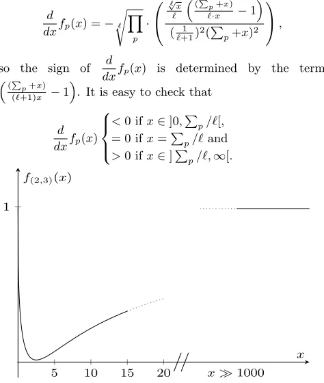
We also refer to Figure 2 for an intuition: All functions

fp have the shape of the function shown in the plot. In particular, all functions of this type are differentiable with

d

dxfp(x) =−`

s Y

p

·



 ` √

x `

(P

p+x)

`·x −1

(_`+11 )2₍P p+x)2



,

so the sign of d

dxfp(x) is determined by the term

₍P

p+x)

(`+1)x −1

. It is easy to check that

d dxfp(x)



 

 

<0 ifx∈]0,P p/`[, = 0 ifx=P

p/`and

>0 ifx∈]P p/`,∞[.

5 10 15 20

1

x1000

x f(2,3)(x)

Figure 2: A sketch of the function fp ∈(fp)_p∈P(`−1)

with `= 3 and p= (2,3). All functions used in the proof of Lemma 11 have a similar shape, in particu-lar we use thatlimx→∞fp(x) = 1for all fp.

Now let us checkP= (pi,j)j=1,...,2 m

i=1,...,n . By construction, the function F:P(n)_{→[0,1], p7→1−} n

√Q

p 1

n(

P

p)

is injective. We

defineUN,G:={u(A) :Ais an allocation inhN,G,U i}.Then

UN,G⊆P(n)andF |UN,G=I|UN,G, completing the proof.

The uniqueness property just established now is key to proving the result announced earlier (recall once more that

nis the number of agents andmis the number of goods):

Theorem 12. A sequence of Atkinson deals leading to an allocation that minimises inequality, as defined by the Atkin-son index, can consist of up tonm_{−1deals, but not more.}

Proof. There arenmpossible allocations (each of them

items may be given to any of thenagents). By Lemma 11, there exist scenarios for which each of these allocations has a unique value of I. Then, by ordering all allocations in descending order by their value of I and by defining the corresponding deals between these allocations, we obtain a sequence of nm−1 deals. Each of these deals decreases inequality and therefore is an Atkinson deal. The argument for why there can never be more thannm−1 Atkinson deals in a row has been given at the beginning of Section 4.5.

5.

CONCLUSION

We have shown that the Atkinson index, one of the most important social fairness criteria in the literature, can be

optimised in a distributed manner (Theorem 4) and thus is suitable for implementation as an objective in a multiagent system. We have been able to do so despite two inherent difficulties: the fact that the problem of finding an opti-mal allocation (with perfect equality) is NP-hard (Proposi-tion 2), and the fact that the essence of what it means to re-duce inequality cannot be captured locally (Proposition 3). While most other social criteria studied in the context of multiagent resource allocation also require us to solve com-putationally intractable optimisation problems [9], the only other such criterion that also shares the second difficulty and that nevertheless has been analysed successfully using the distributed approach is envy-freeness [10].

While Theorem 4 is encouraging, our additional results show that implementing this solution still comes with sig-nificant practical challenges. First, agents must be able to agree on arbitrarily complex exchanges of resources, without any limits on either the number of agents or the number of resources involved (Theorem 5). Second, the number of ex-changes implemented before an optimal allocation is reached can get very high and in the most extreme case we might end up visiting every logically possible allocation along the way (Theorem 12). For these negative results in particular, we have made use of analytical techniques from the basic calculus toolbox, which is unusual in the field of multiagent resource allocation and which we hope might be useful to others working on related problems.

We also hope that our work will inspire other researchers in multiagent systems, first, to use the formal notion of social inequality in the design of practical multiagent systems and, second, to further advance our state of knowledge regarding the algorithmic challenge of minimising inequality in a mul-tiagent system. Both aspects are currently underrepresented in multiagent systems research (the very few exceptions in-clude the works of Lesca and Perny [19] and Endriss [13]), even though inequality indices are widely studied and used in practice across much of the social sciences.

Our work also suggests a number of very concrete avenues for future research. First, is a similar analysis possible for other inequality indices? For the Gini index [16], we con-jecture that it would be difficult to achieve optimisation in a distributed manner without making major concessions re-garding the definition of the ‘locality’ of a deal. For the Theil index [28], another popular inequality index, our own prelim-inary results show that distributed optimisation likely will be possible, but in a less elegant manner than for the Atkinson index. Second, how obstructive are our negative results in practice? To address this question, we might generate a sce-nario (using synthetic preferences or preferences extracted from a real-world problem) and simulate what happens when agents randomly choose between one of the Atkinson deals currently available to them (possibly giving more weight to structurally simpler deals). One could investigate how often such a system gets stuck in a state where all available deals exceed some given structural complexity threshold (to assess the practical relevance of Theorem 5). One could also count the average number of deals contracted in such a system (to assess the practical relevance of Theorem 12).

6.

ACKNOWLEDGMENTS

REFERENCES

[1] P. D. Allison. Measures of inequality.American Sociological Review, 43(6):865–880, 1978.

[2] A. B. Atkinson. On the measurement of inequality.

Journal of Economic Theory, 2:244–263, 1970. [3] A. B. Atkinson.Inequality. Harvard University Press,

2015.

[4] S. Bouveret.Allocation et Partage Equitables de Ressources Indivisibles: Mod´elisation, Complexit´e et Algorithmique. PhD thesis, ISAE Toulouse, 2007. [5] S. Bouveret, Y. Chevaleyre, and N. Maudet. Fair

allocation of indivisible goods. In F. Brandt,

V. Conitzer, U. Endriss, J. Lang, and A. D. Procaccia, editors,Handbook of Computational Social Choice, chapter 12. Cambridge University Press, 2016. [6] S. Bouveret and M. Lemaˆıtre. Computing

leximin-optimal solutions in constraint networks.

Artificial Intelligence, 173(2):343–364, 2009. [7] I. Caragiannis, D. Kurokawa, H. Moulin, A. D.

Procaccia, N. Shah, and J. Wang. The unreasonable fairness of maximum nash welfare. InProceedings of the 17th ACM Conference on Economics and Computation (EC-2016), pages 305–322. ACM, 2016. [8] A.-L. Cauchy. Cours d’analyse.OEuvres Completes,

Bd, 3, 1821.

[9] Y. Chevaleyre, P. E. Dunne, U. Endriss, J. Lang, M. Lemaˆıtre, N. Maudet, J. Padget, S. Phelps, J. A. Rodr´ıguez-Aguilar, and P. Sousa. Issues in multiagent resource allocation.Informatica, 30:3–31, 2006. [10] Y. Chevaleyre, U. Endriss, and N. Maudet.

Distributed fair allocation of indivisible goods.

Artificial Intelligence, 242:1–22, 2017.

[11] H. Dalton. The measurement of the inequality of incomes.The Economic Journal, 30(119):348–361, 1920.

[12] P. E. Dunne, M. Wooldridge, and M. Laurence. The complexity of contract negotiation.Artificial Intelligence, 164(1–2):23–46, 2005.

[13] U. Endriss. Reduction of economic inequality in combinatorial domains. InProceedings of the 12th International Conference on Autonomous Agents and Multiagent Systems (AAMAS-2013), pages 175–182. IFAAMAS, 2013.

[14] U. Endriss, N. Maudet, F. Sadri, and F. Toni. Negotiating socially optimal allocations of resources.

Journal of Artificial Intelligence Research (JAIR), 25:315–348, 2006.

[15] M. R. Garey and D. S. Johnson.Computers and Intractability: A Guide to the Theory of

NP-Completeness. W. H. Freeman and Company, New York, 1979.

[16] C. Gini.Variabilit´a e Mutabilit´a. C. Cuppini, Bologna, 1912.

[17] M. N. Huhns and A. K. Malhotra. Negotiating for goods and services.IEEE Internet Computing, 3(4):97, 1999.

[18] Y. Kondor. An old-new measure of income inequality.

Econometrica, 39(6):1041–42, 1971.

[19] J. Lesca and P. Perny. LP solvable models for multiagent fair allocation problems. InProceedings of the 19th European Conference on Artificial

Intelligence (ECAI-2010), pages 393–398, 2010. [20] H. Moulin.Axioms of Cooperative Decision Making.

Cambridge University Press, 1988.

[21] J. F. Nash Jr. The bargaining problem.Econometrica, 18(2):155–162, 1950.

[22] N.-T. Nguyen, T. T. Nguyen, M. Roos, and J. Rothe. Computational complexity and approximability of social welfare optimization in multiagent resource allocation.Autonomous Agents and Multiagent Systems, 28(2):256–289, 2014.

[23] S. Ramezani and U. Endriss. Nash social welfare in multiagent resource allocation. InAgent-Mediated Electronic Commerce: Designing Trading Strategies and Mechanisms for Electronic Markets, volume 59 of

Lecture Notes in Business Information Processing, pages 117–131. Springer-Verlag, 2010.

[24] J. S. Rosenschein and G. Zlotkin.Rules of Encounter: Designing Conventions for Automated Negotiation among Computers. MIT Press, 1994.

[25] T. W. Sandholm. Contract types for satisficing task allocation: I Theoretical results. InProceedings of the 1998 AAAI Spring Symposium on Satisficing Models, 1998.

[26] T. W. Sandholm. Distributed rational decision making. In G. Weiss, editor,Multiagent Systems: A Modern Approach to Distributed Artificial Intelligence, pages 201–258. MIT Press, 1999.

[27] A. Sen.On Economic Inequality. Oxford University Press, 1973.