R E S E A R C H
Open Access
Distance to default and probability of
default: an experimental study
Amir Ahmad Dar
1,3*and Shahid Qadir
2* Correspondence:
[email protected] 1Department of Mathematics and
AS, B S Abdur Rahman Crescent Institute of Science and Technology, Chennai 600048, India
3Pulwama, India
Full list of author information is available at the end of the article
Abstract
The distance to default (DD) and the probability of default (PD) are the essential credit risks in the finance world. It provides an estimate of the likelihood that a borrower will be unable to meet its debt obligations. It is crucial to know which parameter effects more on DD and PD so that investor will prevent future risks.
Purpose:The purpose of this study is to investigate the effects of four parameters
(asset value of firmV, value of debtX, interest raterand the volatility of assetσat one period) on DD and PD.
Design/methodology/approach:The Black Scholes model is used to estimate the
DD and PD. To explore the effects of parameters, the author used Taguchi’s L27 orthogonal array, analysis of variance (ANOVA) and analysis of mean (ANOM), and the analysis will carry out using MINITAB software. The effect of parameters will be discussed with the main effect plot and the average response on a response plot showing the best outcomes.
Findings:ANOM identified the optimal combination where the DD is a maximum,
and the PD is a minimum. The percentage contribution of each input factor on DD and PD was estimated by conducting ANOVA. The above two (DD and PD) exists an inverse relationship.
Research limitations/implications:The rank or percentage contribution will vary
with change in the data set.
Keywords:Taguchi method, Probability of default, Distance to default, Black Scholes
Merton model, ANOM, ANOVA, Orthogonal arrays
Introduction
Designs of experiment (DOE) have delineated the significance of utilising cost-effective and simple to analyse design structures in multifactor examinations. Since the mid-1980s, the scan for quality inside items and procedures has prompted expanded use of such techniques. One of the powers behind this quality drive has been crafted by Genichi Taguchi, a Japanese designer. He has made utilisation of plan and investiga-tion techniques for little run multifactor experiments which have contributed altogether to the ongoing and proceeded with an accomplishment of Japanese industry. These systems, generally called Taguchi methods, have come to be connected in the Western industry with some achievement. Indeed, Taguchi techniques are frequently synonymous with the use of experimental designs in numerous associations. Taguchi strategies speak to straightforward yet novel uses of classical experimental designs.
Design of experiment utilising the Taguchi symmetrical cluster approach can finan-cially fulfil the requirements of solving problem and items structure advancement ven-tures. By applying the Taguchi’s strategy analysts, architects and researchers can diminish the time, assets and cash required for minimal exploratory examination. DOE gives the connection between the input and output variables. It utilising the Taguchi Orthogonal cluster approach requires legitimate arranging, the shrewd game plan of the examinations and investigation master of results. The Taguchi’s strategy turned into the standard technique for DOE application. It became up a standout among the best DOE for researchers and architects.
The fundamental point of the DOE is to get more and sensible data in regards to the in-put and outin-put variables. To get the more and sensible data, huge numbers of trails are required, yet the advanced hypothesis of examinations demonstrates that it is not in every case right. The greatest number of investigations, the immense will be an error and it prompted all the more exorbitant. It is smarter to assemble more and sensible data while doing fewer examinations. A standout among the best and better precedents is Taguchi’s technique. The Taguchi has built up a procedure to study the entire procedure parameters with just least adjusted trials, called orthogonal arrays. The fundamental point of DOE (Taguchi’s strategy) is to take a gander at which parameter (input) impacts more on yield.
The distance to default (DD) and the probability of default (PD) are the essential credit risks in the finance world. It provides an estimate of the likelihood that a borrower will be unable to meet its debt obligations. It is necessary to know which parameter impacts more on PD and DD so that the firm will deal with that parameter. In this paper, the BSM is used to estimate the DD and PD (Merton,1974; Dar and Anuradha,2017). The Merton model measures the DD and PD using BSM. It is important to figure out which parameter impacts more on DD and PD since credit hazard (default), estimation and the executives have turned out to be one of the basic parts in money-related financial aspects. A default (credit risk) is a hazard that neglects to pay business obligations, as delineation when Bank cannot return rule sum (Bank crumple). The term default basically implies an account holder who has not paid an obligation. In legitimate terms, it is indebtedness suggesting that a borrower cannot pay (Kaposty, Löderbusch, & Maciag2017)
The Taguchi L27 orthogonal array, analysis of mean (ANOM) and analysis of vari-ance (ANOVA) are being used to find which parameter affects more on DD and PD at one period. The following steps are necessary for DOE using Taguchi’s method:
1. Define the responsible/experimental value. The responsible variables are DD and PD in this work.
2. Selection of input/independent parameters. The DD and PD are depending on some parameters, that such parameters are called the input parameters. The input parameters in this study are asset value of firmV, value of debtX, interest rater and the volatility of assetσand time periodT.
3. Choosing the levels. If the performance variables are a linear of the input parameters, then the number of levels shall be two. However, if the response variables are not linear then one could go for three, four or higher levels. 4. Choosing the orthogonal array. This step is based on the input parameters and the
5. The result of response variables based on predictors assign to each column (to estimate the value of DD and PD based on the predictors in all combinations) 6. Conduct the experiment and analyse the data (applying ANOM and ANOVA).
Therefore, Taguchi L27 approach, ANOM and ANOVA are used in order to identify which parameter effect more on DD and PD. A firm will know which factor effects more on DD and PD so that a firm will look at that factor.
Literature review
The Taguchi’s method is used in every field such as engineering, chemistry, physics etc. in order to get more and efficient information regarding the parameters with a mini-mum number of experiments. It reduces the time, cost and resources.
Park et al. (2017) investigated the factors that effects on powder-binder (P-B) separ-ation in powder injection modelling. The factors are power size, initial powder volume, injection temperature and shear rate. The Taguchi method was used in order to identify which factor effects more on powder-binder separation in powder injection modelling. It was shown that initial powder volume fraction is a most necessary factor for P-B separation.
Celik et al. (2018) investigated the percentage contribution of parameters like thick-ness, Reynolds number, width and pitch on friction. It was measured that the percent-age contribution of thickness, Reynolds number and width on friction are 53.85%, 16.64% and 27.27% respectively and the factor pitch has a negligible effect on friction by using Taguchi method and ANOVA.
Madhavi et al. (2017) used the Taguchi’s method, S/N ratio and ANOVA in order to identify which parameter effects more or less on optimization of selected properties like hardness and surface roughness. It is shown that the material has a significant effect on above property. The cutting speed and feed rate had a moderate effect on hardness and surface roughness.
Sankar (2017) investigated which parameter (parameters are speed, depth of cut, feed and nose radius) effects more on AISI 52100 bearing steel. The Taguchi’s L27 method and ANOVA were used in order to identify that nose radius is the most significant con-trolled factor among the parameters that are mentioned above.
Apparaoa and Birru (2017) investigated which one of the parameter (pouring temperature, die temperature, filling time and injection pressure) effects more on the porosity formulation of aluminium alloy die casting. This study was based on the Taguchi’s method and ANOVA. In this study, it was shown that variations of the die casting process have a significant effect on the porosity formulation of aluminium alloy die casting.
Chan et al. (2014) used Taguchi’s L9 orthogonal array in order to estimate which fac-tor effects more on liquid yield from the catalytic pyrolysis of empty fruit bunch (EFB). It was shown that the catalyst loading has a significant effect on liquid yield from the catalytic pyrolysis of EFB. The parameters that were used in this study are catalyst load-ing, type of catalyst, nitrogen gas flow rate and catalyst loading.
Therefore, the objectives of this study are (a) to investigate which parameter im-pacts more on the response variable (PD and DD), (b) also measure the best com-bination where the value of DD is a maximum and value of PD is a minimum and (c) to check whether DD is a proxy measure for the PD.
Methodology
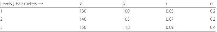
In this study, the four parameters (asset value firm, value of debt, interest rate and the volatility) are varied at three levels. The process parameters and the selected levels are presented in Table 1. And assume that the values remain fixed once they are chosen.
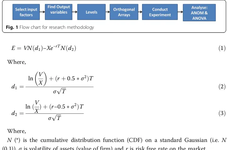
The methodology used for the research work is as per details as shown in Fig.1given below.
Distance to default and probability of default
Robert Merton (1974) developed a model by using the European call option of BSM. It is a structural model because it provides the relationship between the debt and the value of the firm. It assumes that the firm provides both equity (E) as well as debt (X), such that the value of the firm (V) is E+X. An important assumption of this model is that a firm does not pay dividends until time T (maturity). The firm will default only when the value of the firm is less than the face value of debt (X) and it will happen only at maturity period. In Merton’s model, we have two
possible scenarios:
a. If the value of firm exceeds the debt, i.e.V>X, in this case the debt holders will receiveXand the shareholders will receiveV–X.
b. If the value of debt exceeds the value of firm, i.e.V<X, in this case the debt holders will receive X and the shareholders will receive nothing.
Note:V=Xcan be collected under (b) scenario.
We can summarise the above two scenarios and the shareholders will receive
maxðVX;0Þat timeT
It implies that the values of firm’s equity at time Tcorresponds to the payoff of a European call option onV.All this makes us think about the BSM.
The famous option pricing model—the Black Scholes and Merton formula—tells us that the value of equity is equal to the European call option of BSM.
Table 1Selected process parameters and levels
Levels↓Parameters→ V X r σ
1 130 100 0.05 0.2
2 140 105 0.07 0.3
3 150 118 0.09 0.4
E¼VN d1ð Þ−Xe−rTN d2ð Þ ð1Þ
Where,
d1¼ ln V
X þ rþ0:5σ 2
ð ÞT
σpffiffiffiffiT ð2Þ
d2¼ lnðV
XÞ þ ðr−0:5σ 2Þ
T
σpffiffiffiffiT ð3Þ
Where,
N (*) is the cumulative distribution function (CDF) on a standard Gaussian (i.e. N
(0,1)),σis volatility of assets (value of firm) andris risk free rate on the market. Once the value of firmVand volatility of assetsσare known, then the distance to de-fault (DD) is calculated as follows:
d2¼ lnðV
XÞ þ ðr−0:5σ 2Þ
T
σpffiffiffiffiT ð4Þ
Under Merton’s model, a firm will default only when value of firm is less than the debt at maturity timeT.
V≤X
It can be shown that the probability V≤X, i.e.P(V≤X) is equal to
PD ¼ N −
ln V
X þ r−0:5σ 2
ð ÞT
σpffiffiffiffiT 0
B B @
1 C C
A¼1−N d1ð Þ ð5Þ
This study is based on the DD and probability of default (PD). “The PD is a credit risk which provides an estimate of the likelihood of a borrower who will be unable to meet its debt obligations”. The DD is defined as “it gives u\s idea that how much a firms value is above the threshold value”.
Fig. 1Flow chart for research methodology
Notations: “V is value of firm/asset, X is a debt value, σ is volatility of assets, T
is time period and r is the continuously compounded risk free rate” (Valverde, 2015; Wang, 2009) (Dar et al., 2019).
Experimental design (Taguchi method)
The Taguchi approach is approved in this paper in order to identify which parameter effects more on DD and PD at one period. Its aim is to find the relation between the input and the output variables/factors. The Taguchi approach is a DOE whose aim is to gather all the relevant and efficient information regarding the parameters but the Tagu-chi gather approximately all relevant with less number of experiments. The TaguTagu-chi ap-proach or Taguchi orthogonal array is a design matrix that permits the planner of experiments to test combinations of design factors that interact at various levels by car-rying out a reduced number of experiments. Dr. G. Taguchi developed this method in order to look for the relationship between the inputs and the output with the fewest number of experiments and it banishes the disadvantages of full factorial design (FFD). The FFD takes a lot of time (time consumption), cost, resources because the number of
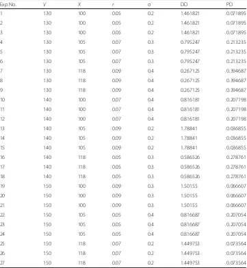
Table 2L27 (34) Standard orthogonal array (experimental design matrix with result)
Exp No. V X r σ DD PD
1 130 100 0.05 0.2 1.461821 0.071895
2 130 100 0.05 0.2 1.461821 0.071895
3 130 100 0.05 0.2 1.461821 0.071895
4 130 105 0.07 0.3 0.795247 0.213235
5 130 105 0.07 0.3 0.795247 0.213235
6 130 105 0.07 0.3 0.795247 0.213235
7 130 118 0.09 0.4 0.267125 0.394687
8 130 118 0.09 0.4 0.267125 0.394687
9 130 118 0.09 0.4 0.267125 0.394687
10 140 100 0.07 0.4 0.816181 0.207198
11 140 100 0.07 0.4 0.816181 0.207198
12 140 100 0.07 0.4 0.816181 0.207198
13 140 105 0.09 0.2 1.78841 0.036855
14 140 105 0.09 0.2 1.78841 0.036855
15 140 105 0.09 0.2 1.78841 0.036855
16 140 118 0.05 0.3 0.586526 0.278761
17 140 118 0.05 0.3 0.586526 0.278761
18 140 118 0.05 0.3 0.586526 0.278761
19 150 100 0.09 0.3 1.50155 0.066607
20 150 100 0.09 0.3 1.50155 0.066607
21 150 100 0.09 0.3 1.50155 0.066607
22 150 105 0.05 0.4 0.816687 0.207054
23 150 105 0.05 0.4 0.816687 0.207054
24 150 105 0.05 0.4 0.816687 0.207054
25 150 118 0.07 0.2 1.449753 0.073564
26 150 118 0.07 0.2 1.449753 0.073564
experiments is high. Obviously, if the number of experiments is high, cost, time and re-sources will be more (Krishnaiah & Shahabudeen,2012). The Taguchi method is a very good approach because as compared to FFD, it reduces the number of experiments, cost and resources. If we talk about the 3 levels and 4 factors, as per FFD, we need 81 experiments but as per Taguchi method, a minimum of 9 experiments are required but here the authors choose 27 trails, see Fig.2. The following standard orthogonal arrays are commonly used to DOE.
The data that are given in Table 1 are enough to calculate the values of DD and PD by using Eqs. 4 and 5. The experiment layouts for DD and PD process parameters by using Taguchi L27 approach are shown in Table2. These experiments are not randomly selected but it is based on some well-defined procedure or sampling (Unal 1991). Table2shows responses based on which factors are optimised.
Result, analysis and discussion Fitted line plot
Model Summary for DD
S R-sq R-sq (adj) R-sq (pred)
0.0776537 97.87% 97.49% 96.95%
Regression equation for DD
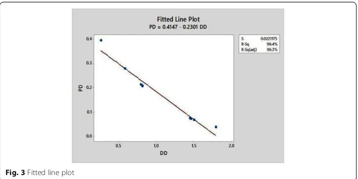
DD= 2.108 + 0.02073V−0.02749x+ 5.767r−4.667σ Fig. 3Fitted line plot
Table 3ANOM: response table for mean
Level V X r σ
1 0.8414 1.2599 0.9550 1.5667
2 1.0637 1.1334 1.0204 0.9611
3 1.2560 0.7678 1.1857 0.6333
Delta 0.4146 0.4920 0.2307 0.9333
Model summary for PD
S R-sq R-sq (adj) R-sq (pred)
0.0125575 98.99% 98.80% 98.50%
Regression Equation for PD
PD¼−0:1305−0:005543Vþ0:007432X−0:496rþ1:0444σ
The R-sq is a statistical measure which provides information how close data are to be fitted regression line. The R-sq of DD and PD is equal to 97.87% and 98.99% of the variation in the response variable. It indicates that the model provides enough fit to the data.
Note: “The normal plot of the residuals is used in order to verify the assumption that it follows the normal distribution. It was found that the residuals approximately follow straight line”(Dar and Anuradha,2018).
We can use the fitted line pot (FLP) in order to display the relationship between the DD and PD in a Minitab. In FLP, i.e. Fig.3, it is clearly shown that there is a negative relationship between DD and PD. It means when DD increase, the PD will decrease and vice versa.
The R-sq is approximately equal to 96.43%; the data fits better in the model. It indicates that the model provides enough fit to the data. The relation between DD and PD is negative which indicates that, when DD increase, the PD will decrease and vice versa as shown in Fig.3.
Analysis of mean
The mean values (ANOM) of DD and PD for each parameter at different levels were calculated by using MINITAB software. These mean values of DD and PD for each independent variable at three levels are given in Tables 3 and 4 and Figs.4 and 5 by using statistical software Minitab.
Taguchi analysis: DD versus V, X, r,σ
Look at Table 3 and Fig. 4, it clearly is shown that volatility σ affects more and the interest rate r affects less on DD. The selected numbers (italic) in Table 3 are the maximum in every column. It concludes that the best combination is V3∗X1∗r3∗σ1 because the higher DD is the best that is why the authors choose the ranking from high to low (it means that—larger the better). If you choose any combination from Table 1, you will not find a single combination where you will get maximum value of DD thanV3∗X1∗r3∗σ1.
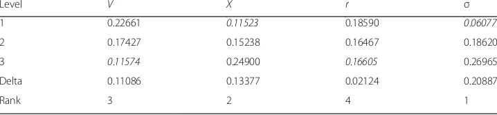
Table 4ANOM: response table for mean (PD)
Level V X r σ
1 0.22661 0.11523 0.18590 0.06077
2 0.17427 0.15238 0.16467 0.18620
3 0.11574 0.24900 0.16605 0.26965
Delta 0.11086 0.13377 0.02124 0.20887
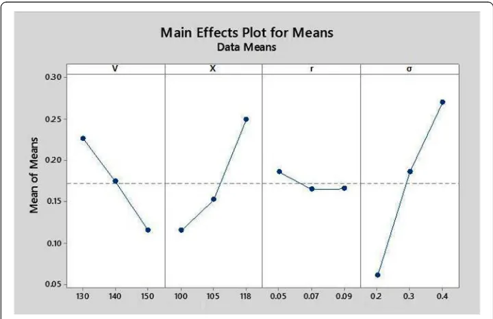
Taguchi analysis: PD versus V, X, r,σ
Look at Table 4 and Fig. 5, it clearly is shown that volatility affects more and the interest rate affects less on PD. The selected numbers (italic) in Table 4 are the minimum in every column. It is concluded that the best combination is V3∗X1∗r3 ∗σ1 (smaller the better). If you choose any combination from Table1, you will not find a single combination where you will get minimum value of PD thanV3∗X1∗r3∗σ1.
Fig. 4Main effects plot for mean (DD)
Analysis of variance
An application of ANOVA is to measure the percentage contribution of each independent variable on the dependent variable. In this study, the percentage contribution of all four parameters is measured on DD and PD as shown in Table 5. The adjusted sum of squares (Adj SS) measures how much variation for different elements of a model or term. The percentage contribution can be calculated as follows:
Percentage contribution¼ Adj SS
Total Adj SS100
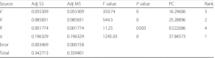
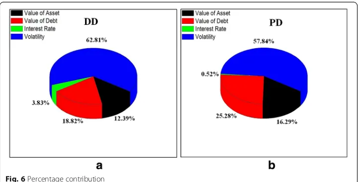
Details of the analysis of variance are shown in Table 5 and Table 6. The p value is less that 0.005 which indicates that there is difference between the treatments among the four firms. The percentage contribution of asset value of firm V, the value of debt X, interest rate rand the volatility σ on DD at one period is 12.39%, 18.82%, 3.83% and 62.81% respectively as shown in Fig. 6a, and the percentage contribution of Asset value V, the value of debt X, interest rate r and the volatility
σ on and the PD at one period is 16.29%, 25.28%, 0.52% and 57.84% respectively as shown in Fig. 6b.
Conclusion
The credit risk (PD/DD), measurement and management have become one of the essential components of financial economics. It is necessary for a firm to know which parameter effects more or less on DD and PD so that a firm will control those parameters. A famous option pricing formula (Black Scholes Mode for European Call option) was used to estimate the values of DD and PD. To measure which parameter effects more on DD and PD, the Taguchi L27 approach, ANOM and ANOVA were used. The conclusion of this study is:
Table 5Percentage contribution table for DD
Source Adj SS Adj MS Fvalue Pvalue Percentage contribution Rank
V 0.77352 0.77352 128.28 0 12.39% 3
X 1.17477 1.17477 194.82 0 18.82% 2
r 0.23947 0.23947 39.71 0 3.83% 4
σ 3.91998 3.91998 650.07 0 62.81% 1
Error 0.13266 0.00603
Total 6.2404
Table 6Percentage contribution table for PD
Source Adj SS Adj MS Fvalue Pvalue PC Rank
V 0.055309 0.055309 350.74 0 16.29606 3
X 0.085831 0.085831 544.3 0 25.28896 2
R 0.001774 0.001774 11.25 0.003 0.522686 4
σ 0.196329 0.196329 1245.03 0 57.84573 1
Error 0.003469 0.000158
a) The fitted line pot (FLP) displays the relationship between the DD and PD. It is clearly shown that there is a negative relationship between DD and PD. It means when DD increase, the PD will decrease and vice versa.
b) From ANOM, one can conclude that volatilityσaffects more and interest rater affects less on DD and PD among the four parameters at one period. The best combination among the four parameters is (V3∗X1∗r3∗σ1). This combination will provide a maximum DD and a minimum PD.
c) The ANOM measure only which parameter effects more or less on DD and PD, but the ANOVA estimates the percentage contribution of each parameter on DD and PD at one period. It was shown that volatilityσhas higest contribution and interest raterhas lowest contribution in both the models (DD and PD).
In this study, an application of Taguchi L27, ANOM and ANOVA were applied successfully. Both the statistical models (ANOM and ANOVA) displayed the same result.
Abbreviations
ANOM:Analysis of mean; ANOVA: Analysis of variance; CDF: Cumulative distribution function; DD: Distance to default; DOE: Design of experiment; FFD: Full factorial design; PD: Probability of default
Acknowledgements
We are grateful to Chief Editor Nezameddin Faghih and the reviewers for their insight comments and suggestions throughout the review process. Finally, we (Brothers) wish to thank our parents for encouraging us throughout the study. Corresponding author: the completion of this study would have been not possible if not dependent on the steadfast support and the encouragement of my wife (Samiya Jan) for her motivational speeches.
Funding Not applicable.
Availability of data and materials
The process parameters and the selected levels are presented in Table1.
Authors’contributions
Design the study: AAD. Collected the data: SQ. Analysis and interpretation of data: AAD and AQ. Drafting of manuscript: AAD. All the authors read and approved the manuscript. Special Thanks to Ikram Un Nabi Lone, Department of Physics, B S Abdur Rahman Crescent Institute of Science and Technology for his helpful suggestions for drawing the figures.
Competing interests
The authors declare that they have no competing interest
Publisher’s Note
Springer Nature remains neutral with regard to jurisdictional claims in published maps and institutional affiliations.
Author details
1Department of Mathematics and AS, B S Abdur Rahman Crescent Institute of Science and Technology, Chennai
600048, India.2Department of Commerce, Desh Bhagat University, Punjab, India.3Pulwama, India.
Received: 15 November 2018 Accepted: 5 March 2019
References
Amir Ahmad Dar, N. Anuradha, Shahid Qadir, (2019) Estimating probabilities of default of different firms and the statistical tests. Journal of Global Entrepreneurship Research 9(1).
Apparao, K. C., & Birru, A. K. (2017). Optimization of die casting process based on Taguchi approach.Materials Today: Proceedings, 4(2), 1852–1859.
Celik, N., Pusat, G. and Turgut, E., (2018). Application of Taguchi method and grey relational analysis on a turbulated heat exchanger. International Journal of Thermal Sciences 124, 85–97.
Chan, Y. H., Dang, K. V., Yusup, S., Lim, M. T., Zain, A. M., & Uemura, Y. (2014). Studies on catalytic pyrolysis of empty fruit bunch (EFB) using Taguchi’s L9 orthogonal array.Journal of the Energy Institute, 87(3), 227–234.
Dar, A. A., & Anuradha, N. (2017). Probability default in black Scholes formula: a qualitative study.J Bus Econ Dev, 2(2), 99–106. https://doi.org/10.11648/j.jbed.20170202.15.
Dar, A. A., & Anuradha, N. (2018). Use of orthogonal arrays and design of experiment via Taguchi L9 method in the probability of default.Accounting, 4(3).https://doi.org/10.5267/j.ac.2017.11.001.
Kaposty, F., Löderbusch, M., & Maciag, J. (2017).Stochastic loss given default and exposure at default in a structural model of portfolio credit risk.
Krishnaiah, K., & Shahabudeen, P. (2012).Applied design of experiments and Taguchi methods. IN: PHI Learning Pvt. Ltd. Madhavi, S. K., Sreeramulu, D., & Venkatesh, M. (2017). Evaluation of optimum turning process of process parameters using
DOE and PCA Taguchi method.Materials Today: Proceedings, 4(2), 1937–1946.
Merton, R. C. (1974). On the pricing of corporate debt: the risk structure of interest rates.The Journal of Finance, 29(2), 449–470.
Park, D. Y., Cho, H., & Park, S. J. (2017). Effects of material and processing conditions on powder-binder separation using the Taguchi method.Powder Technology, 321, 369–379.
Sankar, B. R. (2017). Analysis of forces during hard turning of AISI 52100 steel using Taguchi method.Materials Today: Proceedings, 4(2), 2114–2118.
Unal, R., & Dean, E. B. (1991).Taguchi approach to design optimization for quality and cost: an overview.
Valverde, R. (2015). An insurance model for the protection of corporations against the bankruptcy of suppliers by using the Black-Scholes-Merton model.IFAC-PapersOnLine, 48(3), 513–520.