Simplex Search-Based Brain Storm Optimization
WEI CHEN1, YINGYING CAO1, SHI CHENG 2, (Member, IEEE), YIFEI SUN3,4, QUNFENG LIU 1,5, AND YUN LI1,5, (Member, IEEE)
1School of Computer Science and Network Security, Dongguan University of Technology, Dongguan 523808, China 2School of Computer Science, Shaanxi Normal University, Xi’an 710119, China
3Key Laboratory of Modern Teaching Technology, Ministry of Education, Shaanxi Normal University, Xi’an 710062, China 4School of Physics and Information Technology, Shaanxi Normal University, Xi’an 710119, China
5Industry 4.0 Artificial Intelligence Laboratory, Dongguan University of Technology, Dongguan 523808, China Corresponding author: Qunfeng Liu ([email protected]) and Yun Li ([email protected])
This work was supported in part by the National Key R&D Program of China under Grant 2016YFD0400206, in part by the NSF of China under Grant 61773119 and Grant 61806119, and in part by the NSF of Guangdong Province under Grant 2015A030313648.
ABSTRACT Through modeling human’s brainstorming process, the brain storm optimization (BSO) algorithm has become a promising population-based evolutionary algorithm. However, BSO is pointed out that it possesses a degenerated L-curve phenomenon, i.e., it often gets near optimum quickly but needs much more cost to improve the accuracy. To overcome this question in this paper, an excellent direct search-based local solver, the Nelder–Mead Simplex method is adopted in BSO. Through combining BSO’s exploration ability and NMS’s exploitation ability together, a simplex search-based BSO (Simplex-BSO) is developed via a better balance between global exploration and local exploitation. Simplex-BSO is shown to be able to eliminate the degenerated L-curve phenomenon on unimodal functions, and alleviate significantly this phenomenon on multimodal functions. Large number of experimental results shows that Simplex-BSO is a promising algorithm for global optimization problems.
INDEX TERMSBrain storm optimization, Nelder-Mead Simplex method, global exploration, local exploita-tion, visualizing confidence intervals.
I. INTRODUCTION
Numerous scientific or engineering problems can be modeled as the following optimization problem
min f(x), s.t., x∈⊆Rn, (1)
where n is the number of controllable variables, and f(x) is the objective function. When = Rn, problem (1) is unconstrained, otherwise constrained. Specifically, whenis a rectangle or hyperrectangle, problem (1) is bound (or box) constrained.
When the objective function f(x) is nonconvex, prob-lem (1) is often hard to find the global optimumx?satisfied
f(x?)≤f(x), ∀x∈. (2)
An important reason is that there is no information which can guide tox?mathematically. Therefore, many heuristic or evo-lutionary optimization algorithms were developed for global optimization problems [8], [12], [27].
Through modeling human’s brainstorming process, the Brain Storm Optimization (BSO) algorithm proposed recently in [19] and [20] has become a promising population-based evolutionary algorithm, and has attracted more and more theoretical analysis [3], [4], [9], [11], [21], [22],
[31] and practical applications [5], [14], [17], [24], [25]. An important progress of BSO is to transform operations in the solution space to the objective space [22]. The new version of BSO is easier in implementation and lower in computational resources on the clustering strategy at each iteration. In this paper, we refer BSO to BSO in the objective space [22], unless otherwise stated.
In the BSO algorithm [22], the population evolutes through updating each individual at each iteration. Specifically, the whole population is firstly classified into two categories, the best 20% individuals are included in the elite population (elites), while the others are included in the set of regular population (normals). Then one or two parent individuals are selected randomly from either or both sets, new child indi-vidual is generated through combining these selected parent individuals linearly and then add some white noise. If the new child individual is better than the original one, the original individual will be updated with the new child individual. Such process is then repeated until stopping condition holds.
Many numerical experiments have shown that BSO is good at global exploration but not good enough at local exploitation [3], [11], [28]. Specifically, BSO can get near optimum quickly, but need much more cost to improve
accuracy. Such phenomenon is called the ‘‘degenerated L-curve’’ in this paper (Here, the L-curve of the algorithm is the so-called convergence curve of the algorithm, in order to give a visual description, we called it ‘‘L-curve’’ in this paper), and will be discussed in detail in the next section. The degenerated L-curve phenomenon prevents BSO reaching the optimum quickly with high accuracy, and therefore BSO is not suitable for optimizing directly computational expensive problems or problems needed high accuracy solutions.
The main goal of this paper is to overcome or alleviate the degenerated L-curve phenomenon of BSO. Our strategy is to combine an efficient local solver into BSO. In this way, we hope to accelerate local search firstly and then to improve the whole global search. In this paper, the Nelder-Mead Sim-plex (NMS) algorithm [16] is selected, which is one of the most well-known and efficient derivative-free optimization algorithm for local optimization [1], [26], [29]. By suitably fusing the BSO’s evolutionary search and simplex search, exploration and exploitation can be well balanced and the whole performance can be improved.
Specifically, BSO is executed for just one iteration (update the population only once), and then the best found position is regarded as a start point for NMS. Given a small budget of computational cost, NMS is executed, and the found best position is then returned back to update the best individ-ual of population. Repeat such process until some stopping condition satisfied. Since BSO is good at global exploration and NMS is good at local exploitation, our strategy can be interpreted as a repeated process including ‘‘finding a good local area’’ and ‘‘exploiting the local area’’.
The obtained algorithm, Simplex-BSO, is shown to allevi-ate significantly BSO’s degenerallevi-ated ‘‘L-curve’’ phenomenon, and perform significantly better than BSO on some popular benchmark sets by adopting the visualizing confidence inter-vals (VCI) method [13]. Although one additional parameter is employed, it is shown to be insensitive.
The remainder of this paper is organized as follows. In Section II, the BSO algorithm is reviewed briefly and its degenerated L-curve phenomenon is discussed. Then the Simplex-BSO algorithm is developed and analyzed in SectionIII. Large number of experimental results are reported in SectionIV. Finally, conclusions are drawn in SectionV.
II. BRAIN STORM OPTIMIZATION AND ITS DEGENERATED ‘‘L-CURVE’’
In this section, the BSO (Brain storm optimization in the objective space) is reviewed firstly, and then its degenerated L-curve phenomenon is discussed.
A. BRAIN STORM OPTIMIZATION IN THE OBJECTIVE SPACE
This version of BSO is proposed in [22], whose procedure is listed in Algorithm1.
In Algorithm 1, each iteration of BSO includes four components, namely ‘‘Classification’’, ‘‘Disruption’’, ‘‘New individual generation’’ and ‘‘Population updating’’.
Algorithm 1:Brain Storm Optimization (BSO)
1 Initialization: generate the initial population randomly and evaluate them;
2 whilestopping conditions do not hold do
3 Classification: classify all solutions into two categories according to their fitness values: the best 20% individuals are called ‘‘elites’’ and the others ‘‘normals’’;
4 Disruption: select an individual from the population randomly, and change its value in a randomly selected dimension;
5 New individual generation: select one or two individuals from elitists or normal to generate a child(the pseudo code of ‘‘New individual generation’’ is given in Algorithm 2);
6 Generate a new child by add a white noise to the child’s each dimension;
7 Record the new child if it is better than the current individual;
8 Update: update the whole population.
Algorithm 2:Pseudo Code of ‘‘New individual genera-tion’’
1 ifrand <pe,then 2 ifrand <pone,then
3 generate a new individual based on one randomly selected elitist;
4 else
5 generate a new individual based on two randomly selected elitists;
6 else
7 ifrand <pone,then
8 generate a new individual based on one randomly selected normal;
9 else
10 generate a new individual based on two randomly selected normals.
In ‘‘Classification’’ stage, the individuals are classified into two clusters according to their fitness values, the best 20% individuals are clustered as ‘‘elitists’’ and the remaining as ‘‘normals’’. The component ‘‘Disruption’’ is utilized to increase the population diversity, which is executed usually with a small probability and one individual’s value in one random dimension will be replaced by a random number. The ‘‘Disruption’’ strategy is often helpful for individuals to ‘jump out’ of the local optima.
new individual. Then, adding different white noises to the generated new individual in its different dimensions. The author in [22] use the following step-size function (3) to control the variances of these white noises,
ξ(t)=logsig 0.5×T−t c
×rand(t), (3)
where logsig() is a logarithmic sigmoid function,T andtare the maximum and current number of iterations, respectively, c is a coefficient to change logsig() function’s slope, and rand() return a random value between 0 and 1.
‘‘Population updating’’ is utilized to keep good solutions. The new individual generated in the above stage will be recorded if its fitness value is better than the current given individual. However, the current individual is not updated in time until all new individuals are generated and evaluated. In other words, the whole population will be updated at the end of iteration [22].
These components of the BSO algorithm [22] have been analyzed and improved for specific applications [3], [7], [23]. In this paper, we aim to improve BSO through overcoming one of its undesirable behaviors.
B. BSO’S DEGENERATED ‘‘L-CURVE’’
[image:3.576.43.271.481.680.2]It was shown that BSO is promising in solving global opti-mization problems [11], [19], [20], [30]. However, BSO is still suffering from balance of global exploration and local exploitation, just like many other global optimization algo-rithms. On one hand, global exploration provides helpful guidance and is necessary for nonconvex global optimiza-tion. On the other hand, local exploitation is very important for searching inside a potential good region and refining the solutions. But how to balance between exploration and
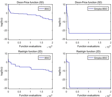
FIGURE 1. Examples of BSO’s degenerated L-curve phenomenon. BSO and Simplex-BSO are adopted to solve the Dixon-Price function and the Rastrigin function, respectively. The found best function values are plotted, and Simple-BSO’s curves are ‘‘L−type00while BSO’s are
degenerated ‘‘L−type00.
exploitation is not easy, and is often algorithm dependent and even problem dependent.
To judge BSO’s ability of balancing between exploration and exploitation, a set of 68 benchmark functions (the Hedar test set [10], will be presented detailed in Section 4) are tested, and the best function values for each function found by BSO are recorded and plotted. Two examples from the Dixon-Price function and the Rastrigin function are shown in the left subfigures of Figure1, where the right subfigures are results from our proposed algorithm Simplex-BSO.
Comparing these subfigures, it is clear that Simplex-BSO’s curves are L-type with high accuracy (about 10−25) to the global optimal value 0, which implies that Simplex-BSO find very good solutions within low computational cost (about 2000 function evaluations). However, BSO’s curves decrease slowly and finally (20000 function evaluations) reach solutions with relatively low accuracy (about 10−10). Therefore, we call it as BSO’s degenerated L-curve phe-nomenon. Among all 68 benchmark functions, there are 56 functions whose curves are similar as those in the left subfigures of Figure1. In other words, BSO’s degenerated L-curve phenomenon is popular.
Our finding implies that BSO pays less attention to local search, and has degenerated its whole performance. In next section, an efficient local solver is introduced into BSO to overcome or alleviate its degenerated L-curve phenomenon.
III. SIMPLEX SEARCH BASED BRAIN STORM OPTIMIZATION
It is shown that the BSO algorithm proposed in [22] pos-sesses a degenerated L-curve phenomenon, and it is resulted from the weakened local exploitation. In this section, an effi-cient derivative-free local solver, the Nelder-Mead Simplex method [16], is introduced into BSO. Our purpose is to overcome or at least alleviate BSO’s degenerated L-curve phenomenon through enhancing its local search.
We firstly review the NMS algorithm briefly, and then develop the Simplex-BSO algorithm.
A. NELDER-MEAD SIMPLEX ALGORITHM
The NMS algorithm was proposed by Nelder and Mead in 1965 [16], and currently it is still one of the best derivative-free (local) optimization algorithm [18].
In NMS, a simplex ofRn, which is a geometry withn+1
vertical points x1,x2, ...,xn+1, is maintained. At each
iter-ation, the worst point (with worst function value) is often replaced with a new better point, which is generated through reflection, expansion or contraction of the centroid of the best npoints around the worst one. If all these operations cannot find a better point, the worstnvertical points shrink around the best one. In this way, the simplex is always updated at each iteration, and the best vertical point will be selected as the solution when some stopping condition holds.
(outside or inside) are displayed appear in brackets after the description of the step.
Algorithm 3:Nelder-Mead Simplex (NMS)
1 Initialization: generaten+1 vertices of the initial simplex;
2 whilestopping conditions do not holddo
3 Order the points from the lowest function valuef(x1) to highestf(xn+1);
4 Computexr =2x¯−xn+1, wherex¯ =Pni=1xi/n. iff(x1)≤f(xr)<f(xn),then
5 xn+1=xr, and terminiate this iteration
(Reflection);
6 iff(xr)<f(x1),then
7 computexe= ¯x+2(¯x−xn+1),
iff(xe)<f(xr),then
8 xn+1=xe, and terminiate this iteration (Expansion);
9 else
10 xn+1=xr, and terminate this iteration (Reflection);
11 iff(xr)≥f(xn),then 12 iff(xr)<f(xn+1),then
13 computexc=(x¯+xr)/2, iff(xc)<f(xr),then
14 xn+1=xc, and terminiate this iteration
(Contract outside)
15 else
16 go to the Shrink step
17 else iff(xr)≥f(xn+1),then
18 computexcc=(¯x+xn+1)/2,
iff(xcc)<f(xn+1),then
19 xn+1=xcc, and terminiate this iteration (Contract inside).
20 else
21 go to the Shrink step
22 Shrink:xi=(xi+x1)/2, i=2, ...,n+1.
At next subsection, the NMS algorithm is introduced into BSO to improve BSO’s local exploitation ability.
B. SIMPLEX-BSO: SIMPLEX SEARCH BASED BRAIN STORM OPTIMIZATION
To overcome BSO’s degenerated L-curve phenomenon, which implies that BSO often gets near the optima quickly but needs much more cost to improve the accuracy, a nature way is to combine an efficient local solver, e.g., the NMS algorithm. The main difficulty of this strategy is how to max-imize both BSO’s exploration ability and NMS’s exploita-tion ability. After comparing several different designs, we found that the feedback between BSO’s global search
and NMS’s local search is important to improve the whole performance.
Therefore, BSO’s exploration is firstly executed, and then NMS’s exploitation is run around the found best position. Such process is repeated. Specifically, in each iteration of Simplex-BSO, an iteration of BSO is executed firstly and then the found best positionx0is used as a starting point for
NMS’s search. The NMS algorithm then begins to search the local area aroundx0, after consuming 40n(nis the dimension
of problem) computational cost, the found new best position x00 is returned back to replacex0. Repeat such process until
the stopping conditions hold. The Simplex-BSO algorithm is summarized as the Algorithm4.
Algorithm 4:Simplex-BSO
1 Initialization: generate the initial population randomly;
2 whilestopping conditions do not hold do 3 Global search: update the whole population
according to the BSO algorithm (Algorithm1). Identify the best individualx0;
4 whilesearch cost less than 40*length(x0)do
5 Local search: exploit the search area aroundx0
through executing the NMS algorithm (Algorithm3). Letx00 be the found best point;
6 Update: Update the population via replacingx0with x00.
As an integration of BSO and NMS, Simplex-BSO pro-vides a better balance between global exploration and local exploitation than BSO or NMS alone. On one hand, BSO’s global search helps to find a good starting point for NMS, which has a significant influence on the performance of the NMS method. On the other hand, NMS’s efficient local exploitation helps to find desirable solution quickly at the potential good regions.
Then we turn to consider the allocation of the whole computational cost. It is designed to be problem dependent. For each iteration of Simplex-BSO, an iteration of BSO and about 40nfunction evaluations of NMS are executed. In other words, 40nplus the size of BSO’s population is consumed at Simplex-BSO’s each iteration. Since the size of BSO’s popu-lation is often fixed, therefore, local exploitation is relatively biased asnincreases.
C. INFLUENCE OF THE ADDITIONAL PARAMETER
An additional parameter, 40n, is introduced in Simplex-BSO to balance Simplex-BSO’s global search and NMS’s local search. Although a simple rule is proposed in Algorithm4, it can be set more flexible and even adaptive.
However, our extensive experiments show that the balance parameter is insensitive for most not too hard problems. Therefore, we propose 40n in Algorithm 4for easy imple-ment. More details about the sensitivity analysis is provided in SectionIV-B.3.
IV. EXPERIMENTAL RESULTS
In this section, the Simplex-BSO is compared numerically with the following algorithms:
• NMS: an algorithm based on Nelder-Mead’s simplex
search [16];
• BSO: BSO in the objective space [22];
[image:5.576.40.269.310.728.2]Our purpose is to verify that the proposed Simplex-BSO can alleviate significantly BSO’s degenerated L-curve phe-nomenon, and to show Simplex-BSO’s good performance.
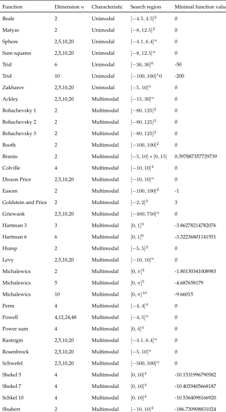
TABLE 1. Information about the Hedar test set.
Two popular sets of benchmark functions, namely the Hedar set [10] and the CEC2017 [2], are tested. Some of the hybrid and composition function of the CEC2017 set are really hard to solve, which makes the CEC2017 set harder relatively than the Hedar set.
A. THE ELIMINATION OR ALLEVIATION OF BSO’S DEGENERATED L-CURVE PHENOMENON
In this subsection, we present the numerical results on the Hedar test set [10]. Table1shows the main information of the Hedar set, including the function names, dimensions, Char-acteristic, search regions and their minimal function values. There are 16 unimodal problems and 52 multimodal problems in total.
In our experiments, 50 independent runs are executed for each problem, and all algorithms stops only when 20,000 function evaluations are consumed on the Hedar test set.
[image:5.576.300.530.363.552.2]To compare the L-curves of BSO and Simplex-BSO, 50 series of the found best function evaluations on each func-tion are averaged and plotted. Fig.2shows the L-curves on four representative functions, including 1 unimodal function (Beale) and 3 multimodal functions (Rastrigin, Griewank, Powell).
FIGURE 2. L-curves of BSO and Simplex-BSO on 1 unimodal function (Beale) and 3 multimodal functions (Rastrigin, Griewank, and Powell). Simplex-BSO eliminates BSO’s degenerated L-curve phenomenon on all 16 unimodal functions, and alleviates it significantly on 40 multimodal functions in the Hedar set.
1) L-CURVES ON 16 UNIMODAL FUNCTIONS
There are 16 unimodal functions in the Hedar set. The L-curve results on these 16 functions are very similar as that of the Beale function (see the top left subfigure in Fig.2).
are consumed. Therefore, Simplex-BSO’s L-curves are very like ‘‘L’’ while BSO’s are degenerated.
Since all L-curve results of these 16 functions are very sim-ilar, therefore we can conclude that Simplex-BSO eliminates BSO’s degenerated L-curve phenomenon on these unimodal functions.
2) L-CURVES ON 52 MULTIMODAL FUNCTIONS
There are 52 multimodal functions in the Hedar set. The L-curve results on these 52 functions show that Simplex-BSO still performs very well, and it outperforms BSO on 40 func-tions. Fig.2shows the L-curve results of the Rastrigin (2D), Griewank (10D) and Powell (24D) functions as examples.
Since 20,000 function evaluations are fixed for different dimensional functions, therefore, for low dimensional func-tions, e.g., the Rastrigin 2D at the top right subfigure, BSO often finds solutions with about 10−10accuracy slowly. The L-curve is degenerated. However, Simplex-BSO often can find better solutions with about 10−20 accuracy and with much faster convergent rate. For higher dimensional func-tions, e.g., the Griewank 10D and Powell 24D funcfunc-tions, BSO cannot find good solution since the accuracy is larger than 100. On the contrary, Simplex-BSO still can find good solutions with accuracy about 10−3for Griewank 10D and 10−10for Powell 24D.
However, there still 12 multimodal functions in the Hedar set on which Simplex-BSO is outperformed by BSO. There-fore, we can only conclude that Simplex-BSO alleviates BSO’s degenerated L-curve phenomenon on the multimodal functions.
B. DYNAMIC COMPARISON ON THE WHOLE SET
Since ‘‘L-curve’’ comparison is validation on each function, it is inconvenient and hard to obtain a comprehensive result when the number of benchmark functions is large. Therefore, in this subsection, we provide dynamic comparison results on the whole Hedar set through adopting the visualizing confidence intervals (VCI) method.
1) THE VCI METHOD
The VCI method [13] is extended from two popular bench-mark methods for deterministic optimization algorithms, namely the data profile technique [15] and the performance profile technique [6]. Through visualizing confidence inter-vals of the found best objective function values, the VCI method is shown to be convenient for benchmarking stochas-tic global optimization algorithms, especially when the set of benchmark functions or the number of algorithms is large. Hence, it is proposed to replace the traditional statistic test based methods [13].
Specifically, suppose there is a setSof optimization solvers needed to be compared numerically, and a setPof benchmark problems is selected. Then given any budget of function evaluationsµf, run each solvers∈Son each problemp∈P fornr times, and record the series of the found best function
values. After all tests finished, a 4-D matrix H with size
µf ×nr ×np×ns is obtained, where the 4-tuple element
H(k,r,j,i) denotes the found best function value duringk function evaluations at ther-th run when test thei-th solver on thej-th problem.
The matrix H is then used to generate a sample mean matrixH
H(k,j,i)= 1 nr
nr X
r=1
H(k,r,j,i) (4)
and a sample variance matrixSH2
SH2(k,j,i)= 1 nr−1
nr X
r=1
H(k,r,j,i)−H(k,j,i)2 (5)
for each algorithmi=1, ...,nson each problemj=1, ...,np
with k = 1, ..., µf function evaluations. The confidence
upper bound matrixHupper and the confidence lower bound
matrixHlowerare then defined as follows
Hupper(k,j,i)=H(k,j,i)+
2SH(k,j,i)
√ nr ,
(6)
Hlower(k,j,i)=H(k,j,i)−
2SH(k,j,i)
√ nr .
(7)
In the VCI method, H,Hupper and Hlower are analyzed
statistically with the data profile technique. The data profile is a cumulative distribution function defined for any solver s∈Sas follows
ds(κ)=
1 |P|size
p∈P: tp,s Dp+1
≤κ
, (8)
where|P| denotes the number of test problems, Dp is the
dimension of the problemp, and size{} returns the size of a set. In (8),tp,sis the number of function evaluations needed
for solver sto find a position x such that the convergence condition
f(x0)−f(x)≥(1−τ)(f(x0)−fL) (9)
holds, where x0 is the starting point, fL is the smallest
objective function value obtained by any solver within µf
of function evaluations, andτ > 0 (in this paper, we use τ =1×10⁻⁷) is a tolerance.tp.s = ∞if the condition (9)
does not satisfy afterµf function evaluations.
Roughly speaking, the VCI method adopts the data pro-file technique twice to benchmark stochastic optimization algorithms. Specifically, the data profile technique is used to analyzeHfirstly. From the generated data profiles, a winner solver can be determined in the sense of best average perfor-mance. Then the data profile technique is used to compare the winner solver’sHupper and the other solvers’Hlower. The
purpose is to confirm that the winner solver performs the best in the sense of the worst deviation.
2) DYNAMIC COMPARISONS WITH THE VCI METHOD
The VCI method allows us to compare both stochastic and deterministic optimization algorithms, and therefore is suit-able for comparison between BSOs and NMS. Two steps are needed. Firstly, we compare the average behaviors of BSO, Simplex-BSO and NMS to determine a winner algorithm. Secondly, the winner’sHupper is compared with the others’
Hlower to confirm whether the winner still performs the best
[image:7.576.48.269.223.426.2]at the worst case. If so, then the conclusion is significant statistically that the winner performs better than the other algorithms. Otherwise, the conclusion is that the winner per-forms averagely better than the other algorithms.
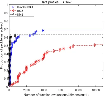
FIGURE 3. Data profiles resulted from comparing the average behaviors of BSO, Simplex-BSO and NMS on the Hedar test set. The results show that Simplex-BSO performs very well since it possesses both NMS’s good local search ability and BSO’s global search ability.
Fig. 3 shows the results of the comparison of average behaviors, where the horizontal axis is the computational cost and the vertical axis shows the proportion of problems solved. Therefore, the more close to the left top corner, the better the curve (i.e., the algorithm) is.
We can see from Fig.3that the NMS algorithm performs much better than BSO when the computational cost is small, and it can solve more than 60% problems very quickly. However, NMS cannot perform better when the computa-tional cost is larger than about 2000. On the other hand, BSO performs better and better as the computational cost increases, and finally can solve about 52% problems. This observation confirms that NMS is an efficient local optimiza-tion algorithm while BSO is a global optimizaoptimiza-tion algorithm, and moreover, the original BSO performs much worse than NMS.
From Fig.3we can see that Simplex-BSO possesses both NMS’s local search ability and BSO’s global search abil-ity. When the computational cost is less than about 2000, Simplex-BSO performs worse slightly than NMS. However, Simplex-BSO performs better and better as the computational
cost increases. Finally, Simplex-BSO can solve about 69% problems, i.e. Simplex-BSO can not solve about 21 problem (They areAckleyof dimmension 10 and 20,Hump,Levyof dimmension 10 and 20,Michof dimmension 5 and 10,Rast of dimmension 5, 10 and 20,Rosenof dimmension 5, 10 and 20,Schwof dimmension 2, 5, 10 and 20,Shekel5,Shekel7, Shekel10, Trid of dimmension 10 respectively), about 6% higher than NMS and 17% higher than BSO.
TheHupper of Simplex-BSO is then compared withHlower
of BSO and NMS. The result shows that Simplex-BSO’s worst case is outperformed by the best cases of BSO and NMS. According to the VCI method, the conclusion is that Simplex-BSO performs better averagely than both BSO and NMS.
Combined with the results in SectionIV-A, the proposed Simplex-BSO is a promising global optimization algorithm. Through adopting simplex search in BSO, the local search ability is enhanced significantly and the whole global search ability is then strengthened. However, an additional parame-ter 40nis adopted in Simplex-BSO to balance the local search and global search. The sensitivity of the parameter is analyzed in next subsection.
3) SENSITIVITY ANALYSIS OF THE ADDITIONAL PARAMETER
We adopt five different parameter values in Algorithm4 to analyze the additional parameter’s sensitivity. Specifically, 20n,30n,40n,50n,60nare adopted and tested on the Hedar set. The average behaviors of 50 independent runs are com-pared with the VCI method, and Fig.4shows the results.
FIGURE 4. Data profiles when comparing different version of Simplex-BSO with different parameter values. The results imply that this parameter is insensitive within a large period (40n,60n).
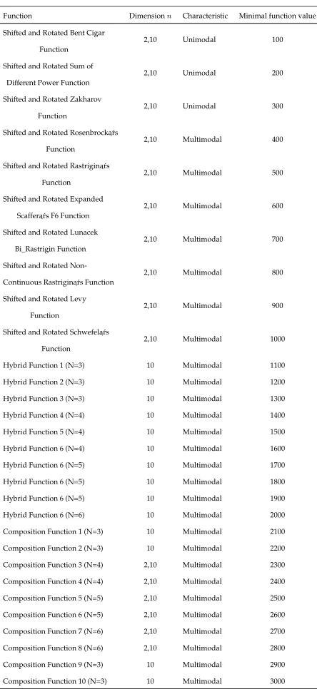
[image:7.576.303.529.426.626.2]TABLE 2. Information about the CEC’17 test suite.
two reasons why we select the smallest value in this inter-val. Firstly, all values within (40n,50n) perform very well. Secondly, a small parameter value is helpful in maintaining population diversity, and therefore enhancing good global search ability.
C. EXTENDED COMPARISON ON THE CEC2017 TEST SET
In previous subsection, Simplex-BSO has shown to be able to eliminate BSO’s degenerated L-curve phenomenon on uni-modal functions and alleviate significantly it on multiuni-modal functions in the Hedar set. Although an additional parameter is introduced, our sensitivity analysis shows that it is insensi-tive within an large interval.
In this subsection, Simplex-BSO is compared with BSO and NMS on the CEC2017 test set [2], which includes 30 dif-ferent functions and most of them are harder than those in the Hedar set. Our purpose is to verify whether Simplex-BSO still performs well.
Totally, 46 benchmark functions are tested, including all the 16 two-dimensional and 30 ten-dimensional functions in CEC2017 set. Main information about these functions are listed in Table 2. For each function, 50 independent runs are executed, and the algorithms stop only when 10,000n function evaluations are consumed, wherenis the dimension. The VCI method is adopted to analyze the test data.
1) RESULTS ON THE 2D FUNCTIONS
Fig.5shows the comparison results on 16 two-dimensional functions in CEC2017. 50 independent runs are averaged, and data profiles are generated through the VCI method.
FIGURE 5. Data profile results when comparing Simplex-BSO, BSO and NMS on 16 two-dimensional functions in the CEC2017 set.
From Fig. 5 we can see that NMS finds 3 (=16*19%) functions’ optimum very quickly but never gets better. The reason is that NMS is a local solver and often stagnates in a local optimal position. However, both BSO and Simplex-BSO can solve more and more functions as computational cost increases. Finally, Simplex-BSO solves 11 (=16*69%) functions and BSO solves 10 (=16*63%) functions, much larger than NMS’s 3 functions.
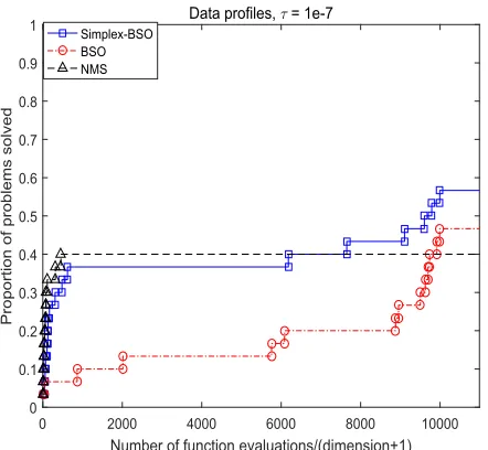
[image:8.576.305.529.293.497.2]FIGURE 6. Data profile results when comparing Simplex-BSO, BSO and NMS on 30 ten-dimensional functions in the CEC2017 set.
2) RESULTS ON THE 10D FUNCTIONS
Fig.6 shows the comparison results on 30 ten-dimensional functions in CEC2017. 50 independent runs averaged, and data profiles are generated through the VCI method.
From Fig. 6 we can see that NMS solve about 12 (=30*40%) functions and Simplex-BSO solves 11 (=30*37%) functions with the best efficiency. On the con-trary, BSO only solves 2 functions with the best efficiency.
As the computational cost increases, NMS never solves more functions, while both Simplex-BSO and BSO solves more and more functions. For instance, when the compu-tational cost increases to about 6200, Simplex-BSO solves 12 functions and BSO solves 6 functions. Finally, Simplex-BSO solves 17 (=30*57%) functions and BSO solves 14 (=30*47%) functions. Once again, Simplex-BSO performs almost always better than BSO for any given computational cost.
Averagely, Simplex-BSO still performs very well on the CEC 2017 test set. Combined with the results on the Hedar set, Simplex-BSO is a promising global optimization algo-rithm. Through adopting an efficient NMS local solver in BSO, the obtained algorithm Simplex-BSO enhances its local search significantly and improves its whole performance.
V. CONCLUSIONS
In this paper, the BSO algorithm is shown to possess the degenerated L-curve phenomenon. To overcome this prob-lem, an efficient derivative-free local solver, the Nelder-Mead Simplex method, is adopted into the BSO algorithm. The obtained algorithm, Simplex-BSO, is shown to be able to eliminate BSO’s degenerated L-curve phenomenon on uni-modal functions and alleviate this phenomenon significantly on multimodal functions. Although an additional balance parameter is introduced in Simplex-BSO, it is shown to be
insensitive within a large interval. Extensive experimental results show that the proposed Simplex-BSO algorithm is a promising global optimization algorithm.
REFERENCES
[1] M. A. Ahandani, M.-T. Vakil-Baghmisheh, and M. Talebi, ‘‘Hybridizing local search algorithms for global optimization,’’Comput. Optim. Appl., vol. 59, no. 3, pp. 725–748, 2014.
[2] N. H. Awad, M. Z. Ali, J. J. Liang, B. Y. Qu, and P. N. Suganthan, ‘‘Problem definitions and evaluation criteria for the CEC 2017 special session and competition on single objective bound constrained real-parameter numer-ical optimization,’’ School Elect. Electron. Eng., Nanyang Technol. Univ., Singapore, Tech. Rep., 2016.
[3] Y. Y. Caoet al., ‘‘A simple brain storm optimization algorithm via visualiz-ing confidence intervals,’’ inProc. 11th Int. Conf. Simulated Evol. Learn. (SEAL), 2017, pp. 27–38.
[4] S. Cheng, Q. Qin, J. Chen, and Y. Shi, ‘‘Brain storm optimization algo-rithm: A review,’’Artif. Intell. Rev., vol. 46, no. 4, pp. 445–458, 2016. [5] H. Duan, S. Li, and Y. Shi, ‘‘Predator–prey brain storm optimization for
dc brushless motor,’’IEEE Trans. Magn., vol. 49, no. 10, pp. 5336–5340, Oct. 2013.
[6] E. D. Dolan and J. J. Moré, ‘‘Benchmarking optimization software with performance profiles,’’Math. Program., vol. 91, no. 2, pp. 201–213, 2002. [7] M. El-Abd, ‘‘Global-best brain storm optimization algorithm,’’Swarm
Evol. Comput., vol. 37, pp. 27–44, Dec. 2017.
[8] C. A. Floudas and C. E. Gounaris, ‘‘A review of recent advances in global optimization,’’J. Global Optim., vol. 45, no. 1, pp. 3–38, 2009. [9] X. Guo, Y. Wu, and L. Xie, ‘‘Modified brain storm optimization
algo-rithm for multimodal optimization,’’ inAdvances in Swarm Intelligence (Lecture Notes in Computer Science), vol. 8795, Y. Tan, Y. Shi, and C. A. C. Coello, Eds. New York, NY, USA: Springer, 2014, pp. 340–351. [10] A.-R. Hedar. Global Optimization Test Problems. Accessed: Nov. 27, 2018. [Online]. Available: http://www-optima.amp.i.kyoto-u.ac.jp/member/student/hedar/Hedar_files/TestGO.htm
[11] Z. Jia, H. Duan, and Y. Shi ‘‘Hybrid brain storm optimisation and simulated annealing algorithm for continuous optimisation problems,’’Int. J. Bio-Inspired Comput., vol. 8, no. 2, pp. 109–121, 2016.
[12] Q. Liu, ‘‘Linear scaling and the DIRECT algorithm,’’J. Global Optim., vol. 56, no. 3, pp. 1233–1245, 2013.
[13] Q. Liuet al., ‘‘Benchmarking stochastic algorithms for global optimiza-tion problems by visualizing confidence intervals,’’IEEE Trans. Cybern., vol. 47, no. 9, pp. 2924–2937, Sep. 2017.
[14] X. Ma, Y. Jin, and Q. Dong, ‘‘A generalized dynamic fuzzy neural network based on singular spectrum analysis optimized by brain storm optimiza-tion for short-term wind speed forecasting,’’Appl. Soft Comput., vol. 54, pp. 296–312, May 2017.
[15] J. J. Moré and S. M. Wild, ‘‘Benchmarking derivative-free optimization algorithms,’’SIAM J. Optim., vol. 20, no. 1, pp. 172–191, 2009. [16] J. A. Nelder and R. Mead, ‘‘A simplex method for function minimization,’’
Comput. J., vol. 7, no. 4, pp. 308–313, 1965.
[17] H. Qiu and H. Duan, ‘‘Receding horizon control for multiple UAV forma-tion flight based on modified brain storm optimizaforma-tion,’’Nonlinear Dyn., vol. 78, no. 3, pp. 1973–1988, 2014.
[18] L. Rios and N. Sahinidis, ‘‘Derivative-free optimization: A review of algo-rithms and comparison of software implementations,’’J. Global Optim., vol. 56, no. 3, pp. 1247–1293, 2013.
[19] Y. Shi, ‘‘Brain storm optimization algorithm,’’ inAdvances in Swarm Intelligence(Lecture Notes in Computer Science), vol. 6728, Y. Tan, Y. Shi, Y. Chai, G. Wang, Eds., Springer Berlin Heidelberg, 2011, pp. 303–309.
[20] Y. Shi, ‘‘An optimization algorithm based on brainstorming process,’’Int. J. Swarm Intell. Res., vol. 2, no. 4, pp. 35–62, 2011.
[21] Y. Shi, ‘‘Developmental swarm intelligence: Developmental learning per-spective of swarm intelligence algorithms,’’Int. J. Swarm Intell. Res., vol. 5, no. 1, pp. 36–54, 2014.
[22] Y. Shi, ‘‘Brain storm optimization algorithm in objective space,’’ inProc. IEEE Congr. Evol. Comput. (CEC), May 2015, pp. 1227–1234. [23] Z. Song, J. Peng, C. Li, and P. X. Liu, ‘‘A simple brain storm optimization
[24] D. Verma and S. Dubey, ‘‘Fuzzy brain storm optimization and adaptive thresholding for multimodal vein-based recognition system,’’Int. J. Pattern Recognit. Artif. Intell., vol. 31, no. 05, 2017, Art. no. 1756007. [25] J. Wang, R. Hou, C. Wang, and L. Shen, ‘‘ImprovedV-Support vector
regression model based on variable selection and brain storm optimization for stock price forecasting,’’Appl. Soft Comput., vol. 49, pp. 164–178, Dec. 2016.
[26] L. Wang, Y. Xu, and L. Li, ‘‘Parameter identification of chaotic systems by hybrid Nelder–Mead simplex search and differential evolution algorithm,’’ Expert Syst. Appl., vol. 38, no. 4, pp. 3238–3245, 2011.
[27] T. Weise, Global Optimization Algorithms—Theory and Application, 3rd ed. 2011 [Online]. Available: http://www.it-weise.de/projects/book.pdf [28] Y. Yang, Y. Shi, and S. Xia, ‘‘Advanced discussion mechanism-based brain storm optimization algorithm,’’ Soft Comput., vol. 19, no. 10, pp. 2997–3007, 2015.
[29] E. Zahara and Y.-T. Kao, ‘‘Hybrid Nelder–Mead simplex search and par-ticle swarm optimization for constrained engineering design problems,’’ Expert Syst. Appl., vol. 36, no. 2, pp. 3880–3886, 2009.
[30] Z.-H. Zhan, J. Zhang, Y.-H. Shi, and H.-L. Liu, ‘‘A modified brain storm optimization,’’ inProc. IEEE Congr. Evol. Comput. (CEC), Jun. 2012, pp. 1–8.
[31] Z.-H. Zhan, W.-N. Chen, Y. Lin, Y.-J. Gong, Y.-L. Li, and J. Zhang, ‘‘Parameter investigation in brain storm optimization,’’ inProc. IEEE Symp. Swarm Intell. (SIS), Apr. 2013, pp. 103–110.
WEI CHEN received the bachelor’s and M.S. degrees from Henan University in 2006 and the Ph.D. degree from the South China University of Technology, China, in 2009 and 2014, respec-tively. From 2014 to 2016, he was engaged in post-doctoral research in control science and engi-neering with the South China University of Tech-nology. He is currently an Assistant Research Fellow with the School of Computer Science and Network Security, Dongguan University of Tech-nology. His current research interests include global optimization, evo-lutionary computation, quantum computation, and quantum evoevo-lutionary computation.
YINGYING CAO received the bachelor’s and Ph.D. degrees from the School of Mathematics and Computing Science, Sun Yat-sen University, in 2007 and 2012, respectively. From 2011 to 2012, she was a Post-Graduate Visiting Researcher at the City University of Hongkong. She is cur-rently a Lecturer with the School of Computer Science and Network Security, Dongguan Univer-sity of Technology. Her current research interests include computational intelligence, optimization algorithms, and their applications.
SHI CHENG (M’14) received the bachelor’s degree in mechanical and electrical engineer-ing from Xiamen University, Xiamen, in 2005, the master’s degree in software engineering from Beihang University, Beijing, China, in 2008, and the Ph.D. degree in electrical engineering and elec-tronics from the University of Liverpool, Liver-pool, U.K., in 2013. He is currently a Lecturer with the School of Computer Science, Shaanxi Normal University, China. His current research interests include swarm intelligence, multiobjective optimization, and data mining techniques and their applications.
YIFEI SUN received the bachelor’s and Ph.D. degrees from Xidian University, China, in 2005 and 2014, respectively. She is currently a Lec-turer with the School of Physics and Informa-tion Technology, Shaanxi Normal University. Her current research interests include artificial intel-ligence, global optimization, and evolutionary computation.
QUNFENG LIUreceived the bachelor’s and M.S. degrees from the Huazhong University of Science and Technology in 1999 and 2002, respectively, and the Ph.D. degree from Hunan University, China, in 2011. He is currently an Associate Professor with the School of Computer Science and Network Security, Dongguan University of Technology, China. His current research interests include global optimization, evolutionary compu-tation, and machine learning.