Three dimensional tidal turbine array simulations using OpenFOAM with dynamic mesh

1

Three dimensional tidal turbine array simulations using

OpenFOAM with dynamic mesh

Martin Nuernberg, Longbin Tao*

3

School of Marine Science and Technology, Newcastle University, Newcastle upon Tyne, 4

NE1 7RU, UK 5

Abstract

The flow field characteristics in the wake of an isolated tidal turbine and tidal turbine arrays 7

of up to four devices is investigated by numerical simulations solving the Reynolds Averaged 8

Navier Stokes (RANS) equation in the Open Source OpenFOAM CFD solver to make use of 9

the significantly increased availability of computational resources and multi-core processing. 10

Transient simulations utilizing the k – ω SST turbulence closure model were used in 11

combination with a dynamic mesh interface to account for the rotation of the three bladed 12

tidal turbine at constant tip speed ratio, the applicability of dynamic mesh simulations for the 13

investigation of array wakes has been shown. The velocity and turbulence characteristics are 14

compared to experiments previously conducted with a number of small scale tidal turbine 15

devices arranged in staggered array formations and tested within a low ambient turbulence 16

circulating water channel. Results showed good agreement between simulations and 17

experiments and further insight to the flow field within an array is provided, however further 18

improvements to predict the wake characteristics in array are required. 19

Keywords RANS, Arbitrary Mesh Interface (AMI), Tidal Turbine Arrays, Wake Characteristics 20

2

1.

Introduction

1

The UK has been in the leading position for design and construction of tidal turbines for a 2

number of years, as part of the continuing efforts to increase the share of renewable energy 3

sources and reducing the dependency on fossil fuels as primary means of energy supply. 4

Electricity generation from tidal stream turbines is estimated to account for about 20% of the 5

UK’s electricity demand in the future and has seen the first commercial electrical power 6

generated and supplied to a national grid in 2008. Following the successful development and 7

testing of tidal turbine prototypes and scaled demonstrator projects at dedicated test sites and 8

commercial project location (Atlantis Resources Ltd, 2016a; EMEC, 2017) the tidal stream 9

energy industry is currently seeing first array installations in open waters with construction 10

having started in autumn of 2016 (Atlantis Resources Ltd, 2016b). 11

Tidal turbine arrays are a vital step towards increasing the nation’s share of renewable energy 12

sources for the large scale generation of electricity and play a significant part in economically 13

commercialising this technology. Investigating the complex flow within tidal turbine arrays 14

plays an important role in this development as the operating environment is dominated by 15

complex flow features and geophysical characteristics which affect the performance as well 16

as lifetime reliability of devices installed in the sea. 17

Computational Fluid Dynamics (CFD) to model the hydrodynamic interactions between 18

multiple tidal turbine devices, alongside smaller scale experimental investigations will aid in 19

reducing the costs and uncertainty of developing and deploying large scale tidal turbine 20

arrays in the near future while providing useful and detailed insights into the resulting flow 21

field and optimisation of array configurations in densely spaced arrangements of tidal stream 22

3 Tidal turbine devices have been tested extensively over the last decade using experimental, 1

numerical and prototype studies for the optimisation of power production through design of 2

devices and device components such as blade sections, support structure and control systems. 3

Initial numerical assessment of tidal turbine performance and wake characteristics by 4

Harrison et al. (2010) and Turnock et al. (2011) focused on simplified turbine representation 5

in the form of actuator disks (AD), solving the Reynolds Averaged Navier-Stokes (RANS) 6

equation in combination with source terms derived from blade element momentum theory 7

(BEMT) to account for the body forces, rotation and turbulence induced by the tidal turbine. 8

Harrison et al. (2010) state that the k – ω SST turbulence closure model simulates the flow 9

conditions in the wake downstream of an actuator disk better than the k - ε model due to its 10

improved performance in adverse pressure gradients and the blending of both k – ω and k – ε 11

models. It is argued by Batten et al. (2013) that k- ω SST under predicts the rate of wake 12

recovery thus the k – ε model is used in combination with turbulence source terms on the 13

disk. These methods were found to demonstrate good agreement with experiments for the far 14

wake velocity (x/D >7) and turbulence prediction downstream of tidal turbines. Advantages 15

are improved efficiency of numerical calculations however these come at the cost of 16

introducing corrections to account for the finite number of blades and the turbine hub to 17

account for the blade induced rotation and vortices of and in the wake. 18

To further investigate wake characteristics of single turbines and small arrays, especially 19

initial wake development in the near wake of tidal turbines, more detailed representations of 20

tidal turbine rotors have been computed (RANS) by Bai et al. (2015) with k – ω SST 21

turbulence closure model and using actuator surfaces to account for the blade length and 22

chord distributions along the radial direction and showed much improved agreement over 23

previous tests with BEMT in combination with actuator disks by Bai et al. (2013) in terms of 24

4 al. (2007). Further improvements are to include other factors such as the turbine support 1

structure which along with blade design significantly affects the near wake characteristics. 2

By fully resolving the blade details of tidal turbines, the computational resources required 3

increase significantly due to the fine resolution required to accurately model the flow over the 4

turbine blades, however it no longer required using BEMT or CFD calculations to determine 5

blade performance characteristics prior to applying on actuator disks or surfaces. 6

O'Doherty et al. (2009) used fully resolved quasi-static 3D RANS calculations with a moving 7

reference Frame (MRF) validated against model tests to investigate and optimize power and 8

thrust predictions and the use of various turbulence closure models where Reynolds Stress 9

Model (RSM) was found to agree best with results. This was extended by investigating 10

dimensional scaling of performance characteristics by conducting a range of simulations with 11

increasing diameters and velocities (Mason-Jones et al., 2012) followed by a sheared velocity 12

profile and support structure by Mason-Jones et al. (2013) showing both, increased wake 13

asymmetry and cyclic loading over the blade rotation. 14

McNaughton et al. (2014) and Afgan et al. (2013) showed performance indicators for a three 15

bladed tidal turbine including support structure and also highlighted the flow field within the 16

wake. RANS and large eddy simulations (LES) are used and found performance prediction to 17

be in good agreement for most models at optimum turbine Tip Speed Ratio (TSR). The 18

combination of RANS and k-ω SST turbulence model resulted in comparable performance 19

characteristics at significantly lower computational resource requirement than LES, matching 20

the LES results for the optimum design condition. The k-ε turbulence closure model 21

performed noticeably worse in off-design conditions. Wake characteristics are shown but 22

5 A comparison between modelling tidal turbines using the approaches (AD, MRF and Sliding 1

mesh) described above is shown by Liu et al. (2016) and argues that the most realistic wake 2

representation is achieved by fully resolving the turbine geometry and there is still limited 3

information about comparison of simplified, resolved and experimental investigations of tidal 4

turbine wakes. The study showed that sliding mesh technique presents the wake 5

characteristics most accurately in the near and far wake and captures realistic transient 6

behaviour in the wake and comparison of normalized mean velocity to experiments 7

conducted by Mycek et al. (2013) showed close agreement. 8

Vennell et al. (2015) highlighted some of “key” array effects on macro and micro array level 9

design, such as the influence of array sections on the ambient and large scale flow and 10

available power characteristics. On a micro design level, the turbulence generated from 11

devices and the wake mixing and velocity recovery of a small number of turbines in close 12

proximity has a significant impact on the device spacing within the array as well as the 13

optimised design of support structures to maximise power output and reduce risk of operating 14

tidal turbines in these complex and challenging environments. 15

The far field influence of large scale electricity generation from tidal flows has been 16

investigated using simplified hydro-environmental modelling, applying one and two-17

dimensional shallow water equations and including energy extraction by a resistance 18

coefficient and as momentum sinks. The techniques have been applied for numerical 19

optimisation of array lay-outs by Funke et al. (2014) and for some proposed locations of tidal 20

energy extraction (Ahmadian and Falconer, 2012) and the environmental impact on tidal 21

basins and channels. However, these methods are not suitable to investigate the wake within 22

and downstream of tidal turbine arrays and focus on the dominant flow processes occurring in 23

6 To reduce the computational resources required to investigate the performance of multiple 1

tidal turbines operating in small arrays, actuator fences (Daly et al., 2013) and multiple 2

circular disks (Nishino and Willden (2013); Turnock et al. (2011)) have been used to speed 3

up numerical calculations and investigate the effects of energy extraction for cross stream 4

arrays that block a large proportion of the available tidal channel. It was shown that analytical 5

model and 3D RANS calculation with actuator fence revealed interactions between beneficial 6

flow effects and increased flow reduction due to increasing devices which in turn led to an 7

increased optimum blockage of the tested configurations. Numerical simulations of tidal 8

arrays have been conducted using steady state solutions with MRF to simulate the rotating 9

blades by Lee et al. (2010) investigating the distance between 6 tidal turbines arranged in a 10

generic sea side and lake environment. Optimum spacing of turbines was found to be three 11

turbine diameters and wake asymmetry due to turbine rotation could be observed. 12

Using LES study in combination with actuator lines to represent the rotation of turbine 13

blades, Churchfield et al. (2013) investigated the structure of resulting unsteady wakes and 14

determined staggered arrays to have higher efficiencies. Additionally rotating downstream 15

rows of turbines in opposite direction was found to show small benefits. The importance of 16

including tangential forces in simplified representations of tidal turbine in simulations was 17

highlighted by the existence of asymmetric wake structures. 18

A fully resolved numerical simulation with two tidal turbines arranged in line has been 19

presented by Liu et al. (2016) with a second turbine being located 8D downstream of the first. 20

The velocity contours show the downstream turbine operating with within a significantly 21

slowed down wake, most pronounced at the centre-line, and very slow moving fluid in the 22

wake of the downstream turbine. The countours also highlight areas of significantly increased 23

turbulence intensity about 4D downstream of the second turbine due to accumulation of 24

7 Due to the high costs and complex measurement arrangements for detailed flow

1

representation, few experimental array studies have been conducted, ranging from turbine 2

interactions of a small number of devices being arranged at varying longitudinal distances 3

(Mycek et al., 2014b) and small lateral offsets (Javaherchi et al., 2013) to experimental array 4

configurations (Stallard et al., 2015) with a maximum distance from first to last row of 5

turbines of 10D. Comparisons between RANS - BEMT and experimental measurements of 6

thrust and wake velocities are reported by Olczak et al. (2016) showing that inclusion of 7

device generated turbulence improved agreement between experiments and numerical 8

simulations especially in the near wake region where x/D < 4. It was also found that the 9

velocity deficit between adjacent wakes is under predicted for x/D < 8. The variations in 10

prediction of thrust coefficients on the actuator disks compared to experiments show less than 11

10% for front row, 20% for seconds and 38% for the third row, variations are increased 12

especially on the centre turbines operating in the wake of upstream turbines. Abolghasemi et 13

al. (2016) and Shives and Crawford (2016) present RANS actuator disk modelling including 14

dynamic mesh adaption and k – ω SST turbulence closure model and show comparison for 15

validation against the in-line and side-by-side array experiments of Mycek et al. (2014b) and 16

Stallard et al. (2013) respectively. Abolghasemi et al. (2016) show that the k-w SST model 17

can predict the far wake velocity and turbulence without modification, while using AD 18

modelling may require further terms to be introduced to match the processes in the near wake 19

of the turbine. Shives and Crawford (2016) introduce a source term for the turbulent kinetic 20

energy production due to vortices breakdown. This term varies between experimental 21

conditions and rotor geometry, and is thus tuned to available experimental data for 22

comparison. Accounting for tip vortex turbulence production in AD modelling is shown to 23

improve the predictions made by the numerical model and improvements are more significant 24

8 Numerical simulations of tidal turbine arrays are able to provide more detailed,

three-1

dimensional insights into the inherently complex flow field within tidal turbine arrays and the 2

interactions of multiple wakes as a function of micro spacing between turbine devices in 3

arrays. The computational resources have seen considerable improvements recently with 4

access to multi-core processing becoming less cost intensive and more widely available hence 5

allowing detailed modelling of complex structures and flows on reasonable computational 6

resources. 7

The aim of this paper is to present fully resolved RANS simulations using open source 8

software and automated mesh generation with a sliding mesh interface of a generic 4 turbine 9

array with varying longitudinal and transverse spacing in a staggered arrangement. In this 10

study we compare the resulting wake velocity deficit and turbulence intensities to 11

experiments conducted previously. 12

Simplified methods, representing the tidal turbine without fully resolving the geometry, have 13

omitted detailed modelling of the effects of finite blade tips and their rotation through 14

introduction of turbulence source terms at the rotor location, the wake characteristics in the 15

near wake of the turbine have not been captured accurately, especially where a downstream 16

support structure is present, and little comparison has been made between experimental and 17

numerical investigations of the resulting flow fields within arrays. Good agreement of 18

simplified numerical methods with the turbine wake observed in experiments of single or 19

small groups of turbines has previously been shown for the far wake velocity and turbulence 20

prediction. Following initial comparison of the resulting flow characteristics presented here, 21

the aim is to include the interaction effects of rotational flow and the downstream turbine 22

support on the wake development and interactions within the array hence a fully resolved 23

blade geometry within a dynamic mesh is used for this comparison and future detailed 24

9

2.

Numerical simulation

1

2.1.

Description of test cases

A comprehensive CFD study ranging from single turbine to array configurations was set up 3

to replicate the conditions previously investigated in small scale experiments with a number 4

of tidal turbine models. The study will be used to compare results from the numerical 5

calculations described herein with the experiments and to further investigate important flow 6

characteristics that govern the optimum spacing of tidal turbines in staggered arrays. The 7

following section introduces the details of the experiments, the numerical schemes used and 8

the configuration of the different test cases. 9

The model turbines are identical bottom supported three bladed horizontal axis tidal turbines 10

with a diameter of D = 0.28m, corresponding to a geometrically 1:70th _{scaled model of a 20} 11

metre diameter full scale turbine. The model turbine features a hub designed to accommodate 12

different blade section and diameters as well as allowing for alteration of the pitch angle. The 13

turbine blades are based on the NREL S14 blade section with a fixed rotor pitch angle across 14

all tests of 8.33°, defined at 0.7 r/R. The turbine blades where geometrically scaled, with 15

chord and twist variations shown in Table 1, from previous experiments conducted in a 16

cavitation tunnel at a blockage ratio of approximately 13% and ambient turbulence intensity 17

of 2%. Due to limitations on the test matrix, a constant operating condition with TSR = 4 was 18

chosen, based on the maximum CP obtained in previous studies. This was maintained by use 19

of a Panasonic Minas A5 II motor with a control unit to record small fluctuations in the 20

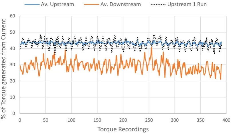
rotational rate of the turbine. The performance of a single model in the channel has been 21

monitored and expressed in terms of torque supplied by current, calculated as a fraction of the 22

recorded torque during the experiments to the required torque in still water. The performance 23

10 between upstream and downstream turbine with a downstream spacing of 12D during array 1

tests. Similarity of rotor geometry and ambient flow conditions to previous experiments and 2

good agreement of the performance indicators give reasonable confidence in the operating 3

conditions in the absence of thrust measurements from the experiments. For all comparisons 4

presented here, diameter and reference pitch angle of the turbine blades were kept constant. 5

The vertical support tower is of elliptical shape to minimize flow disturbance (Mason-Jones 6

et al., 2013) with a length of 0.12m and a maximum width of 0.06m equalling the diameter of 7

the nacelle. The time averaged wake recovery downstream of the vertical support is shown in 8

Fig. 4. The initial transverse extent of the wake is similar to the width of the support and the 9

velocity deficit at the centre line reduces to less than 5% within 1.5D downstream of the 10

support. Flow measurements with two LaVision ImagerProX11M CCD cameras were 11

conducted at 6 locations throughout the wake, starting at 3D downstream of the upstream 12

turbine down to 20D at the end of the test section. A double pulsed YAG laser located 13

underneath the wake centre line on a traversing unit for accurate positioning, with output 14

energy of 425mJ/pulse at 532 nm wavelength was used to illuminate the particles.For each 15

test and measurement location across the test section, 500 double frame/double exposure 16

images have been recorded over a period of 110 seconds corresponding to a minimum of 200 17

rotations of the turbine. 18

11 1

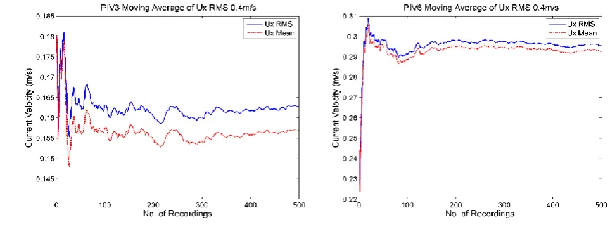
Fig. 1 - Experiment measurements of moving averages at location 3D and 6D, within the 2

wake of scaled tidal turbines at 0.44m/s current 3

The wake measurements were judged to be sufficient by monitoring moving averages of flow 4

velocities and RMS values at locations throughout the wake field as shown in Fig. 1 .Images 5

were pre-processed and analysed using LaVision particle image velocimetry (PIV) system, 6

DaVis 8.2.2, with adaptive interrogation window size and shape adjustment based on local 7

seeding density and flow gradients to obtain the resulting flow vectors in flow with large 8

velocity gradients across the vertical section of the wake. Time averaged wake characteristics 9

are presented and compared to numerical results obtained in the study presented here. Further 10

details of the experiments can be found in Nuernberg and Tao (2016) and Nuernberg and Tao 11

12 1

2

Fig. 2 – Torque supplied by current, calculated from control unit torque data for upstream and 3

downstream turbine in current of 0.44m/s averaged over 6 measurement cycles. Dotted line 4

shows single run. 5

6

0 10 20 30 40 50 60

0 50 100 150 200 250 300 350 400

%

of

T

or

q

u

e

gen

er

at

ed

f

rom

C

u

rr

en

t

Torque Recordings

13 Table 1 - Geometry of scaled NREL S814 rotor

1

r/R 0.3 0.4 0.5 0.6 0.7 0.8 0.9 1

Chord length (mm) 42.04 39.05 36.03 33.03 29.53 27.01 24 21

Pitch Angle (Degree) 23.33 15.83 12.33 10.33 8.33 7.93 7.03 6.33

2

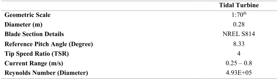
Table 2 - Experiment and Numerical test conditions of scaled tidal turbine arrays 3

Tidal Turbine

Geometric Scale 1:70th

Diameter (m) 0.28

Blade Section Details NREL S814

Reference Pitch Angle (Degree) 8.33

Tip Speed Ratio (TSR) 4

Current Range (m/s) 0.25 – 0.8

Reynolds Number (Diameter) 4.93E+05

The computational domain (Fig. 3(a)) represents the dimensions of the Circulating Water 4

Channel (CWC) at Shanghai Jiao Tong University with a test section extending from -5D 5

upstream of the first turbine location to 22D downstream. Vertically the domain extends 4D 6

from the top-tip of the rotor while the rotor bottom tip to seabed distance is 0.75D. Due to the 7

distance between rotor tip and free surface, and a Froude number of less than 0.2, the 8

computations do not account for the free surface, hence top, side and bottom of the test 9

channel are modelled as no-slip walls, this is also applied to the static parts of the turbine 10

structure. The rotor baldes, hub and cone are modelled as no-slip walls with a moving wall 11

condition to include the rotation according to the operating condition. The current velocity is 12

specified upstream of the array as a velocity inlet on the left and a pressure-outlet is defined 13

on the right, downstream of the array. All rotors are upstream of the vertical support tower as 14

shown in Fig. 3 (b). The inflow was set to an ambient turbulence intensity of 2% through a 15

turbulent kinetic energy (TKE) condition on the inlet patch based on the mean flow velocity 16

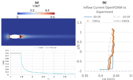
14 A comparison between the numerically achieved velocity profile upstream of the turbine, and 1

the free stream velocity profile measured across the turbine diameter without any devices 2

located in the CWC are shown in Fig. 4 (b), variations between numerical and experimental 3

inflow velocity are small, indicating the present numerical resolution satisfactory. 4

(a) (b)

Fig. 3 – Schematic test section domain with array (L3T15) section inside (a) and model of individual tidal turbine geometry (b)

5

(a) (b)

Fig. 4 – (a) Time averaged velocity deficit (dashed) of vertical support tower at z/D= -0.75 showing the location of the support is shown (solid line) (b) comparison of velocity profile in CWC (without any device in the test section) with achieved inflow at two positions(3D and 1D Upstream of Turbine) in numerical model.

-1 -0.5 0 0.5 1 1.5

0.35 0.4 0.45 0.5

z/

D

Ux (m/s)

Inflow Current OpenFOAM vs Experiment

-3D OF -1D OF

15 Table 3- Boundary conditions used for numerical simulation and wall functions applied 1

Domain Patch Velocity Pressure k ω

Inlet 0.44 m/s Zero Gradient 𝑘 = 1.5 ∗ (𝑈0∗ 𝐼)2 𝜔 = √𝑘/(𝐶𝜇0.25∗ 𝑙)

Outlet Zero Grad 0 Zero Gradient Zero Gradient

Walls (0 0 0) Zero Gradient Zero Gradient (WF) Wall function (3) Rotor & Cone Angular Velocity Zero Gradient Zero Gradient (WF) Wall function (3) Where I is the ambient turbulence intensity (2%) and 𝑙 the inlet mixing length, taken as 0.7 times the diameter (McNaughton et al., 2014).

The tests described in this study include single turbine and multiple turbine set-ups with 3 or 2

4 turbines arranged in a staggered configuration as seen in Fig. 3. Array configurations have 3

been tested for varying longitudinal and lateral spacing between the devices (see Fig. 10). 4

Longitudinal spacing between the first and second array row were varied from 3D to 5D, 5

named as L3 and L5 arrays respectively. Additionally the lateral spacing of the two turbines 6

located in the middle row of the array ranged from 1.5D, 2D and 3D denoted by a T15, T2 7

and T3 respectively. The array names are then a combination of longitudinal and transverse 8

spacing denoted by a combination of the above. The spacing between the first and fourth 9

turbine, both on the array centre line was 12D and is constant throughout all tests. 10

2.2 Numerical Simulation 11

The Finite Volume Method with fluid properties defined at the control volume centroids was 12

used to solve the governing equations. All pre-processing and solving of governing RANS 13

equations is performed in the Open Source software OpenFOAM. The pressure – momentum 14

coupling algorithm used from the OpenFOAM library, PimpleDyMFoam, is a combination of 15

PISO - SIMPLE algorithm allowing for larger time steps (Courant-Friedrichs-Lewy (CFL) > 16

1) in incompressible, unsteady viscous flows as well as dynamic mesh features such as the 17

rotation of turbine blades with a user defined mesh interface between the rotor and stator part 18

of the domain. The solver uses the SIMPLE algorithm to converge the steady state solution 19

16 on the residuals which make the solver advance to the next time step when satisfied, the time 1

step itself is dynamically controlled by a maximum Courant (CFL) number. The 2

computationally more economical RANS approach with the k – ω SST turbulence closure 3

model was chosen based on the previous comparison of RANS and LES simulations with 4

sliding mesh interface by McNaughton et al. (2014) for investigations of tidal turbine 5

performance and wake characteristics. 6

The turbulent kinematic viscosity (υt) wall function is defined in Spalding (1961) with the 7

calculation of local 𝑦+ _{shown in (1), used in OpenFOAM to provide an adaptive wall}

8

function to calculate the friction velocity (uτ) and 𝑦+_{, based on the Newton –Raphson}

9

method (2). These are then used for calculation of turbulence coefficients in the 10

omegaWallFunction (Menter and Esch, 2001), providing omega for viscous and log layer and 11

blending based on 𝑦+_{values in the buffer layer as shown in (3). The OpenFOAM wall}

12

functions are listed in Table 3. Similar to the modelling of a single tidal turbine with sliding 13

mesh by Afgan et al. (2013) average 𝑦+_{values across the tidal turbine blades are less than 5}

14

while vertical support and tower are kept above 30. 15

𝑦+ _{= 𝑢}+₊ 1

𝐸[ℯ𝑘𝑢2− 1 − 𝑘𝑢+− 1

2(𝑘𝑢+)2− 1

6(𝑘𝑢+)3] (1)

16

𝜐_𝑡 = (𝑢𝜏)2

𝜕𝑈 𝜕𝑦

⁄ − 𝜐 and 𝑦

+₌ 𝑢𝜏𝑦

𝜐 and 𝑢𝜏 = √(𝜐𝑡+ 𝜐) (2)

17

𝜔_𝑣𝑖𝑠 =_0.075𝑦6𝜐 ₂ and 𝜔_𝑙𝑜𝑔 = _0.3𝑘1 𝑢𝜏

𝑦 and 𝜔 = √𝜔𝑣𝑖𝑠2+ 𝜔𝑙𝑜𝑔2 (3)

18

17

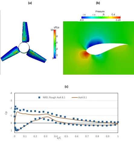
(a) (b)

(c)

Fig. 5 – (a) Dimensionless Y+ across blades structure for array simulations (b) resolved blade 1

shape and pressure coefficient at r/R=0.7. (c) shows comparison with pressure coefficient 2

data at angle of attack of 8.1 degrees from (Janiszewska et al., 1996) conducted with steady 3

inflow and at Re= 750,000. 4

The meshes generated in with OpenFOAMS automated mesh generation utility 5

SnappyHexMesh, are based on a 3D structured hexahedral background mesh, iteratively 6

refined and morphed onto the tidal turbine structure surface by splitting hex-cells that 7

intersect the feature edges and surfaces until the mesh conforms to the boundary.This is 8

followed by removal of all cells within the specified geometry. The final stage snaps the cell 9

vertices onto the surfaces under consideration of mesh quality parameters as described in 10

-4

-3

-2

-1

0

1

0 0.1 0.2 0.3 0.4 0.5 0.6 0.7 0.8 0.9 1

Cp

x/C

18 OpenFOAM 2.3.0 (2014). The resolution of blade section details can be seen in Fig. 5 (b) 1

with local relative pressure around the blade at TSR = 4. Fig. 5 (c) shows the pressure 2

coefficient calculated as shown in (7) from u Liu et al. (2017), computed for the 3D rotating 3

blade using methods described in Johansen and Sørensen (2004) to estimate the local angle of 4

attack and compared to steady flow experiments of a constant blade profile at the same angle 5

of attack, at Reynolds number of 750,000 presented in Janiszewska et al. (1996). Modelling 6

the rotation of the hub, cone and blades is achieved by using the arbitrary mesh interface 7

(AMI), a sliding mesh interface where all cells within the rotational zone rotate at a constant 8

rotation, here set according to the turbine TSR of 4. Care has been taken in the generation of 9

the rotor-stator interface to ensure good overlapping of the source and target patches by 10

generating two identically resolved cylinder surfaces between which the flow information is 11

passed axially and radially. At each rotational step, information is passed between rotor and 12

stator patch interfaces through a cyclic boundary condition with contributions from 13

overlapping cells weighted corresponding to the fraction of overlapping areas. Additionally, 14

the source and target face weights are monitored to avoid introducing conservation errors due 15

to non-conforming patch geometries and monitored to show and average source and target 16

weight sum of 0.99 further information about the implementation of a sliding mesh interface 17

in OpenFOAM can be found in Beaudoin and Jasak (2008). 18

19

(a) (b)

Fig. 6 - Rotor-Stator interface for Rotating AMI zone (a) and mesh density for rotor and 1

stator with AMI interface shown around the rotor (b) 2

A number of meshes with increasing numbers of cells for regional wake refinement have 3

been generated (See Fig. 7 & Table 4). To decrease the computational time for this study, a 4

single turbine mesh configuration was tested in a smaller domain covering a large enough 5

time period to reach at least 20 revolutions of the turbine blades. The different refinement 6

zones of the turbine wake can be seen in Fig. 7 where different cell sizes are used to resolve 7

the wake domain. 8

20 1

Fig. 7 - Tidal Turbine CFD domain with a vertical slice at the centre-line showing wake 2

refinement zones. 3

Table 4 - Mesh Characteristics used for Convergence Study 4

Mesh No. of Cells

Refinement Ratio Approximate cell resolution near blade

Wake cell resolution

Coarse 343698 5.58 x 10-3 _{D 0.089D}

Medium 819607 Coarse - Medium: 1.34

2.79 x 10-3 _{D 0.044D}

Fine 2959484 Medium - Fine: 1.53

0.69 x 10-3 _{D 0.02D}

The obtained mean thrust and power coefficients are compared to numerical experiments and 5

simulations with tidal turbines using a NREL S814 blade section design at TSR = 4. 6

Experiments with same chord and twist distribution with a diameter of 0.4m presented in Shi 7

et al. (2013) were conducted at a blockage ratio of approximately 13% compared to 8

approximately 5% in Milne et al. (2013) & (2015) with near identical chord distribution, and 9

twist angles differing by less than 5 degree except at 0.2r/R where a 10 degree higher blade 10

pitch angle was used by Shi et al. (2013). No blockage correction has been applied, however 11

previous estimates of the effect of blockage in Bahaj et al. (2007) stated a 5% increase of 12

21 The thrust and power coefficient based on calculated torque acting on the turbine blades have 1

been used to determine the discretisation error based on the grid convergence index (CGI) as 2

described in Celik et al. (2008) and shown in Table 5. 3

Thrust Coefficient: 𝐶_𝑇 = 𝐹𝑥

0.5𝜌𝐴𝑈₀2 (4)

4

Power Coefficient: 𝐶_𝑃 = _{0.5𝜌𝐴𝑈}𝑃𝑜𝑤𝑒𝑟

03 (5)

5

Non-dimensionalised Reynolds shear stress: 𝑅𝑑𝑖𝑚 = √_(𝑢̅|𝑢̅̅̅̅̅̅̅|₂′_+𝑤𝑤_̅′₂₎ (6) 6

Pressure Coefficient 𝐶𝑝 = 𝑃0−𝑃∞

0.5𝜌[𝑈2_{+ (𝜔𝑟)}2_] (7) 7

where FX is the time averaged axial force acting on the structure, U0 is the ambient current 8

velocity and A the rotor swept area. The power is calculated from the time averaged axial 9

moment and rotor angular velocity. The time averaged thrust and torque over a period of 20 10

seconds have been used with constant sampling rate between all simulations, showing 11

oscillating convergence. The extent of loading on the vertical support structure is less than 12

5% of the thrust experienced by the entire device. 13

22 Table 5 - GCI of Thrust and Power Coefficient, Comparison to previous numerical and 1

experimental simulation 2

Coefficients

Mesh CT CP

Fine 0.709 0.353

Medium 0.698 0.336

Coarse 0.704 0.341

Extr.(Fine) 0.711 0.342

GCI (%, Med) 2.9 1.57

GCI (%, Fine) 2.5 3.12

3

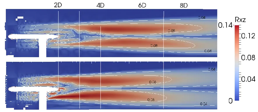
Error estimates for the wake velocity show similar trend to those presented for the wake 4

downstream of an actuator disk modelled in combination with BEMT by Batten et al. (2013) 5

between 4D and 10D, however a much higher GCI is observed at 6D and 7D. Based on the 6

obtained GCI values, additional comparison of non-dimensionalised Reynolds shear stress (6) 7

maps is performed between the medium and fine mesh configuration and additionally to 8

experiments conducted at CT = 0.79, CP = 0.43 and TSR = 3.67 with ambient turbulence 9

intensity of 3% by Mycek et al. (2014a) providing detailed flow field information at similar 10

low turbulence conditions, with a different blade section profile, to investigate the 11

approximate location of the merging of the upper and lower mixing layers. Fig. 8 shows the 12

interaction of the upper and lower mixing layer between 4D and 7D comparing well to those 13

reported in experiments. By comparing the medium (top) and fine (bottom) mesh, it can be 14

seen that the medium mesh shows good agreement with the fine mesh in most regions of the 15

wake, more detailed mixing can be observed in the near wake of the fine mesh. Around 6D 16

and 7D the shape of the mixing layers in the averaged contour plots shows more variations in 17

the medium mesh than the fine mesh, which could be a reason for the varying GCI values 18

obtained. Differences in resulting velocities between the two meshes are around 10% in the 19

near wake reducing to 6% by 8D, for a 100% increase in computation time of the fine mesh. 20 This Study(Num/Exp) Shi (Num/Exp) Milne (2013 / 2015) Mycek Blockage ratio

1.3 % 13 % 5 % 4.8%

CP 0.34/0.43* 0.35 / 0.43 0.38 /

0.35

0.43

CT 0.70* 0.72 / 0.95 0.77 /

0.56

0.79

23 1

Fig. 8 - Normalised Reynolds shear stress map: comparison of medium (top) and fine 2

(bottom) mesh. 3

Table 6 - Discretisation error estimation using GCI, flow of 0.44m/s and TSR 4 4

Time-averaged in-stream Velocity, Ux (m/s)

2D 3D 4D 5D 6D 7D 8D 9D 10D

Fine 0.0241 0.220 0.234 0.267 0.296 0.317 0.332 0.342 0.350

Medium 0.0254 0.211 0.211 0.231 0.262 0.290 0.312 0.327 0.339

Coarse 0.0245 0.235 0.220 0.232 0.248 0.265 0.280 0.293 0.303

Extrapolated (Fine)

0.0206 0.237 0.253 0.336 0.36 0.367 0.343 0.371 0.352

GCI (%, Med) 10.12 0.03 7.52 0.18 18.85 38 12.5 7.6 4.74

GCI (%, Fine) 1.42 0.19 10.4 1.54 25.9 25 4.2 1.73 0.66

5

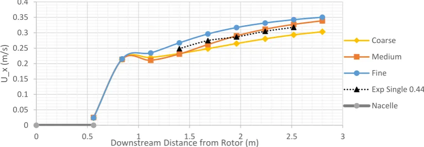
Additionally, the mesh configuration for turbine structure and flow domain was investigated 6

by comparing the time-averaged in-stream velocity at different downstream stations along the 7

rotor centre-line to the values recorded in the experimental study shown in Fig. 9. 8

Comparison to experimentally measured flow values shows the medium and fine mesh have 9

best agreement along the wake centre-line. The experimental velocity recordings are within 10

less than 10% difference of the numerical values obtained during the mesh sensitivity study. 11

The fine mesh approximately over predicts the wake recovery by 8% through the wake region 12

tested. The medium mesh under predicts the recovery up to 7D downstream, in agreement 13

24 and medium mesh, and slightly over predicts in-stream velocity component thereafter. Based 1

on the presented investigation, the medium mesh is chosen to reduce the computational cost 2

when applying mesh settings on full array configuration where domain sizes varied from 1.5 3

million to 4.2 million cells, with closer lateral spacing leading to higher number of cells 4

during the automated mesh generation. The agreement in terms of loading and with 5

experimental values from the present and other studies mentioned, gives reasonable 6

confidence in the applied mesh for initial comparison to experiments and to gain insights into 7

the wake structure in closely spaced tidal turbine arrays. 8

9

Fig. 9 - Time averaged Numerical vs Time averaged Experiment Data for in-stream velocity 10

component across a number of meshes. 11

12

0 0.05 0.1 0.15 0.2 0.25 0.3 0.35 0.4

0 0.5 1 1.5 2 2.5 3

U

_x

(m

/s

)

Downstream Distance from Rotor (m)

Coarse

Medium

Fine

Exp Single 0.44

25

3.

Results and discussion

1

The numerical simulations presented are compared to experimental measurements previously 2

conducted in a circulating water channel. Therefore data is obtained according to the same 3

recording interval used for the 500 PIV images during the experiment, corresponding to a rate 4

of 4.52Hz for comparison of average flow characteristics. Time averaging of all flow 5

characteristics is performed at run-time for each time step (in the order of 1.5 - 3 x 10-3 6

seconds), thus the averaged data sampled here includes effects of all periodic fluctuations 7

occurring at higher frequencies. 8

The numerical simulations presented here are primarily performed for comparison with 9

existing experimental measurements and to present a numerical investigation using 10

opensource software capabilities and automated mesh generation. Further numerical 11

investigation and improvement of the current model will be perfomed to improve the 12

correlation between the experimental and numerical cases. This will allow further and more 13

detailed investigation of the resulting flow field as a result of the micro arrangement of tidal 14

turbine devices arranged in arrays. The definittion of array cases are provided with reference 15

to Fig. 10, where the longitudinal distance between the first and second row of turbines (R1) 16

is varied from 3D to 5D denoted as L3 and L5 respectively. The third row of turbines is 17

always located 12D downstream of the first row. Transverse spacing (S) is denoted as T15, 18

T2 and T3 to identify each combination tested. 19

Firstly the wake of a single turbine arrangement will be compared to the wake obtained from 20

PIV measurements.The numerical results of a number of different array sections are then 21

compared to the experimental results of arrays with varying longitudinal and lateral inter-22

26 numerical data. Data is presented in terms of time averaged in-stream wake velocity deficit 1

(1- U/U0) and turbulence intensity . 2

3

Fig. 10 - Definition of Array cases: R1 is denoted as L3 or L5 whereas S will be given either 4

T15, T2 or T3. 5

3.1 Comparison with Experiments

6

The velocity and turbulence characteristics are compared to those recorded during the 7

experimental study. Between 9D and 14D no measurements were taken during the 8

experiment due to obstruction of the PIV equipment by a steel frame between the observation 9

windows of the test section. Where the centreline measurements were taken for the position 10

of the second row (at 3D and 5D downstream respectively) no measurements could be 11

obtained for the close lateral spacing of 1.5D in the PIV due to the presence of the tidal 12

turbine. No data is obtained in the numerical simulation between 12D and 14D due to the 13

location of the downstream turbine. Further investigation of the flow characteristics follows 14

this comparison. 15

16

A

B

C

27

Single Turbine 0.44 m/s

(a) (b)

Fig. 11 - Comparison between numerical simulations (solid line) and experiment 1

measurements (box) for a Single turbine operating in ambient flow of 0.44m/s: Velocity 2

deficit (a) and turbulence intensity (b). 3

The agreement between numerical simulations and experimental measurements varies 4

depending on the location and configuration of the conducted tests and corresponding 5

numerical simulation (Fig. 11 - Fig. 13). The wake characteristics of a single turbine 6

presented in Fig. 11 (a) show good agreement between 5D and 9D, thus within range of 7

placing the second-row turbine. The velocity deficit downstream (14D-20D) matches well 8

with that measured during experiments. The rate of velocity recovery observed between 7D 9

and 15D is very similar and a remaining velocity deficit of 13% is observed for both at 20D. 10

The turbulence intensity is over predicted in the near wake of the tidal turbine (x/D < 5), the 11

trend of dissipation of turbulence towards free stream levels as well as the location of 12

maximum turbulence intensity are similar, yet differ in magnitude by approximately 7%. In 13

the far wake region between 15D – 20D good agreement is shown, with a remaining 14

turbulence intensity between 5% - 7% at the centerline height of the tidal turbine thus not 15

recovering towards free stream levels within 20D. Further downstream the numerical 16

turbulence intensity remains slightly higher than ambient turbulence (5% at 20D) whereas in 17 0 0.2 0.4 0.6 0.8 1

0 3 6 9 12 15 18

V elo cit y D ef ic it (1 -Ux /U) x/D

Vdef Exp Vdef Sim

0 20 40 60

0 3 6 9 12 15 18

Turb u len ce In te n sity (% ) x/D

28 the experiment the turbulence intensity recovers to about 7% at 20D. The increase in

1

turbulence intensity observed in both cases, reaching a peak between 4D and 5D shows the 2

location where centre line wake recovery accelerates. Differences are most pronounced in the 3

near wake close to the support structure where high velocity gradients and stagnating flow 4

was observed in the experiment, thus increasing the difficulty of ensuring appropriate time 5

stepping of PIV measurements. The numerical simulations showed accelerated flow around 6

the turbine hub followed by the wake expanding towards the centre line, thus explaining the 7

increase in velocity deficit between 2D and 4D. 8

Comparing the array centre line velocity deficit and turbulence characteristics at hub height 9

shows better agreement across the array formations (Fig. 12 & Fig. 13) than the isolated 10

turbine. Some significant differences between experiment and numerical simulation are 11

observed immediately downstream of the turbine, where due to high velocity shear across the 12

wake, calculation of flow vectors using PIV was difficult and further calculation of 13

turbulence intensity for very slow flow velocities resulted in high values compared to the 14

numerical solution. However, the velocity deficit (a) shows better agreement in the wake 15

downstream of last row of turbines whereas the turbulence intensity (b) for the close 16

arrangement of tidal turbines in a staggered array is agreeing well within the array section 17

itself, between 2D and 9D. The increasing velocity deficit downstream of the second row of 18

turbines is observed in experiments and numerical simulation for both array cases. For 19

L3T15, the experiments show a near constant velocity deficit between 5D and 7D and 20

numerical results (Fig. 12(a)) indicate an increase in velocity deficit by 8% for L3T15 21

between 4D and 6D. The wake recovery downstream of the last row of turbine is increased 22

for L3T15 in the experiments between 15D and 18D however, the final velocity deficit 23

remaining in the wake at 20D downstream differs by only 3%. For the increased longitudinal 24

29 wake downstream of the last turbine. The increase in velocity deficit downstream of the 1

second row turbines is also observed for the longitudinal spacing of 5D as can be seen in Fig. 2

13 (a) between 6D and 9D. Flow recovery downstream of the last row is almost identical with 3

differences in the velocity deficit of approximately 2%. The turbulence intensity within the 4

array is predicted well within (4D-9D) the array as seen in Fig. 13(b). The dissipation of 5

downsteam turbulence is slower in the numerical simulation than in the experiments recorded 6

and a higher turbulence remains at 20D. 7

One reason for the differences is an observed shift in the wake centreline due to higher shear 8

at the upper wake boundary in the experiments. This has not been shown in the numerical 9

simulation and could be influenced by the omission of the small support frame used in the 10

experiment that effectively increased the roughness of the test section floor which led to less 11

mass flow at the underside of the wake as was shown by (Myers and Bahaj (2010)) for 12

actuator disk experiments. In a low ambient turbulence environment the developing wake 13

from the support reduced wake mixing on the lower part of the wake, thus slowing down 14

recovery of velocity when compared to numerical modelling where flow is passing between 15

the bed and turbine wake as will be shown. 16

17

30

L3T15 Array

(a) (b)

Fig. 12 - Velocity deficit (a) and turbulence intensity (b) comparison between numerical 1

simulations (solid line) and experiment measurements (box) for the L3T15 array operating in 2

ambient flow of 0.44m/s 3

L5T15 Array

(a) (b)

Fig. 13 - Velocity deficit and turbulence intensity comparison between numerical simulations 4

(solid line) and experiment measurements (dashed) for the L5T15 array in ambient flow of 5 0.44m/s 6 7 0 0.2 0.4 0.6 0.8 1 1.2

0 3 6 9 12 15 18 21

Ve locity De fici t (1 -U x/U ) x/D

Vdef Exp Vdef Sim

0 20 40 60

0 3 6 9 12 15 18 21

Tu rb u le n ce In ten sity (% ) x/D

Ti Exp Ti Sim

0 0.2 0.4 0.6 0.8 1 1.2

0 3 6 9 12 15 18 21

Ve locity De fici t (1 -U x/U ) x/D

Vdef Exp Vdef Sim

0 20 40 60

0 3 6 9 12 15 18 21

Tu rb u le n ce In ten sity (% ) x/D

31 While the turbulence intensity is matched well in the inner array section the velocity deficit 1

shows better agreement for the downstream wake region. The inner array region is where 2

device generated turbulence dominates and the influence of not including the support frame 3

in the numerical model is less pronounced. Matching the turbulence intensity within the array 4

improves the prediction of the centreline velocity recovery downstream of the array. The 5

wake downstream of the array differs in terms magnitude of turbulence intensity could be 6

caused by the turbine wake reaching towards the bottom of the test tank, thus reduced mixing 7

occurs and the wake is observed further downstream of the array. 8

3.2 Wake characteristics from CFD 9

Comparison of array wake characteristics across the two longitudinal spacings of L3 and L5 10

are shown in Fig. 14 (a) and (b) respectively. Close lateral spacing (T15) showed a higher 11

remaining velocity deficit for a longer downstream distance within the array section for both 12

longitudinal spacings tested. Two diameters downstream of the second turbine row, the 13

velocity deficit is highest for T15 and lowest for T2, downstream of this point the recovery 14

rate is slower for T15 than for T2 & T3 with the wide lateral spacing of T3. The velocity 15

deficit upstream of the last turbine is reduced by 3 - 8% for configuration T2 & T3 by 16

increasing the longitudinal separation of the first two rows from 3D to 5D. There is little 17

difference for the inflow to the last turbine for the close lateral spacing of T15 with a velocity 18

deficit of almost 50% one diameter upstream. For T2, little recovery is observed between 6D 19

and 8D at the array centre line. For transverse spacing of T3 steady wake recovery is 20

observed up to 11D before an increase in velocity deficit of 8% between 1D and 0.5D 21

upstream of the last turbine can be seen in shown in Fig. 15. Downstream of the array the rate 22

of wake recovery is very similar with the T3 cases showing slightly accelerated recovery and 23

32 1

Array Comparison

(a)

(b)

Fig. 14 - Comparison of wake velocity deficit for arrays with longitudinal spacing of L3 (a) 2

and L5 (b). 3

4

0.0 0.2 0.4 0.6 0.8 1.0 1.2

0 3 6 9 12 15 18 21

Ve

locity

De

fici

t

(1

-U

x/U

)

x/D

L3

L3T15 L3T2 L3T3

0 0.2 0.4 0.6 0.8 1 1.2

0 3 6 9 12 15 18 21

Ve

locity

De

fici

t

(1

-U

x/U

)

x/D

L5

33 1

Fig. 15 - Comparison of velocity deficit at array centre line between L3T3 and L5T3 2

Comparison of the centre line velocity deficit on the vertical plane (xz) for L3 arrays (Fig. 3

17) shows an area of reduced deficit just downstream of the second row rotors for T15 and 4

T2 in (a) and (b) respectively, where the ambient current is flowing towards the array center 5

line due to the increased blockage of the two rotors thus reducing the velocity deficit. 6

Downstream of the second row turbines a stronger velocity deficit is seen. The vertical array 7

centre line shows that the transverse spacing influences the vertical characteristics of the 8

wake with a more pronounced area of slow moving fluid being present and larger variations 9

of the velocity deficit across the rotor height ranging from 20% to 45 %. This will influence 10

the performance and optimum tuning of downstream turbines operating in a highly varying 11

flow field across the rotors 12

The thrust and power coefficients for all turbines are presented in Table 1, performance data 13

for the downstream turbine has been calculated based on the array inflow conditions (U∞) 14

and the predicted inflow velocity one diameter upstream of the turbine, averaged across 15

circular elements across the turbine diameter. From the presented data it can be seen that 16

while the operation of the first turbine is constant across all configuration, the second row 17

34 power coefficients when close to or operating in part of the upstream wake. The performance 1

of the downstream turbine is significantly reduced, as expected due to operating off design 2

point (TSR=4) with an effective TSR of 5.4 to 6.5 due to the slowed inflow conditions. 3

Table 7 - Comparison of operating conditions of turbines in array, velocity upstream of array 4

(U∞) and 1D upstream of last turbine are used for calculation of tip speed ratio, thrust and 5

power coefficient of downstream turbine (D), definitions of turbine are shown in Fig. 10.The 6

TSR is 4 for all turbines facing ambient flow, and the effective TSR for the downstream 7

turbine has been included. 8

Single L3T15 L3T3 L5T15 L5T3

Turbine CT CP CT CP CT CP CT CP CT CP

A 0.7 0.34 0.70 0.33 0.70 0.32 0.70 0.33 0.70 0.33

B 0.62 0.27 0.71 0.30 0.64 0.29 0.74 0.38

C 0.63 0.25 0.70 0.32 0.65 0.29 0.74 0.35

D

Effective TSR 6.3 5.4 6.5 5.4

Array (𝑈∞) 0.36 0.04 0.43 0.09 0.34 0.02 0.46 0.11

U1D Upstream 0.9 0.13 0.79 0.19 0.95 0.08 0.65 0.23

9

The differences in the resulting wake field within and downstream of the array can be 10

observed from Fig. 16. With closer lateral and longitudinal spacing (a), the flow field shows a 11

combined wake without ambient flow between the adjacent turbine wakes. An area of slow 12

moving fluid, about 1D wide, can be seen at the array center line downstream of row two. 13

The initial wake of the first turbine contracts between the rotors of the second row and is less 14

pronounced in the near wake, however the velocity deficit increases further downstream as 15

shown previously in Fig. 14. For the increased turbine separation the initial wake develops 16

behind the turbine structure showing an increased velocity deficit but faster recovery 17

35 individual wakes can be clearly identified. Downstream of the array, a larger velocity deficits 1

persists in the transverse direction. 2

3

36 1

37 The transverse wake velocity deficit profiles at three different stations for all 6 configurations 1

are shown in Fig. 18 showing wake development and dissipation across the transverse domain 2

at hub height. With transverse spacing of T15 a single wake is identified for L3 at 8D and 3

10D with the highest velocity deficit at the centre line and the profile resembling a bell 4

shaped curve. For T2 and T3, individual wakes are identified and it can be seen that increased 5

mixing with the ambient flow occurs in T3 up to 10D at y/D > 0 where the velocity deficit of 6

the free stream between the wakes is increased compared to y/d <0. This could indicate a 7

slight movement of the wake towards the y/D >0 side which is in the direction of wake 8

rotation (the turbine blades are rotating anti-clockwise direction when looking from the 9

upstream direction towards the array). Downstream of the array T15 and T5 transverse 10

spacing result in a single, combined wake where the T2 wake is wider, more pronounced so 11

in the L3 arrays than L5. For T3 spacing, three individual wake exist downstream of the last 12

turbine and increased velocity deficits can be observed in y/D > 0. The peak velocity deficits 13

in the combined or individual wakes do not differ significantly in terms of velocity deficit. 14

The similarities of the downstream wake recovery were observed in experiments as well. 15

A comparison of the variation of Reynolds stresses in the x-y plane at different downstream 16

distances from the second row of turbines is shown in Fig. 19. The existence of a large area 17

of slow moving fluid in L3T15 as shown in Fig. 16 (a) results of little mixing within the array 18

wake (a) from -1D to 1D transversely from the rotor center at 3D downstream. At 5D 19

downstream of the second row the mixing layers are wider and show only the outer mixing 20

with ambient current around the array. For increased separation, increased mixing can be 21

observed and individual peaks corresponding to the respective turbines located in the array 22

are clearly shown. Downstream of the array (b) the differences are less pronounced, but for 23

close transverse spacing a diffuse mixing layer is observed whereas individual layers can be 24

38 1

Fig. 18 - Array transverse profiles of velocity deficit T15 (solid), T2 (dash) and T3 (cross)

2

3

4

39 A comparison of the turbulence intensity as calculated from the numerical results is shown in 1

Fig. 20. Increased turbulence can be seen downstream of the second row of rotors (a) with the 2

dissipation being faster on the upper part of the wake compared to the lower part. The 3

transverse turbulence intensity (b) shows increased levels around the turbine support 4

structures and in the near wake of the rotors and higher levels in areas where the velocity 5

recovery rate is increased. For the inner array wake, turbulence intensities are high at low 6

current velocities, however the mixing in the fluid is slower as shown previously which 7

despite the large intensities observed in (b) results in slower wake recovery for the L3T15 8

array. Similar to the wake velocity deficit, separate wakes can be observed for increased 9

lateral spacing and slightly increased intensities are shown in (c) where the velocity deficit 10

was shown to contract between the two second row turbines. 11

The reduction in transverse wake extent, which is more pronounced in the arrays with L5 12

spacing in Fig. 16(b) where the wake had further downstream distance to expand before 13

flowing between the second row turbines at 5D occurs around the location where vortices are 14

shed by the second row turbines which are visualised by the Q-criterion in Fig. 21. The 15

vortices cause extrac blockage by increaseing the wake area and the ambient flow between 16

the initial wake and the second row turbines leads to smaller transverse wake extent at this 17

area.The breakdown of vortices occurs within 2D downsteam of the individual rotors and 18

within about 1D for the last row turbine. The area of high velocity deficit observed on the 19

side of the first and second row turbines shows an additional wake due to the vertical support 20

strucutre of the turbine blocking rotating flow around the nacelle. Upstream of the vertical 21

support the distance between adjacent vortices reduces before vortices break down at the 22

vertical support and then expands downstream of the support followed by rapid break down 23

40 3D downstream of 2nd _{Row Rotor 5D downstream of 2}nd _Row

3D downstream of last turbine 5D downstream of last turbine

Fig. 19 - Transverse profiles of Reynolds Stresses (xy) for L3T15 (dot), L3T3 (dash), L5T15 (solid) and L5T3(dash dot)

-3 -2 -1 0 1 2 3

-0.0020 0.0000 0.0020

y/D

-3 -2 -1 0 1 2 3

-0.0020 0.0000 0.0020

y/D

-3 -2 -1 0 1 2 3

-0.0020 0.0000 0.0020

y/D

-3 -2 -1 0 1 2 3

-0.0020 0.0000 0.0020

41 1

42 1

Fig. 21 - Velocity deficit and Q-criterion (Q=2) for propagation of vortices around the turbine 2

support structure in L5T3 array 3

43

4.

Conclusion

1

The comprehensive CFD study presented here showed the applicability of transient RANS 2

simulations with a rotor-stator interface to account for the effects of rotating tidal turbine 3

blades and the flow field characterisation in tidal turbine arrays. Three dimensional RANS 4

simulations with the k – ω SST turbulence model have been compared to data from 5

experimental measurements and shown reasonable agreement for a single turbine and within 6

the array sections tested. Further improvements to the numerical set-up are required to 7

achieve better agreement across the whole fluid domain, through thorough investigations of 8

the effects of mesh refinement across different zones of the wake domain and the inclusion of 9

the effects of the support frame which was used in the experimental study. Differences in the 10

vertical shift of the wake are attributed to this structure. Simplified methods of applying 11

appropriate wall roughness instead of modelling a support frame may aid in overcoming the 12

difficulties of modelling this complex support arrangement in automatic mesh generation. 13

Using openly available software with automatic mesh generation for numerical simulation of 14

tidal turbine arrays showed that with increasing computational resources available these 15

studies can be performed on reasonably sized workstations as all computations shown here 16

where run on a maximum number of 32 cpu cores. 17

Brief investigation of the complicated flow field has highlighted the existence of zones of 18

flow acceleration and ambient flow adjacent to multiple turbine wakes when turbines are 19

installed in close proximity and given some insight to the wake recovery in low turbulence 20

ambient flow and under different longitudinal and transverse spacing. By varying the inter-21

device spacing in both longitudinal and transverse direction, the wake characteristics within 22

44 The transverse spacing determines whether adjacent wake combine within the array section, 1

which was observed for a combination of close longitudinal and transverse spacing (L3T15 & 2

L5T15). Both configuration using very close transverse spacing have shown slow, and 3

stagnant wake recovery within the array section and large areas of high velocity deficit, 4

however the effect on the overall array wake was less pronounced in terms of final velocity 5

deficit. It was shown that by closely arranging tidal turbines, reduced mixing occurs within 6

the wake when the outer and inner wake of tidal turbines block all ambient flow between 7

them, which led to the slow rates of wake recovery. By increasing both inter-device 8

distances, ambient flow is observed between the individual wakes which increases the wake 9

recovery of the array centre line and leads to the individual wakes being identifiable. 10

Turbines operating in wake of upstream turbine showed faster recovery due to increased 11

turbulence, hence mixing with the ambient flow. The exact extent of this also depends on the 12

operating conditions of the turbine which was presented in terms of the inflow conditions to 13

the array and downstream turbine, and no adjustment to individual inflow characteristics of 14

the downstream turbine were made here, meaning that the last turbine operated at increased 15

TSR. 16

Further three dimensional analysis of the numerical results gave a brief insight into the 17

shedding and breakdown of vortical structures around the turbine hubs. The breakedown of 18

vortices occurs just downstream of the turbine structure for the turbines operating in 19

unaffected flow. The area of breakdown of vortices is located upstream of the area where 20

transverse wake expansion occurs linked to the onset of the expanding shear layer towards 21

the centre line of the wake. 22

With further improvement and overcoming the limitations mentioned, automatic mesh 23

45 the rotating turbine blades can therefore be used for investigation of the complex flow

1

characteristics within a tidal turbine array to further investigate the layout and micro spacing 2

of devices in commercial arrays. 3

46

Acknowledgment

1

This work made use of the facilities of N8 HPC Centre of Excellence, provided and funded 2

by the N8 consortium and EPSRC (Grant No.EP/K000225/1). The authors gratefully 3

acknoledge the support received in conducting experiments at the School of Naval 4

Architecture, Ocean and Civil Engineering at Shanghai Jiao Tong University and the British 5

Council (China) under the “Sino-UK Higher Education Research Partnership” as well as 6

LaVision for providing support and software for the PIV analysis. 7

References

Abolghasemi, M.A., Piggott, M.D., Spinneken, J., Viré, A., Cotter, C.J., Crammond, S., 2016.

9

Simulating tidal turbines with multi-scale mesh optimisation techniques. Journal of Fluids and

10

Structures 66, 69-90.

11

Afgan, I., McNaughton, J., Rolfo, S., Apsley, D.D., Stallard, T., Stansby, P., 2013. Turbulent flow and

12

loading on a tidal stream turbine by LES and RANS. International Journal of Heat and Fluid

13

Flow 43 (0), 96-108.

14

Ahmadian, R., Falconer, R.A., 2012. Assessment of array shape of tidal stream turbines on

hydro-15

environmental impacts and power output. Renewable Energy 44, 318-327.

16

Atlantis Resources Ltd, 2016a. MEYGEN UPDATE – FULL POWER GENERATION FROM

17

TURBINE #1,

https://atlantisresourcesltd.com/2016/12/07/meygen-update-full-power-18

generation-turbine-1/.

19

Atlantis Resources Ltd, 2016b. NICOLA STURGEON, FIRST MINISTER OF SCOTLAND,

20

UNVEILS WORLD’S LARGEST FREE STREAM TIDAL POWER PROJECT,

21

https://atlantisresourcesltd.com/2016/09/13/nicola-sturgeon-first-minister-of-scotland-unveils-22

world-s-largest-free-stream-tidal-power-project/.

23

Bahaj, A.S., Molland, A.F., Chaplin, J.R., Batten, W.M.J., 2007. Power and thrust measurements of

24

marine current turbines under various hydrodynamic flow conditions in a cavitation tunnel

25

and a towing tank. Renewable Energy 32 (3), 407-426.