A fully nonlinear numerical method for modeling wave-current interactions

City, University of London Institutional Repository

Citation

: Wang, J., Ma, Q. ORCID: 0001-5579-6454 and Yan, S. ORCID:

10.1016/j.jcp.2018.04.057

This is the accepted version of the paper.

This version of the publication may differ from the final published

version.

Permanent repository link:

Link to published version

: http://dx.doi.org/10.1016/j.jcp.2018.04.057

Copyright and reuse:

City Research Online aims to make research

outputs of City, University of London available to a wider audience.

Copyright and Moral Rights remain with the author(s) and/or copyright

holders. URLs from City Research Online may be freely distributed and

linked to.

City Research Online: http://openaccess.city.ac.uk/ [email protected]

* Correspondence to: Northampton Square, Goswell Road, London, EC1V 0HN, UK

E-mail address: [email protected]

A Fully Nonlinear Numerical Method for

Modelling Wave-Current Interactions

Jinghua Wang, Q.W. Ma*, Shiqiang Yan

School of Mathematics, Computer Science and Engineering, City University of London, United Kingdom

Abstract

The presence of current in the ocean can significantly modify the characteristics of ocean waves, and it

is considered as an important factor responsible for the occurrence of extreme waves, e.g., rogue waves,

which are well known as great threats to ocean engineering practices. The magnitude and direction of ocean

current normally vary spatially and ocean waves can become very large and steep. Accurate and efficient

phase-revolved numerical methods of fully nonlinear wave-current interactions on a large scale in three

dimensions (3D) are required to understand their properties, but the existing phase-revolved methods are

all based on the assumption of linear or weakly nonlinear interactions. This paper will address the issues

and present a fully nonlinear numerical method to model the 3D interactions between waves and varying

current on a large scale using a phase-revolved formulation. A new set of equations describing the

three-dimensional, fully nonlinear interactions between waves and horizontally shearing current is proposed.

They are derived by making no assumption on wave steepness or the order of wave-current interaction. The

resulting new equations correctly describe the free surface boundary conditions by representing the fully

nonlinear wave-current interactions, removing the limitation to the small wave steepness of the existing

formulations in literature.

On this basis, the recently developed Enhanced Spectral Boundary Integral (short as ESBI) method is

further enhanced to be able to model the wave-current interactions using the new equations, by developing

the appropriate procedure for dealing with the extra terms related to nonlinear wave-current interactions.

The new equations are used as the prognostic equations for updating the free surface in time domain, and

a fast converging iterative technique is employed to solve them. The robustness of the newly developed

method is demonstrated through comparing with experimental data available in literature and good

waves and horizontally varying current. A comparison with a Higher Order Spectrum (HOS) method based

on weak-nonlinear formulation of wave-current interaction is also made to confirm larger error does appear

if the wave steepness is large. The method presented in the paper can be employed to simulate the real

evolution of ocean waves on current in a phase-revolved way to give deep insights to the dynamics of

wave-current interactions, which may not be done correctly by the existing methods so far.

Keywords: Wave-current interaction; Enhanced Spectral Boundary Integral method (ESBI); Random Seas; Rogue waves; Deep water; Large scale modelling; horizontally varying current, fully nonlinear simulation.

1

Introduction

When ocean waves encounter current, their properties, e.g., direction, speed, wave length and height,

will be significantly modified. The current may affect the wave condition and increase the probabilities of

the rogue wave occurrence [1], which are extreme waves of twice the significant wave height. Due to their

abnormal dynamic features distinguished from the surrounding waves, rogue waves can impose great

uncertainties on the safety of human’s oceanic activities. Studies have pointed out that the ship accidents

near the Agulhas current may be associated to the wave-current interactions [2, 3]. More recently, Lavrenov

& Porubov [4] suggested that there are at least three reasons for rogue wave occurrence due to presence of

current, i.e., a) wave energy amplification due to wave-current interaction, b) wave height amplification

around a caustic due to refraction, and c) non-linear wave interaction in shallow water due to intersection

of waves moving from different directions reflected by current. Therefore, accurate modelling of

wave-current interactions is very important for the understanding of rogue wave mechanisms. In order to perform

forecast and prevent impacts in advance in engineering practices, developing an efficient and accurate

numerical tool to model wave-current interactions can be beneficial in practical perspective.

In many instances, the time and length scales of current are much larger than those of the waves, hence

it is natural to assume the current is uniform in a local area [5]. To look at the local effects, many theoretical

studies have investigated the interactions between a regular wave train with the uniform current [5-11], and

good reviews can be found in [5] and [12]. Efforts have also been made to extend that to study the interaction

(NWTs) are developed, e.g., those based on the shallow water equations [13-17], fully nonlinear Boundary

Element Method [18-22] and Quasi-Arbitrary Lagrangian-Eulerian Finite Element Method [23], Fast

Fourier Transform (short as FFT) based fully nonlinear Higher Order Spectrum (short as HOS) method [24]

and Spectral Boundary Integral (short as SBI) model [25], and those based on the coupled continuity and

Navier-Stokes equations [26-28].

Despite the success of those models for simulating the interactions between waves and the uniform

current, the variation of the current in space cannot be considered by using them. The spatially varying

current is often observed in real ocean environment and plays very important role in wave propagation on

large scale, e.g., the large-scale variation of a current can change all the parameters describing a wave train

as indicated by Peregrine [5]. To study the effects of varying current, the linear ray theory [29] is suggested,

which can accurately predict the changes in wave length and direction due to refraction and blocking.

However, it cannot predict the changes in the wave amplitude because waves become essentially nonlinear

at the blocking point and therefore the linear solution is no longer accurate [22]. Although nonlinear theories

describing the progressive waves riding on varying current are suggested [30-33] and fruitful results have

been reported in recent studies [34-41], they can only be applied to regular waves or modulated uniform

wave train [41], therefore such models are insufficient to describe random ocean waves consisting of

components covering a wide range of spectra and subjected to spatially varying current. Nevertheless, an

effective way to model random waves on varying current is through the phase-averaged models, which can

provide useful statistical information, such as the spectra, etc. [42]. However, the specific wave kinematics

and dynamics cannot be provided by the phase-averaged models due to the lack of the phase information,

which are of great importance for precisely evaluating the responses and survivability of marine structures

in real seas. Thus, the models in a phase-resolved approach are required.

Several phase-resolved models have been proposed. For example, the so-called Non-Linear Schrödinger

Equation (short as NLSE) has been employed to study the current generated by a relatively small-amplitude

slowly-varying internal long wave [43-48]. By using that, the effects of non-uniform current on the

probability of rogue waves are explored, and it is found that the opposing current can cause rapid instability

[46, 47]. Nevertheless, the NLSE is derived by assuming small wave steepness and narrow bandwidth,

otherwise it becomes less accurate when applied beyond the limitations. The suitability of the NLSE for

modelling random waves is discussed by Wang, et al. [49], in which the error of the NLSE has been

quantified for simulating random waves. Due to such limitations, the NLSE will not be adopted in this

study.

To avoid such drawbacks, the HOS method has been extended to consider the effects of slowly varying

current in a weakly rotational media [50]. However, the formulations of this model are derived by expanding

higher order nonlinear terms. Although the method overcomes the limitation of narrow bandwidth imposed

on the NLSEs, it is essentially weakly nonlinear for modelling wave-current interactions, and becomes less

accurate when being used to simulate large steepness waves (more details will be given in the next section).

As restated, robust numerical modeling of wave-current interactions on large scale in two and three

dimensions, while considering sufficient nonlinearities, can be useful to both applied science and

engineering practices. However, the existing numerical models lack at least one of the following features:

(i) modelling both regular and irregular waves in presence of current; (ii) simulating the current field that

may be uniform or varying in space; (iii) being fully nonlinear and unassuming small wave steepness or

narrow spectral bandwidth; (iv) being computationally efficient on large scale in both two and three

dimensions. So far, the numerical method that can model the fully nonlinear interactions between waves

and varying current on large scale in both two and three dimensions, possessing all the above features, has

not been proposed to the best of the authors’ knowledge. Therefore, to accurately model the effects of

varying current on wave propagation on large scale becomes challenging due to the lack of such a powerful

tool. This study successfully overcomes this challenge through three breakthroughs:

i) A new set of equations describing the 3D interactions between waves and varying current is developed,

which is based on the fully nonlinear potential theory.

ii) The recently developed Enhanced Spectral Boundary Integral (short as ESBI) method [51-55], which

has been demonstrated to be very efficient and accurate for simulating regular and irregular waves on both

local and large scales [49, 56], is further extended for solving the new system of equations.

iii) A comprehensive validations are provided to show the robustness of the newly proposed theory and

method through comparing with a variety of theoretical, numerical and experimental results available in

literature.

In this way, the paper will describe a robust fully nonlinear numerical model to simulate interactions

between waves and varying current. Accurate numerical simulations can be carried out by using this model

in order to shed light on the impact of varying current on wave propagation on large scales, which can be

beneficial to the community of applied scientists and ocean engineers and help them gain insights of the

wave-current interactions for practical engineering applications.

2

Formulations and numerical implementations

To model the wave-current interactions numerically, some assumptions need to be made. Since

significant contributions have been made in the earlier theoretical and numerical studies, the following

i) One assumption in the aforementioned literature is that although the superposition of waves changes

the current due to the mass flow induced by waves, the mass transport has negligible effects on the current

field, especially in deep water. Hence, the feedback from waves to current can be ignored, and in such a

way, the current field may be specified in advance [5]. Nevertheless, much progress has been made on

studying the modification of the current fields by waves. It is reported that wave-induced Stokes drift affects

the ocean boundary layer giving rise to widespread Langmuir circulation, which plays an important role in

the air-sea interactions [57]. Very recently, Grue and Kolaas [58] pointed out that the waves induced Stokes

drift is significantly higher than what is commonly represented in the wave-current interaction models,

where the contribution of the boundary layer streaming should be incorporated.

ii) Another assumption is that the horizontal velocity of the current independent of the vertical

coordinate [11, 43], which is based on the fact pointed out by Peregrine [5] that the characteristic time and

length scale of the oceanic current is large compared with wind-waves.

iii) It is also assumed that such a flow is initially irrotational and will remain irrotational, hence velocity

potential may be introduced and the potential theory can be employed [47].

Based on that, a set of formulations will be proposed below, which will be incorporated to the ESBI to

model the fully nonlinear wave-current interactions.

2.1

Formulations describing wave-current interactions

All the variables used here have been non-dimensionalised, e.g., those in length are multiplied by peak

wave number 𝑘0, those in time by peak wave frequency 𝜔0, velocity potential by 𝑘02/𝜔0 and velocity by

𝑘₀/𝜔₀, where 𝑔 is the gravitational acceleration, and the dispersion relation is given by 𝜔₀= √𝑔𝑘₀. The still water level is specified at 𝑍 = 0, while the free surface and velocity of the water can be split

into two parts, i.e.,

𝜁 = 𝜂̅ + 𝜂 (1)

𝒰⃗ = 𝑈⃗⃗ + (∇, 𝜕𝑍)𝜙 (2)

where ∇= (𝜕𝑋, 𝜕𝑌) is the horizontal gradient operator, 𝑈⃗⃗ = (𝑼, 𝑊) and 𝜂̅ are the current velocity and

current induced surface elevation in absence of waves, respectively; 𝜙 and 𝜂 are the rest of the velocity

potential and deflection of the free surface while involving the contribution of wave-current interactions.

As the current velocity 𝑈⃗⃗ is irrotational and time-independent, i.e., ∇ × 𝑈⃗⃗ = 0 and 𝜕𝑇𝑈⃗⃗ = 0. It is further

assumed that the horizontal part of the current velocity is depth-independent in vicinity of the free surface,

i.e., 𝜕𝑍𝑼 = 0 within 𝑍 ∈ [−𝛿𝐿0, 𝜁], where 𝐿0 is the peak wave length, and the velocity may or may not

by the vertical variation of 𝑼. Or in other words, the effects of the region below 𝑍 = −𝛿𝐿₀ is insignificant to waves. Such assumption, i.e., 𝜕_𝑍𝑼 = 0 within 𝑍 ∈ [−𝛿𝐿₀, 𝜁] where 𝛿 ≥ 1/2 , is reasonable approximation and often observed in real ocean [11, 43].

Hence, based on the potential theory, the governing equation and the corresponding boundary conditions

can be given by,

∆𝜙 = 0, in −∞ < 𝑍 ≤ 𝜁 (3)

𝜕𝑇𝜁 + ∇𝜁 ∙ (𝑼 + ∇𝜙) − (𝑊 + 𝜕𝑍𝜙) = 0, at 𝑍 = 𝜁 (4)

𝜕_𝑇𝜙 + 𝜁 +1

2[(𝑼 + ∇𝜙) ∙ (𝑼 + ∇𝜙) + (𝑊 + 𝜕𝑍𝜙)2] = 0, at 𝑍 = 𝜁 (5)

𝜕_𝑍𝜙 = 0, at 𝑍 → −∞ (6)

where ∆ is the Laplacian operator. It should be pointed out that the horizontal velocity of the current 𝑼can

be obtained from the measurement in-situ or in laboratory environment, however, it is difficult to acquire

vertical velocity 𝑊. Nevertheless, 𝑊 can be determined once 𝑼is obtained, whereas one needs to utilize

the boundary conditions in the current-only situation. When waves are absent, at 𝑍 = 𝜂̅, the kinematic and

dynamic boundary conditions can be derived as follows,

𝑊(𝑍 = 𝜂̅) = ∇𝜂̅ ∙ 𝑼 (7)

𝜂̅ = −1

2(𝑼 ∙ 𝑼 + 𝑊2) (8)

In addition, since 𝑼 = 𝑼(𝑿) = 𝑼(𝑋, 𝑌)and by using the irrotational condition ∇ × 𝑈⃗⃗ = 0, one can obtain

that

𝑊 = ∇ ∙ (𝜂̅𝑼) − 𝑍∇ ∙ 𝑼 (9)

𝜂̅ = −1

2[𝑼 ∙ 𝑼 + (∇𝜂̅ ∙ 𝑼)2] (10)

Unlike the cases subject to vertically shearing current, e.g., in reference [37], the nonzero vertical velocity

𝑊 in this study is induced by horizontally varying current. Substitute Eqs. (9) and (10) into Eqs. (4) and

(5), the surface boundary conditions can be reformulated as

𝜕_𝑇𝜂 + ∇𝜁 ∙ ∇𝜙̃ − (1 + |∇𝜁|2_{)𝜈̃ + 𝜇 = 0 (11)}

𝜕_𝑇𝜙̃ + 𝜂 +1

where the tilde indicates the value at free surface, i.e., 𝜙̃ =𝜙|_𝑍=𝜁, 𝜈̃ = 𝜕_𝑍𝜙|_𝑍=𝜁, and the terms representing the current effects are given by

(𝜇

𝜓) = 𝑈1+ 𝑈2 (13)

where

𝑈1 = (

∇𝜂 ∙ 𝑼

∇𝜙̃ ∙ 𝑼) (14)

𝑈₂= ( 𝜂(∇ ∙ 𝑼)

−𝜂(∇𝜂̅ ∙ 𝑼)∇ ∙ 𝑼 +1_{2 (𝜂𝛻 ∙ 𝑼)}2) (15)

It is emphasized that Eqs. (14) represents the effects of the uniformity of the current, whereas Eqs.(15)

denotes the influences of the variation of the current field. If the current field is uniformly distributed, then

𝑈2 = 0 and the system becomes the one used in the HOS [24] and the original SBI model [25]. Furthermore,

it is pointed out that Eqs.(11) ~ (13) differ from that derived by Wu [50]. In Wu’s formulations, they

assumed that the horizontal velocity of the current slowly varies along the vertical direction, i.e., 𝜕𝑍𝑼~𝑂(𝜀),

where 𝜀 is the wave steepness, with 𝑼 and 𝑊 expanded in terms of wave steepness and with the higher

order terms of wave steepness, i.e., ≥ 𝑂(𝜀2), neglected when deriving (𝜇, 𝜓). Therefore, their approximation to the wave-current interactions is not fully nonlinear but only accurate to the first order of

wave steepness, i.e., ~𝑂(𝜀), even for the uniform current. Their neglecting terms may not be significant

for small and moderate waves but will become pronounced when the steepness of the simulated waves is

large. The new approach of this paper based on Eqs. (11) ~ (15) overcomes this drawback and is fully

nonlinear without such limitation on the wave steepness, hence are more accurate for describing the effects

of varying current on wave propagation.

2.2

Implementation in ESBI

2.2.1

The prognostic equation

Now introducing 𝑉 = 𝜕_𝑛𝜙√1 + |∇𝜁|2, 𝑛⃗ is the outwards unit vector normal to the surface,Eqs.(11) and (12) can be rewritten as

𝜕_𝑇𝜂 = 𝑉 − 𝜇 = 𝑉 − ∇𝜂 ∙ 𝑼 − 𝜂(∇ ∙ 𝑼) ₍₁₆₎

𝜕𝑇𝜙̃ + 𝜂 +

1 2(|∇𝜙̃|

2

−(𝑉 + ∇𝜁 ∙ ∇𝜙̃)

2

1 + |∇𝜁|2 ) + 𝜓 = 0 (17)

Eqs. (16) and (17) will be used as the prognostic equation for the ESBI method. Compared with the

free surface elevation including the part induced by the steady current. Apply Fourier transform to Eqs.(16)

and (17), it can be obtained as

𝜕_𝑇𝑀⃗⃗ + 𝐴𝑀⃗⃗ = 𝑁⃗⃗ (18)

where

𝑀⃗⃗ = ( 𝐾𝐹{𝜂}

𝐾Ω𝐹{𝜙̃}), 𝐴 = [0 −ΩΩ 0 ] and 𝑁⃗⃗ = (

𝐾𝐹{𝐺₁′_}

𝐾Ω𝐹{𝐺₂′_}) (19)

𝐹{∗} = ∫∗ 𝑒−𝑖𝑲∙𝑿_{𝑑𝑿 is the Fourier transform and 𝐹}−1_{{∗} denotes the inverse transform, 𝑲 is the wave}

number in Fourier space and 𝐾 = |𝑲|, the frequency 𝛺 = √𝐾, and

𝐹{𝐺₁′_{} = 𝐹{𝑉} − 𝐾𝐹{𝜙̃} − 𝐹{𝜇} (20)}

𝐹{𝐺₂′_{} =}1

2𝐹 {

(𝑉 + ∇𝜁 ∙ ∇𝜙̃)2

1 + |∇𝜁|2 − |∇𝜙̃| 2

} − 𝐹{𝜓} (21)

The solution to Eq.(18) can be given as

𝑀⃗⃗ (𝑇) = 𝑒−𝐴(𝑇−𝑇0)_{[∫ 𝑒}𝐴(𝑇−𝑇0)_{𝑁⃗⃗ 𝑑𝑇}

𝑇 𝑇0

+ 𝑀⃗⃗ (𝑇0)] (22)

where

𝑒𝐴∆𝑇_{= [cos Ω∆𝑇 − sin Ω∆𝑇}

sin Ω∆𝑇 cos Ω∆𝑇 ] (23)

The integration of Eqs.(22 ∼ 23) is so robust that any Runge-Kutta method will work well. In this study, they are solved by using the fifth order Runge-Kutta method with adaptive time step, which has been shown very effective for modelling both regular and irregular waves [52, 55]. In addition, the wave generation and

absorption are achieved by introducing an additional source term in Eq. (22), of which the details are

omitted here for brevity but can be found in [53, 59].

2.2.2

Solution to the boundary integral equation

Meanwhile, one needs to solve the Laplace equation in order to determine 𝑉, which can be transferred to a boundary integral equation using the Green’s theorem, i.e.,

∬ 1

𝑟𝜕𝑛𝜙′

𝑆 𝑑𝑆′ = 2𝜋𝜙̃ + ∬ 𝜙̃′𝜕𝑛(

1 𝑟)

𝑆 𝑑𝑆′

(24)

where S is the segment of the instantaneous free surface, the variables with the prime indicate those at source point (𝑿′_{, 𝑍′), the variables without the prime are those at field point (𝑿, 𝑍), 𝑟 = √𝑅}2_{+ (𝑍}′_{− 𝑍)}2

∫ 𝑉′ 𝑟 𝑑𝑿′

𝑆0

= 2𝜋𝜙̃ + ∫ 𝜙̃′√1 + |∇′𝜁′|2_𝜕 𝑛(

1 𝑟) 𝑑𝑿′

𝑆0

(25)

where 𝑆0 is the projection of 𝑆 on to the horizontal plane, after introducing a new variable 𝐷 = (𝜁′− 𝜁)/𝑅,

the above equation becomes

∫ 𝑉′ 𝑅𝑑𝑿′

𝑆0

= 2𝜋𝜙̃ + ∫ (𝜁′_{− 𝜁)∇}′_{𝜙̃′ ∙ ∇}′1

𝑅𝑑𝑿′

𝑆0

− ∫ 𝜙̃′_[ 1

(1 + 𝐷2₎3/2− 1] ∇′∙ [(𝜁′− 𝜁)∇′

1 𝑅] 𝑑𝑿′

𝑆0 − ∫ 𝑉′

𝑅( 1

√1 + 𝐷2− 1) 𝑑𝑿 ′ 𝑆0

(26)

The evaluation of 𝑉 can be achieved by using the boundary integral equation, and it can be split into

four parts in terms of different degrees of nonlinearities, i.e., 𝑉 = 𝑉₁+ 𝑉₂+ 𝑉₃+ 𝑉₄, where

𝑉₁= 𝐹−1_{{𝐾𝐹{𝜙̃}} (27)}

𝑉₂= −𝐹−1_{{𝐾𝐹{𝜁𝑉}

1}} − ∇ ∙ (𝜁∇𝜙̃) (28)

𝑉₃= 𝐹−1_{𝐾

2𝜋𝐹 {∫ 𝜙̃′[1 − 1

(1 + 𝐷2₎3/2] ∇′∙ [(𝜁′− 𝜁)∇′

1

𝑅] 𝑑𝑿′}} (29)

𝑉4= 𝐹−1{

𝐾 2𝜋𝐹 {∫

𝑉′

𝑅(1 − 1

√1 + 𝐷2) 𝑑𝑿

′_{}} (30)}

It should be noted that Eqs.(24 ∼ 30) slightly differ from those derived by Clamond and Grue [51], as ζ here includes all the surface elevations due to current, waves and their interaction, rather than those due

only to waves. Note that the dominant part of 𝑉4 can be further written into third order convolutions, of

which the calculation is fast owing to the Fast Fourier Transform (FFT). Otherwise, the estimation of the

remaining integration part of 𝑉3 and 𝑉4 are relatively slow. Later, Wang & Ma [55] suggested three

techniques to improve the efficiency of the model, where a de-singularity method, a de-aliasing approach

and convolutions up to 7th _{order for evaluating 𝑉 are introduced, i.e.,}

𝑉3= 𝑉⏟3(1) 4𝑡ℎ 𝑐𝑜𝑛𝑣𝑜𝑙𝑢𝑡𝑖𝑜𝑛

+ 𝑉_⏟3(2)

6𝑡ℎ 𝑐𝑜𝑛𝑣𝑜𝑙𝑢𝑡𝑖𝑜𝑛

+ 𝑉⏟3,𝐼

𝑖𝑛𝑡𝑒𝑔𝑟𝑎𝑡𝑖𝑜𝑛 (31)

𝑉₄= 𝑉_⏟4(1)

3𝑟𝑑 𝑐𝑜𝑛𝑣𝑜𝑙𝑢𝑡𝑖𝑜𝑛

+ 𝑉_⏟4(2)

5𝑡ℎ 𝑐𝑜𝑛𝑣𝑜𝑙𝑢𝑡𝑖𝑜𝑛

+ 𝑉_⏟4(3)

7𝑡ℎ 𝑐𝑜𝑛𝑣𝑜𝑙𝑢𝑡𝑖𝑜𝑛

+ 𝑉_⏟4,𝐼

𝑖𝑛𝑡𝑒𝑔𝑟𝑎𝑡𝑖𝑜𝑛 (32)

where the formulations for 𝑉3 and 𝑉4 can be found in the appendix. The integration terms are insignificant

when wave steepness becomes sufficiently large. Through such a scheme, the high performance of the ESBI

model can be guaranteed for simulating wave-current interactions both accurately and efficiently.

Note that the formulations in this section differ from that used by the original SBI [25], which is

proposed to model the interaction between waves and uniform current. If not considering the variation of

the current, 𝜂̅ becomes a constant reference level and can be taken as zero, thus 𝜁 = 𝜂, 𝜙̃ = 𝜙|𝑍=𝜂, and the

Eq.(27), (28) and (A.4) are identical to that in [25]. However, the original SBI [25] only considers the

nonlinearities up to the third order for evaluating the vertical velocity, i.e., 𝑉 = 𝑉1+ 𝑉2+ 𝑉4(1), of which

the limitations have been discussed in [49]. Though for the applications in Grue and Jensen [25], the full

and the cubic contribution gave the same result of the orbital velocity, the same conclusion may not be true

in a time integration of the wave-current interactions. Nevertheless, the present model doesn’t have such

limitations for modelling the interactions between waves and uniform current.

2.2.3

Numerical technique for estimating

𝜂̅

It should be emphasized that the current induced free surface 𝜂̅ in Eq. (10) is implicit and its estimation

is not straightforward. However, it can be derived numerically. It is assumed that 𝜂̅ = 𝜂̅₀+ 𝜂̅′, where

𝜂̅₀= −1

2𝑼 ∙ 𝑼 (33)

𝜂̅′_{(𝜂̅) = −}1

2(∇𝜂̅ ∙ 𝑼)2 (34)

In the equations, 𝜂̅0 is determined by the velocity whereas 𝜂̅′ is a function of 𝜂̅, and thus to determine 𝜂̅ in

terms of 𝑼, iterations are required through the following steps:

1) 𝜂̅𝑖𝑡𝑒𝑟=0= 𝜂̅0;

2) 𝜂̅𝑖𝑡𝑒𝑟+1= 𝜂̅0+ 𝜂̅′(𝜂̅𝑖𝑡𝑒𝑟), iter = iter + 1;

3) Estimate the error between 𝜂̅𝑖𝑡𝑒𝑟+1 and 𝜂̅𝑖𝑡𝑒𝑟, and examine the error: if error is less than the

tolerance, the iteration can be terminated, otherwise go back to step 2).

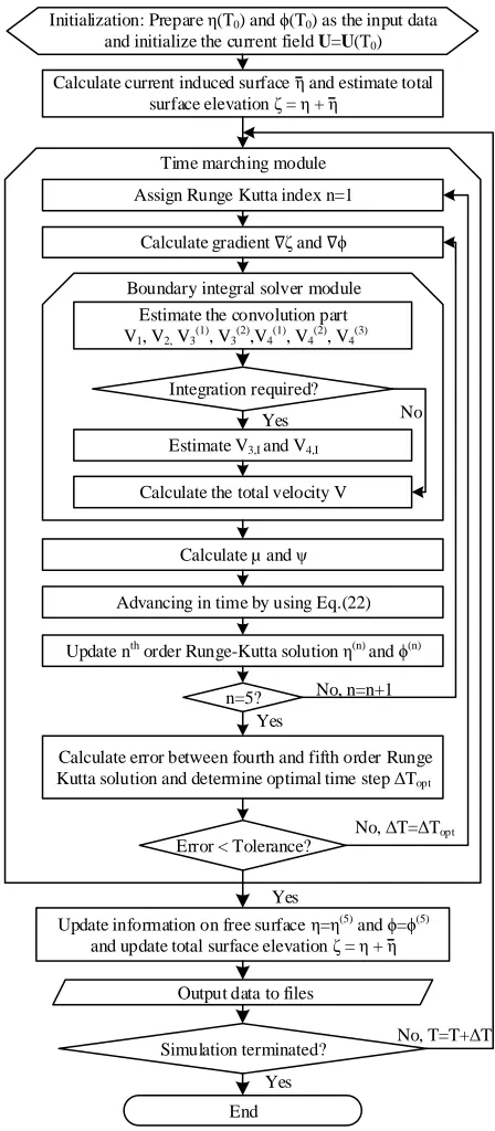
Based on the techniques introduced in section 2.2.1-2.2.3, a flow chart illustrating the numerical

Time marching module

Boundary integral solver module

Initialization: Prepare η(T0) and ϕ(T0) as the input data

and initialize the current field U=U(T0)

Simulation terminated? Output data to files Estimate the convolution part V1, V2, V3(1), V3(2),V4(1), V4(2), V4(3)

Integration required? Assign Runge Kutta index n=1

Error < Tolerance?

No, ΔT=ΔTopt

End Yes

Yes

Yes

No, T=T+ΔT Calculate gradient ζ and ϕ

No

Update information on free surface η=η(5) and ϕ=ϕ(5) and update total surface elevation ζ = η + η

Estimate V3,I and V4,I

Calculate the total velocity V

Calculate error between fourth and fifth order Runge Kutta solution and determine optimal time step ΔTopt

Calculate current induced surface η and estimate total surface elevation ζ = η + η

Update nth _{order Runge-Kutta solution η}(n) _{and ϕ}(n)

n=5? No, n=n+1

Yes Calculate µ and ψ

Advancing in time by using Eq.(22)

3

Validations

In order to demonstrate the effectiveness of the improved ESBI method for modelling the wave-current

interactions, some numerical simulations are performed in this section and the obtained results are

compared with the data in relevant literature.

3.1

Uniform current

Since a regular wave train on uniform current behaves similarly to that on spatially-varying current, the

case for it will be demonstrated in the section 3.2. Here firstly, a focusing wave on the uniform current is

simulated. The results are compared with the laboratory measurements in Wu & Yao [60], in which the

focusing wave is generated by using the formula

𝜂_𝑅 = ∑ 𝑎_𝑛cos(𝑘_𝑛𝑋 − 𝜔_𝑛𝑇 + 𝜃_𝑛)

𝑁

𝑛=1

(35)

where 𝑎𝑛, 𝑘𝑛 and 𝜔𝑛 are the amplitude, wave number and frequency of each individual component, 𝜃𝑛=

−𝑘𝑛𝑋𝑓+ 𝜔𝑛𝑇𝑓, 𝑋𝑓 and 𝑇𝑓 are specified focusing location and time respectively.

The computational domain covers 32 peak wave lengths, and is resolved into 1024 points. A pneumatic

wave maker is placed in the centre of the tank and the generated waves propagate towards both ends where

they are absorbed. The information of the components, such as 𝑎𝑛, 𝑘𝑛 and 𝜔𝑛, etc., are extracted from the

time history of the free surface in absence of the current in the literature. They are adjusted through

iterations to minimize the error of the present model for reproducing the same focusing wave measured in

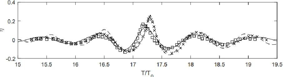
laboratory. Next, with the calibrated components, two cases with following and opposing current are

performed, where the velocity is ±0.1m/s. The time histories obtained by using the ESBI recorded at the

focusing location, in comparison with the one observed in laboratory, are displayed in Figure 2. It shows

that due to the wave-current interactions, the release of the wave packet on the following current was lagged,

while this feature was reversed on the opposing current. Nevertheless, the results obtained by using the

ESBI agree quite well with that recorded in the laboratory by Wu & Yao [60], where the errors of the

maximum crest are 7% and 10% for following and opposing current, respectively, which indicates that the

Figure 2. Comparison of the time history of free surface: rogue wave on uniform current. ’- - -’: ESBI,

U = 0.1m/s; ’x’: Wu and Yao [60], U = 0.1m/s; ’-’: ESBI, U = -0.1m/s; ’ ’: Wu and Yao [60], U = -0.1m/s

3.2

Two-dimensional spatially-varying current

In this subsection, the newly developed ESBI is employed to simulate two-dimensional uniform waves

propagating on spatially-varying current. The obtained results are then compared with those by using HOS

and those observed in laboratory to further validate the method.

3.2.1

Regular waves on collinear current

The numerical simulations by using HOS in Wu [50] are performed here by using the newly developed

ESBI model. The domain covers 256 wave lengths and 8192 points are used. The current profile is given

by

𝑼(𝑋, 𝑌) =

{

0,

𝑈𝑚𝐻((96𝐿0− 𝑋)/72𝐿0),

𝑈_𝑚,

𝑈𝑚𝐻((𝑋 − 160𝐿0)/72𝐿0),

0,

0 ≤ 𝑋 ≤ 24𝐿₀ 24𝐿₀< 𝑋 ≤ 96𝐿₀ 96𝐿₀< 𝑋 ≤ 160𝐿₀ 160𝐿₀< 𝑋 ≤ 232𝐿₀ 232𝐿₀< 𝑋 ≤ 256𝐿₀

(36)

and 𝐻( ) is the Hermitian polynomial,

𝐻(𝜉) = 1 − 462𝜉6_{+ 1980𝜉}7_{− 3465𝜉}8_{+ 3080𝜉}9_{− 1386𝜉}10_{+ 252𝜉}11 ₍₃₇₎

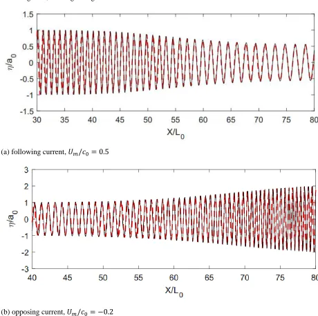
Both cases of following and opposing currents are considered, i.e., 𝑈𝑚/𝑐0 = 0.5 and 𝑈𝑚/𝑐0= −0.2,

where 𝑐0 is the wave phase speed. The computational domain is initialized by a spatially-periodical Stokes

wave train with steepness of 0.001 for linear waves and 0.2 for nonlinear waves, with simultaneous presence

of current. Due to the current effects, the local wave steepness will be changed gradually with time, and it

subjected to opposing current, wave breaking is observed due to the amplification effects induced by the

opposing current. Thus, the initial steepness is adjusted to 0.05 to avoid the wave breaking. The stabilized

free surface at the end of the simulation, in comparison with the surface elevation extracted from [50] is

shown in Figure 3, where good agreement is observed.

(a) following current, 𝑈𝑚/𝑐0= 0.5

(b) opposing current, 𝑈_𝑚/𝑐₀ = −0.2

Figure 3. Comparison of the free surface in space: regular waves of steepness 0.001 on collinear

current. ’- - -’: Numerical results in [50]; ’-’: Results by ESBI

To further demonstrate the effectiveness of the ESBI for this case, the local wave amplitude and wave

𝑎_𝑙 = √𝜂2_{+ 𝜂}

𝐻2 𝑎𝑛𝑑 𝑘𝑙 =

𝜂𝜕_𝑇𝜂_𝐻− 𝜂_𝐻𝜕_𝑇𝜂 𝜂2_{+ 𝜂}

𝐻

2 (38)

where 𝜂𝐻 stands for the corresponding Hilbert transform of the free surface elevation. Then the relationship

between the local wave steepness against the current velocity, in comparison with the linear analytical

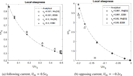
solution and the results in Wu [50] is presented in Figure 4.

The figure shows that when the wave steepness is small, both the numerical results obtained by using

the ESBI and HOS agree with the linear predictions. However, the results deviate from the linear theory

when wave steepness becomes large, which is understandable as the contribution from the nonlinearities

becomes significant. Both HOS and ESBI overpredict the steepness in following current while

underestimate that in opposing current. However, the maximum differences between the obtained results

by using the ESBI and HOS are about 4.6% and 4.1% for the following and opposing current, respectively,

and the ESBI model slightly overpredicts the wave steepness when the flow is relatively faster. As indicated

in section 2.1, the HOS suggested by Wu [50] is only accurate for modelling current interacting with small

steepness waves. Therefore, the difference between the results of the two approaches is due to that the HOS

had neglected higher order nonlinear terms representing the wave-current interactions. The neglected terms

will become pronounced when the wave steepness increases, in which cases the HOS becomes less accurate.

Nevertheless, the good agreement between the ESBI and theoretical results is observed.

(a) following current, 𝑈𝑚= 0.5𝑐0 (b) opposing current, 𝑈𝑚 = −0.2𝑐0

3.2.2

Wave blocking on opposing current

Waves propagating against an opposing current may be blocked at a certain point if the current is

sufficiently strong. To validate the ESBI for simulating such situations, three cases subject to horizontally

shearing current studied by Ma, et al. [61] in laboratory are selected. The cases have a variety of nonlinear

scenarios. The configuration of the numerical wave tank is the same as that in section 3.1, however, the

pneumatic wave maker is moved to one fourth of the tank length from the left boundary, and only the part

on the right is effectively used for simulating the wave propagation in the cases.

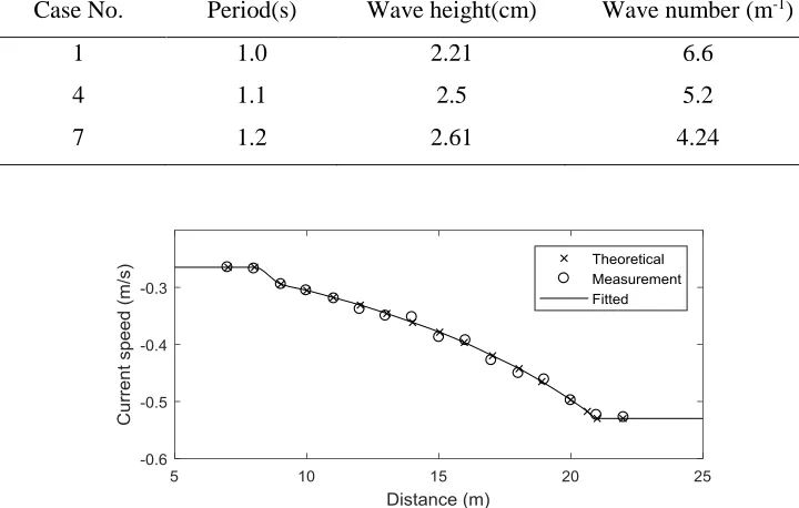
The profile of the current is obtained by interpolating the measured velocity in laboratory, as shown by

the ‘Fitted’ data in Figure 5, which is then prescribed to be 𝑼 in the ESBI simulation. The wave conditions

of the selected cases are given in Table 1, where the maximum wave steepness is 0.073 (Case 1). Each

simulation lasts for 400 periods, and the last 100 periods are extracted for spectral analysis by using the

Fourier transform. By doing so, the local frequency (𝜔𝑙) corresponding to the peak of the obtained spectra

at all probes along the tank can be estimated and the results are shown in Figure 6.

Table 1. Description of the configuration

Case No. Period(s) Wave height(cm) Wave number (m-1₎

1 1.0 2.21 6.6

4 1.1 2.5 5.2

7 1.2 2.61 4.24

Figure 5. Profile of horizontally shearing current against distance: wave blocking on opposing

(a) Case 1 (b) Case 4

(c) Case 7

Figure 6. Local wave frequency against distance. ‘−’: ESBI; ‘•’ Measurements by Ma, et al. [61]

It can be found that in the first two cases, i.e., Case 1&4, the waves are relatively short and the phase

celerity is not fast enough to compete with the current speed. Therefore, the waves are blocked at certain

points. Instant frequency down-shifting is observed. For the last case, i.e., Case 7, the waves are moving

sufficiently fast to penetrate the current field, despite of slight frequency down-shifting near the end of the

tank. Moreover, the numerical results obtained by using the ESBI are well consistent with these measured

in the laboratory. In particular, the ESBI model successfully captured the frequency down-shifting due to

the blocking effects of the opposing current observed in laboratory.

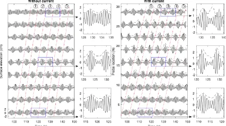
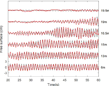
In addition, the comparison of the free surface time history between the laboratory experimental data

and numerical simulation results recorded at the gauges along the tank for case 1 is shown in Figure 7. It is

understandable that the envelope represents the evolution of the wave energy along the tank, so that can be

used to indicate the blocking effects of the current on the propagation of the waves. The figure shows that

the free surface time histories predicted by the ESBI agree reasonably with the experimental data, though

the measured free surface in laboratory behaves irregularly, which may be caused by the imperfection for

reproducing steady current condition, e.g., the turbulence of the current as observed [61]. However, the

Figure 7. Comparison of the time histories of the surface elevation for case 1 of wave steepness

0.073. ‘−’: free surface by ESBI, ‘· · ·’: laboratory measurement in [61].

3.3

Three-dimensional Horizontally-shearing current

In addition to the two-dimensional validation cases, three-dimensional simulations are also performed

to demonstrate the robustness and effectiveness of the newly developed ESBI method, for modelling waves

interacting with horizontally-shearing current. Waves propagating on an oblique current is more

complicated. It was firstly studied by Shyu and Tung [10] by using the ray theory. Subsequently, Lavrenov

[3] analyzed the ray pattern of the Agulhas current and found that the rogue waves can be generated at the

focusing point where wave energy concentrates. Later studies pointed out that wave-current interaction is

the major mechanism of the rogue wave phenomenon in deep water [9, 62]. Hereafter, two cases are

considered, i.e., the modulation instability induced by oblique opposing current, and the spreading seas

entering a horizontally-shearing current field. The simulations of the selected two cases have been

performed in a physical wave tank by Toffoli, et al. [63]. These cases will be reproduced by using the ESBI

3.3.1

Modulation instability

The NWT covers 78m×58m in space and is resolved into 2048×512 collocation pointes, whilst the

directional wave maker is installed at one fourth of the total length from the left boundary. Waves are

absorbed at far ends and only the part on the right of the wave maker is effectively used. Three components

are input to generate the wave maker signal, where the steepness of the main wave (carrier wave) is 0.1 and

period 0.8s, including two side-bands with 1/4 the amplitude of carrier wave and bandwidth equals to 0.25.

The current flows obliquely in an angle of Ψ = 110𝑜 with respect to the main wave direction. The configuration of the NWT is shown in Figure 8. The maximum current speed is 0.2m/s near the centre of

the wave tank, however, exact values of the current speed is unavailable except the measurements at five

individual current meters. To initialize the current field in the ESBI, the current profile is approximated by

using

|𝑼| =

{

−0.104,

−0.104 − 0.027 × 𝐻((12 − 𝑋/𝐿0)/7),

−0.131,

−0.104 − 0.027 × 𝐻((𝑋/𝐿0− 17)/7),

−0.104,

𝑋/𝐿0≤ 5

5 < 𝑋/𝐿₀≤ 12 12 < 𝑋/𝐿₀≤ 17 17 < 𝑋/𝐿0≤ 24

𝑋/𝐿0 > 24

(39)

It is found the fitted results agree very well with the measurement in Toffoli, et al. [63], as shown in Figure

9, where the maximum error is about 2.0%.

Figure 9. Fitted profile of the current speed. ’x’: Measured in Toffoli, et al.[63]; ’—’: Fitted.

The three-dimensional free surface distributions in space at the end of the simulation are shown in Figure

10 for the cases with and without the current. It can be found in Figure 10 (a) that around 11.5 wave groups

coexist in the computational domain when current is not present. However, as shown in Figure 10 (b), due

to the current effects, the waves are compressed and 13 groups are observed in the NWT simultaneously.

Meanwhile, the wave heights are found larger than those in absence of current. In addition, during the

simulation, the data of the free surface elevation are collected at 9 wave gauges along the main wave

direction, and the comparison of the time histories of the free surface elevation between the numerical

results and that reported in Toffoli, et al. [63] is shown in Figure 11. It is found that without the current,

since the wave train features a small Benjamin-Feir Index, the modulation instability cannot develop into

extreme waves during the propagation. Whereas the waves are compressed due to the presence of opposing

current, which increases the Benjamin-Feir Index, thus the instability is triggered and the maximum free

surface is achieved around gauge #5 and #6. Meanwhile, the ESBI successfully captured the variation of

the surface elevation at different locations and the results agree quite well with the laboratory experiment

in both the cases with and without current. However, it should be noted that in the case with current, the

time series measured in physical tank are more erratic than the ones in NWT, which is presumably related

to the turbulence fluctuation of the current velocity [63]. Nevertheless, the evolution of the wave packet

predicted by the numerical results is qualitatively consistent with the laboratory observations.

(b) with current

Figure 10. The spatial distribution of modulated free surface at T/T0 = 150 (Color online)

Figure 11. Comparison of the time histories of the surface elevation. ‘-’: free surface by ESBI,

‘- -’: surface envelope in Toffoli, et al. [63] (Color online).

To further demonstrate the robustness of the ESBI quantitively, the propagation of 5 individual wave

groups are tracked, as shown in Figure 11 between the dash lines. Their maximum crests recorded at each

probe are extracted, which are then normalized by the concurrent variances and shown in Figure 12. To

remove the erratic feature of the data collected in the laboratory, the mean value is estimated by averaging

the values indicated by the 5 curves, and is also displayed in the figure. Meanwhile, the numerical data is

identical among each individual wave group, thus only the mean value is displayed and compared with that

well with that in Toffoli, et al. [63], where the maximum error between the numerical results and the mean

value of laboratory observation in presence of current is about 9.8% at gauge #5. The good agreement

reveals that the present ESBI model successfully captured the dynamics of the unstable wave train.

Figure 12. Comparison of the maximum free surface against location. ’· · ◦ · ·’: Group (1) in

[63]; ‘· · Δ · ·’: Group (2) in [63]; ‘· · □ · ·’: Group (3) in [63]; ‘··+··’: Group (4) in [63]; ‘· · × · ·’: Group (5) in [63]; ‘- - -’: Average in [63]; ‘—’: ESBI.

3.3.2

Spreading seas

To show that the present model is not limited to only model regular waves in three dimensions, it is

then verified for simulating spreading seas with presence of horizontally shearing current. The

configuration of the NWT is the same with that in section 3.3.1, and the JONSWAP spectrum is employed,

where the peak period is 1s, significant wave height 0.08m and peak enhancement factor 6. The spreading

function is chosen as

𝐺(𝜃) = Γ(𝑁/2 + 1) √𝜋Γ[(𝑁 + 1)/2]cos

𝑁_{(𝜃) (40)}

where Γ() is the Gamma function and N = 24. The mean wave direction, the current velocity and direction are both the same with that in section 3.3.1.

Snapshots of the free surface elevation in space at T/T0 = 150 are presented in Figure 13, in which a

qualitative comparison between Figure 13(a) and (b) reveals that the number of extreme waves in presence

of current are more than that without current presence. This is understandable as the opposing current can

contribute to the probability of extreme wave events [1]. To examine the accuracy of the numerical model

surface is unavailable and direct comparison of the surface elevation cannot be made, only the kurtosis at

different locations along the main wave direction is analyzed. It is estimated by using the formula

𝜅4= 𝑚4/𝑚22 (41)

where 𝑚4 and 𝑚2 are the fourth and second moment of the surface time history, respectively. In fact, the

kurtosis reflects the probability of the extreme waves in random wave field [1], thus is sufficient to examine

the enhancement of the nonlinearities of the wave field due to the current. Based on the linear theory, when

the wave steepness is small, the statistics of the random sea follows the Gaussian distribution, which makes

kurtosis identical to 3. However, when the wave steepness increases, the nonlinearities become stronger

and the kurtosis will exceed 3. To approximate the kurtosis while considering nonlinear effects up to the

second order, a formula is suggested by Longuet-Higgins [64] as below

𝜅₄′ _{= 3 + 24𝜎}2 ₍₄₂₎

and 𝜎 is the standard deviation of the surface elevation.

The results obtained by using the numerical simulation, together with that estimated by using Eq. (42)

and obtained in the physical wave tank [63] are presented in Figure 14. It shows good agreement between

the curves obtained numerically and experimentally. Moreover, it is observed that the kurtosis is subjected

to a deceleration of its growth throughout the propagation, meanwhile, shows the tendency to preserve

slightly higher values with current presence. At the far end from the wave maker, the kurtosis agrees very

well with the second order prediction without the current, whereas it is significanly underestimated when

current is involved. In the middle part o the tank, the resutls of Eq. (42) is close to the expeimental data of

the cases with current. However, the difference betwwen the values of the kurtosis with and witout the

current is successfully captured by the numerical simulation. These results desmonstrated that Eq. (42)

may not correctly reflect the evolution of the kurtosis throughout the whole tank. In addition, the errors of

the maximum kurtosis between the results obtained in the NWT and physcial wave tanks are 0.8% and 1.7%

corresponding to the cases without and with current, respectively. These indicates that the present ESBI

(a) without current

(b) with current

Figure 13. The spatial distribution of spreading wave free surface at T/T0 = 150 (Color online)

’—◦—’: without current, Toffoli, et al.[63]; ’—•—’: with current, Toffoli, et al. [63]; ’—Δ—’: without current, ESBI; ’—▲—’: with current, ESBI.

4

Conclusion

This study suggests an accurate and efficient phase-resolved numerical method to model the fully

nonlinear three-dimensional interactions between waves and horizontally varying current. To achieve this

goal, a new system of equations describing the fully nonlinear interactions between waves and varying

current is proposed, removing the limitation to the small wave steepness of the existing formulation in

literature. The Enhanced Spectral Boundary Integral (ESBI) Method is extended to solve the problems

based on the new equations by considering the extra terms associated with wave-current interaction. The

newly developed method can be employed to simulate the real evolution of ocean waves on current, which

may not be done correctly by the existing methods in literature.

The newly developed method based on the new equations is compared with experimental data available

in literature in the several cases, including dimensional focusing waves on an uniform current,

two-dimensional regular waves interacting with spatially-varying current and three-two-dimensional interaction of

horizontal varying current with spreading ocean waves and modulated waves generated by superposing

two-sideband wave components onto a carrier wave component. It is found in two dimensions that the

release of the focusing wave packet on the following uniform current was lagged, while it was reversed on

the opposing uniform current. When waves were subjected to horizontally shearing current, instant

frequency down-shifting of the wave train along the tank was observed, due to the blockage of the opposing

current. In addition, when waves propagated opposed to oblique horizontally shearing current in three

dimensions, modulated uniform wave train featuring small Benjamin-Feir index could develop into large

steepness waves due to modulation instability. Apart from these, the kurtosis of the spreading random sea

was shown to preserve slightly higher values with current presence. It is also found that generally good

agreement between the numerical results from the newly developed method and laboratory measurements

is achieved in all the cases considered. This indicates that the method works well when it is employed to

model the two or three dimensional, fully nonlinear wave-current interactions in the cases with uniform or

horizontally sheared current. Furthermore, the phase of each individual wave is resolved, so that not only

the statistical information, but also the kinematics and dynamics of the fully nonlinear wave-current field

can be obtained, which are of great importance for the sake of engineering purposes.

As demonstrated in section 3.2.1, the some differences between the results obtained with the HOS and

attributed to the nature of the HOS approach, i.e., the formulations suggested by Dommermuth and Yue

[65] as those employed by Wu [50]. On one hand, the HOS model did not account for higher order nonlinear

terms representing wave-current interactions. On the other hand, it fails to preserve the Hamiltonian

structure of the prognostic equations[66], of which the insufficiency is reported for modeling long-time

wave propagation [67]. Although it can be improved by employing another version of the HOS suggested

by West, et al. [68], further investigations are required.

Nevertheless, the limitation of the present model is that it can only be used to model non-breaking waves,

as the methodology itself is based on the potential theory that assumes the water is inviscid and irrotational.

In the future study, the present model will be coupled with other methods which can deal with the breaking

waves to overcome the drawback. Moreover, the present model may be insufficient for modeling waves

subject to strong vertically shearing current, which is important for studying waves near shore and in coastal

areas. In the future, the present ESBI model will be extended to include this feature, based perhaps on the

work by Fructus and Grue [69], in which variable bathymetry is considered.

Acknowledgements

The authors gratefully acknowledge the financial support of EPSRC, UK (EP/N006569/1,

EP/N008863/1 and EP/M022382/1) and DST-UKIERI project (DST-UKIERI-2016-17-0029). The authors

also appreciate Dr. Yuxiang Ma for providing the experimental data.

Appendix

The formulas for estimating 𝑉3 and 𝑉4 are presented here without further details but can be found in [55],

where the convolution part of 𝑉3 is given by

𝐹 {𝑉₃(1)} = −𝐾

6[𝐾𝑖𝑲 ∙ 𝐹{𝜁3∇𝜙̃} − 3𝐹 {𝜁𝐹−1{𝐾𝑖𝑲 ∙ 𝐹{𝜁2∇𝜙̃}}}

+ 3𝐹 {𝜁2_𝐹−1_{{𝐾𝑖𝑲 ∙ 𝐹{𝜁∇𝜙̃}}} + 𝐹 {𝜁}3_𝐹−1_{𝐾3_{𝐹{𝜙̃}}}]}

𝐹 {𝑉₃(2)} = − 𝐾

120[𝑖𝑲𝐾3∙ 𝐹{𝜁5∇𝜙̃} − 5𝐹 {𝜁𝐹−1{𝑖𝑲𝐾3∙ 𝐹{𝜁4∇𝜙̃}}} + 10𝐹 {𝜁2_𝐹−1_{{𝑖𝑲𝐾}3_{∙ 𝐹{𝜁}3_∇𝜙̃}}}

− 10𝐹 {𝜁3_𝐹−1_{{𝑖𝑲𝐾}3_{∙ 𝐹{𝜁}2_∇𝜙̃}}}

+ 5𝐹 {𝜁4_𝐹−1_{{𝑖𝑲𝐾}3_{∙ 𝐹{𝜁∇𝜙̃}}} + 𝐹 {𝜁}5_𝐹−1_{𝐾5_{𝐹{𝜙̃}}}]}

(A. 2)

and the integration part

𝐹{𝑉3,𝐼} =

𝐾 2𝜋𝐹 {

35

16∫ 𝜙̃′∇′∙ [(𝜁′− 𝜁)∇′ 1

𝑅] 𝐷6𝑑𝑿′ + ∫ 𝜙̃′_{[1 − (1 + 𝐷}2₎−3/2₋3

2𝐷2+ 15

8 𝐷4− 35 16𝐷6] ∇′ ∙ [(𝜁′_{− 𝜁)∇}′1

𝑅] 𝑑𝑿′}

(A. 3)

Meanwhile, the convolution part 𝑉4 is given by

𝐹 {𝑉₄(1)} = −𝐾

2[𝐾𝐹{𝜁2𝑉} − 2𝐹 {𝜁𝐹−1{𝐾𝐹{𝜁𝑉}}} + 𝐹 {𝜁2𝐹−1{𝐾𝐹{𝑉}}}] (A. 4) 𝐹 {𝑉₄(2)} = − 𝐾

24[𝐾3𝐹{𝑉𝜁4} − 4𝐹 {𝜁𝐹−1{𝐾3𝐹{𝑉𝜁3}}} + 6𝐹 {𝜁2𝐹−1{𝐾3𝐹{𝑉𝜁2}}} − 4𝐹 {𝜁3_𝐹−1_{𝐾3_{𝐹{𝑉𝜁}}} + 𝐹 {𝜁}4_𝐹−1_{𝐾3_{𝐹{𝑉}}}]}

(A. 5)

𝐹 {𝑉₄(3)} =−𝐾

720[𝐾5𝐹{𝑉𝜁6} − 6𝐹 {𝜁𝐹−1{𝐾5𝐹{𝑉𝜁5}}}

+ 15𝐹 {𝜁2_𝐹−1_{𝐾5_{𝐹{𝑉𝜁}4_{}}} − 20𝐹 {𝜁}3_𝐹−1_{𝐾5_{𝐹{𝑉𝜁}3_}}}

+ 15𝐹 {𝜁4_𝐹−1_{𝐾5_{𝐹{𝑉𝜁}2_{}}} − 6𝐹 {𝜁}5_𝐹−1_{𝐾5_{𝐹{𝑉𝜁}}}}

+ 𝐹 {𝜁6_𝐹−1_{𝐾5_{𝐹{𝑉}}}]}

(A. 6)

and the integration part

𝐹{𝑉4,𝐼} =

𝐾 2𝜋𝐹 {∫

𝑉′

𝑅(1 − 1 √1 + 𝐷2−

1 2𝐷2+

3 8𝐷4−

5

16𝐷6) 𝑑𝑿′} (A. 7)

References

Springer-Verlag, 2009.

[2] M. Gerber, The interaction of deep-water gravity waves and an annular current: linear theory,

Journal of Fluid Mechanics. 248 (1993) 153-172.

[3] I. V. Lavrenov, The wave energy concentration at the Agulhas current off South Africa,

Natural Hazards. 17 (2) (1998) 117-127.

[4] I. V. Lavrenov and A. V. Porubov, Three reasons for freak wave generation in the

non-uniform current, European Journal of Mechanics-B/Fluids. 25 (5) (2006) 574-585.

[5] D. H. Peregrine, Interaction of water waves and currents, Advances in Applied Mechanics.

16 (1976) 9-117.

[6] G. P. Thomas, Wave-current interactions: an experimental and numerical study. Part 1. Linear

waves, Journal of Fluid Mechanics. 110 (1981) 457-474.

[7] G. P. Thomas, Wave-current interactions: an experimental and numerical study. Part 2.

Nonlinear waves, Journal of Fluid Mechanics. 216 (1990) 505-536.

[8] J. H. Shyu and O. M. Phillips, The blockage of gravity and capillary waves by longer waves

and currents, Journal of Fluid Mechanics. 217 (1990) 115-141.

[9] B. S. White and B. Fornberg, On the chance of freak waves at sea, Journal of Fluid

Mechanics. 355 (1998) 113-138.

[10] J. H. Shyu and C. C. Tung, Reflection of oblique waves by currents: analytical solutions and

their application to numerical computations, Journal of Fluid Mechanics. 396 (1999)

143-182.

[11] I. G. Jonsson, C. Skougaard and J. D. Wang, Interaction between waves and currents, Coastal

Engineering. (1970) 489-507.

[12] I. G. Jonsson, Wave-current interactions, Ocean Engineering Science: The Sea. 9 (A) (1990)

65-120.

[13] S. B. Yoon and P. L. F. Liu, Interactions of currents and weakly nonlinear water waves in

shallow water, Journal of fluid mechanics. 205 (1989) 397-419.

[14] Q. Chen, P. A. Madsen, H. A. Schäffer and D. R. Basco, Wave-current interaction based on

an enhanced Boussinesq approach, Coastal Engineering. 33 (1) (1998) 11-39.

the elliptic mild-slope wave equation, Ocean Engineering. 32 (17) (2005) 2135-2164.

[16] M. F. Gobbi, J. T. Kirby and G. E. Wei, A fully nonlinear Boussinesq model for surface

waves. Part 2. Extension to O (kh) 4, Journal of Fluid Mechanics. 405 (2000) 181-210.

[17] P. J. Lynett, A multi-layer approach to modeling generation, propagation, and interaction of

water waves (PhD thesis), New York: Cornell University, 2002.

[18] M. Isaacson and K. F. Cheung, Time-domain solution for wave—current interactions with a

two-dimensional body, Applied Ocean Research. 15 (1) (1993) 39-52.

[19] D. J. Kim and M. H. Kim, Wave-Current-Body Interaction by a Tune-D0main High-Order

Boundary Element Method. Honolulu, 1997.

[20] P. Ferrant, Runup on a cylinder due to waves and current: potential flow solution with fully

nonlinear boundary conditions, International Journal of Offshore and Polar Engineering. 11

(1) (2001) 1-9.

[21] S. Ryu, M. H. Kim and P. J. Lynett, Fully nonlinear wave-current interactions and kinematics

by a BEM-based numerical wave tank, Computational Mechanics. 32 (4-6) (2003) 336-346.

[22] R. M. Moreira and D. H. Peregrine, Nonlinear interactions between deep-water waves and

currents, Journal of Fluid Mechanics. 691 (2012) 1-25.

[23] S. Yan, Q. W. Ma and T. A. A. Adcock, Investigations of freak waves on uniform current,

Harbin, 2010.

[24] D. G. Dommermuth and D. K. Yue, The nonlinear three-dimensional waves generated by a

moving surface disturbance. Hague, Netherlands, 1988.

[25] J. Grue and A. Jensen, Orbital velocity and breaking in steep random gravity waves, Journal

of Geophysical Research: Oceans. 117 (C7) (2012) 0148-0227.

[26] J. C. Park, M. H. Kim and H. Miyata, Three-dimensional numerical wave tank simulations

on fully nonlinear wave–current–body interactions, Journal of Marine Science and

Technology. 6 (2) (2001) 70-82.

[27] H. C. Chen and K. Yu, CFD simulations of wave–current-body interactions including

greenwater and wet deck slamming, Computers & Fluids. 38 (5) (2009) 970-980.

[29] F. P. Bretherton and C. J. Garrett, Wavetrains in inhomogeneous moving media, Proceedings

of the Royal Society of London A: Mathematical, Physical and Engineering Sciences. 302

(1471) (1968) 529-554.

[30] R. A. Dalrymple, A finite amplitude wave on a linear shear current, Journal of Geophysical

Research. 79 (30) (1974) 4498-4504.

[31] J. A. Simmen and P. G. Saffman, Steady Deep‐Water Waves on a Linear Shear Current,

Studies in Applied Mathematics. 73 (1) (1985) 35-57.

[32] A. T. Da Silva and D. H. Peregrine, Steep, steady surface waves on water of finite depth with

constant vorticity, Journal of Fluid Mechanics. 195 (1988) 281-302.

[33] N. Kishida and R. J. Sobey, Stokes theory for waves on linear shear current, Journal of

Engineering Mechanics. 114 (8) (1988) 1317-1334.

[34] A. Constantin and W. Strauss, Exact steady periodic water waves with vorticity,

Communications on Pure and Applied Mathematics. 57 (4) (2004) 481-527.

[35] O. S. Pak and K. W. Chow, Free surface waves on shear currents with non-uniform vorticity:

third-order solutions, Fluid Dynamics Research. 41 (3) (2009) 035511.

[36] W. Choi, Nonlinear surface waves interacting with a linear shear current, Mathematics and

Computers in Simulation. 80 (1) (2009) 29-36.

[37] O. G. Nwogu, Interaction of finite-amplitude waves with vertically sheared current fields,

Journal of Fluid Mechanics. 627 (2009) 179-213.

[38] A. Constantin and E. Varvaruca, Steady periodic water waves with constant vorticity:

regularity and local bifurcation, Archive for Rational Mechanics and Analysis. 199 (1) (2011)

33-67.

[39] V. Kozlov and N. Kuznetsov, Dispersion equation for water waves with vorticity and Stokes

waves on flows with counter-currents, Archive for Rational Mechanics and Analysis. 214 (3)

(2014) 971-1018.

[40] R. Ribeiro, P. A. Milewski and A. Nachbin, Flow structure beneath rotational water waves

with stagnation points, Journal of Fluid Mechanics. 812 (2017) 792-814.

659.

[42] H. Tamura, T. Waseda, Y. Miyazawa and K. Komatsu, Current-induced modulation of the

ocean wave spectrum and the role of nonlinear energy transfer, Journal of Physical

Oceanography. 38 (12) (2008) 2662-2684.

[43] F. M. Turpin, C. Benmoussa and C. C. Mei, Effects of slowly varying depth and current on

the evolution of a Stokes wavepacket, Journal of Fluid Mechanics. 132 (1983) 1-23.

[44] M. Gerber, The Benjamin-Feir instability of a deep-water Stokes wavepacket in the presence

of a non-uniform medium, Journal of Fluid Mechanics. 176 (1987) 311-332.

[45] A. V. D. Cornelis, The effect of non-uniformity of modulated wavepackets on the mechanism

of benjamin-feir instability, Journal of Fluid Mechanics. 399 (1999) 237-249.

[46] T. T. Janssen and T. H. C. Herbers, Nonlinear wave statistics in a focal zone, Journal of

Physical Oceanography. 39 (8) (2009) 1948-1964.

[47] K. B. Hjelmervik and K. Trulsen, Freak wave statistics on collinear currents, Journal of Fluid

Mechanics. 637 (2009) 267-284.

[48] J. R. Stocker and D. H. Peregrine, The current-modified nonlinear Schrödinger equation,

Journal of Fluid Mechanics. 399 (1999) 335-353.

[49] J. Wang, Q. Ma and S. Yan, On quantitative errors of two simplified unsteady models for

simulating unidirectional nonlinear random waves on large scale in deep sea, Physics of

Fluids. 29 (6) (2017) 067107.

[50] G. Wu, Direct Simulation and Deterministic Prediction of Large-scale Nonlinear Ocean

Wave-field (PhD Thesis), Massachusetts, USA: Massachusetts Institute of Technology,

2004.

[51] D. Clamond and J. Grue, A fast method for fully nonlinear water-wave computations, Journal

of Fluid Mechanics. 447 (2001) 337-355.

[52] D. Fructus, D. Clamond, J. Grue and O. Kristiansen, An efficient model for

three-dimensional surface wave simulations Part I: Free space problems, Journal of Computational

Physics. 205 (2005) 665-685.

Computational Physics. 205 (2005) 686-705.

[54] J. Grue, Computation formulas by FFT of the nonlinear orbital velocity in three-dimensional

surface wave fields, J. Eng. Math. 67 (2010) 55-69.

[55] J. Wang and Q. W. Ma, Numerical techniques on improving computational efficiency of

Spectral Boundary Integral Method, International Journal for Numerical Methods in

Engineering. 102 (10) (2015) 1638-1669.

[56] D. Fructus, C. Kharif, M. Francius, Ø. Kristiansen, D. Clamond and J. Grue, Dynamics of

crescent water wave patterns, Journal of Fluid Mechanics. 537 (2005) 155-186.

[57] P. P. Sullivan and J. C. McWilliams, Dynamics of winds and currents coupled to surface

waves, Annual Review of Fluid Mechanics. 42 (2010) 19-42.

[58] J. Grue and J. Kolaas, Experimental particle paths and drift velocity in steep waves at finite

water depth, Journal of Fluid Mechanics. 810 (2017) R1.

[59] J. Wang and Q. W. Ma, Numerical Investigation on Limitation of Boussinesq Equation for

Generating Focusing Waves, Procedia Engineering. 126 (2015) 597-601.

[60] C. H. Wu and A. Yao, Laboratory measurements of limiting freak waves on currents, Journal

of Geophysical Research: Oceans. 109 (2004) C12002.

[61] Y. Ma, G. Dong, M. Perlin, X. Ma, G. Wang and J. Xu, Laboratory observations of wave

evolution, modulation and blocking due to spatially varying opposing currents, Journal of

Fluid Mechanics. 661 (2010) 108-129.

[62] A. Toffoli, J. M. Lefevre, E. Bitner-Gregersen and J. Monbaliu, Towards the identification

of warning criteria: analysis of a ship accident database, Applied Ocean Research. 27(6)

(2005) 281-291.

[63] A. Toffoli, L. Cavaleri, A. Babanin, M. Benoit, E. Bitner-Gregersen, J. Monbaliu, M.

Onorato, A. Osborne and C. Stansberg, Occurrence of extreme waves in three-dimensional

mechanically generated wave fields propagating over an oblique current, Natural Hazards

and Earth System Sciences. 11 (3) (2011) 895-903.

[64] M. S. Longuet-Higgins, The effect of non-linearities on statistical distributions in the theory

of sea waves, Journal of Fluid Mechanics. 17 (3) (1963) 459-480.

gravity waves, Journal of Fluid Mechanics. 184 (1987) 267-288.

[66] J. Touboul and C. Kharif, Numerical simulations of water waves’ modulational instability

under the action of wind and dissipation, in: Numerical Simulation-From Theory to Industry,

InTech, 2012.

[67] D. Clamond, M. Francius, J. Grue and C. Kharif, Long time interaction of envelope solitons

and freak wave formations, European Journal of Mechanics-B/Fluids. 25 (5) (2006)

536-553.

[68] B. J. West, K. A. Brueckner, R. S. Janda, D. M. Milder, R. L. Milton, A new numerical

method for surface hydrodynamics, Journal of Geophysical Research: Oceans. 92 (C11)

(1987) 11803-11824.