White Rose Research Online URL for this paper:
http://eprints.whiterose.ac.uk/93025/
Version: Accepted Version
Article:
Mambrini, A. and Sudholt, D. (2015) Design and Analysis of Schemes for Adapting
Migration Intervals in Parallel Evolutionary Algorithms. Evolutionary Computation, 23 (4).
pp. 559-582. ISSN 1530-9304
https://doi.org/10.1162/EVCO_a_00153
[email protected] https://eprints.whiterose.ac.uk/
Reuse
Unless indicated otherwise, fulltext items are protected by copyright with all rights reserved. The copyright exception in section 29 of the Copyright, Designs and Patents Act 1988 allows the making of a single copy solely for the purpose of non-commercial research or private study within the limits of fair dealing. The publisher or other rights-holder may allow further reproduction and re-use of this version - refer to the White Rose Research Online record for this item. Where records identify the publisher as the copyright holder, users can verify any specific terms of use on the publisher’s website.
Takedown
If you consider content in White Rose Research Online to be in breach of UK law, please notify us by
Algorithms
Andrea Mambrini
School of Computer Science, University of Birmingham, Birmingham B15 2TT, United Kingdom
Dirk Sudholt
Department of Computer Science, University of Sheffield, Sheffield S1 4DP, United Kingdom
Abstract
The migration interval is one of the fundamental parameters governing the dynamic behaviour of island models. Yet, there is little understanding on how this parameter affects performance, and how to optimally set it given a problem in hand. We propose schemes for adapting the migration interval according to whether fitness improve-ments have been found. As long as no improvement is found, the migration interval is increased to minimise communication. Once the best fitness has improved, the mi-gration interval is decreased to spread new best solutions more quickly. We provide a method for obtaining upper bounds on the expected running time and the communi-cation effort, defined as the expected number of migrants sent. Example applicommuni-cations of this method to common example functions show that our adaptive schemes are able to compete with, or even outperform the optimal fixed choice of the migration interval, with regard to running time and communication effort.
Keywords
Parallel evolutionary algorithms, island model, migration interval, runtime analysis, theory
1
Introduction
Evolutionary algorithms (EAs) have given rise to many parallel variants [19, 28] fu-elled by the rapidly increasing number of CPU cores and the ready availability of computation power through GPUs and cloud computing. Parallelization provides a cost-effective approach to solving problems in real time and for tackling large-scale problems.
time. Everyτ generations, for some fixed parameterτ calledmigration interval, indi-viduals migrate between these islands to coordinate searches on the island. Communi-cation takes place according to a spatial structure, a topology connecting populations. Common topologies include rings, two-dimensional grids or toroids, hypercubes, or complete graphs with all possible connections.
Island models are popular optimisers for several reasons:
• Multiple communicating populations can make the same progress as a single pop-ulation in a fraction of the time, speeding up computation.
• Smaller populations can be simulated faster than large populations, effectively re-ducing the execution time on each processor [1].
• Periodic communication only requires small bandwidth if the migration interval is not very small, leading to low communication costs.
• Solution quality is improved as different populations can explore different regions of the search space.
The usefulness of parallel populations has been demonstrated in thousands of success-ful applications ranging from language tagging, circuit design, scheduling and plan-ning to bioinformatics [19, 3].
However, designing an effective parallel evolutionary algorithm can be challeng-ing as the method and amount of communication needs to be tuned carefully. Too frequent communication leads to high communication costs, and it can compromise exploration. Too little communication means that the populations become too isolated and unable to coordinate their searches effectively. There is agreement that even the ef-fect of the most fundamental parameters on performance is not well understood [19, 3].
We make a contribution towards finding good values for the migration interval, the parameter describing the frequency of migration. We propose adaptive schemes that adjust the migration interval, depending on whether islands have managed to find improvements during the last migration interval or not. The goal is to reduce communication, while not compromising the exploitation of good solutions. The main idea of our schemes is that if an island has managed to improve its current best fitness, migration should be intensified to spread this solution to other islands. Otherwise, islands decrease the frequency of migration in order to avoid large communication costs.
Two different adaptive schemes are proposed, inspired by previous work [11]. In both of them islands have individual migration intervals which are adapted through-out the run. In Scheme A if an island has not improved its current best fitness during the last migration interval, its migration interval is doubled. Once an improvement is found, the migration interval is set to 1 to communicate this new solution quickly. In Scheme B an island also doubles the migration interval when no improvement was found, while when an improvement is found, it halvesτ at the end of the current mi-gration interval.
We contribute a rigorous analytical framework that yields upper bounds on the expected optimisation time and the expected communication effort, defined as the to-tal number of migrants sent. This is done for fixed migration intervals in Section 3, Scheme A in Section 4, and Scheme B in Section 5. This framework can be applied to a range of evolutionary algorithms; we demonstrate its application for a simple island model called parallel (1+1) EA [15]. Our adaptive schemes are then compared in Sec-tion 6 against the best fixed values of the migraSec-tion interval for classical test problems. The results reveal that our adaptive schemes are able to match or even outperform the best fixed migration intervals with regard to upper bounds on the expected parallel time and the expected communication effort.
Note that our methodology only provides upper bounds expected parallel times and expected communication efforts. Hence performance comparisons between migra-tion schemes or topologies are based on comparisons of upper bounds. A better upper bound translates to a better expectation in case the respective upper bounds are tight, in an asymptotic sense. For the application to the parallel (1+1) EA and two of our test problems, OneMax and LO, we know from general lower bounds for all mutation-based evolutionary algorithms1 [27] that all bounds for expected parallel times are
tight. For fixed migration intervals also the stated bounds on the expected commu-nication effort are tight (see Theorem 1 in Section 3). For other problems or problem classes we can only compare upper bounds.
This paper is based on an extended abstract published at GECCO 2014 [20], where some proofs were omitted. The present manuscript contains all proofs and several ex-tensions, most notably a discussion in Section 7 about the balance between exploration and exploitation in the light of our adaptive schemes.
1.1 Related Work
This paper is in line with recent theoretical research on the running time of parallel EAs. L¨assig and Sudholt [10] presented a method for analysing speedups in island models, with applications to a range of combinatorial problems [12, 14]. Neumann, Oliveto, Rudolph, and Sudholt [22] considered the benefit of using crossover during migra-tion for artificial problems and instances of the VERTEX COVERproblem. Mambrini, Sudholt, and Yao [21] studied the running time and communication effort of homo-geneous and heterohomo-geneous island models for finding good solutions for the NP-hard SETCOVERproblem.
Different migration policies were compared by Araujo and Merelo [4]. Bravo, Luque and Alba [7] studied the effect of the migration interval when tackling dynamic optimization problems.
Skolicki and De Jong [26] investigated the impact of the migration interval and the number of migrants on performance. They found that the dynamic behaviour of the algorithm is not just the result of the number of exchanged individuals, but it results from several phenomena. For frequent migrations the effect of varying the migration interval are much stronger than that of varying the number of migrants. Performance
1The class of mutation-based evolutionary algorithms describes all algorithms starting with a population
degrades when the number of migrants approaches the population size of islands. And performance may degrade in the presence of large migration intervals if the algorithm stops prematurely.
Alba and Luque [2] analysed growth curves and takeover times based on migra-tion intervals and migramigra-tion topologies, showing how quickly good solumigra-tions spread in an island model. Theoretical analyses of this takeover time were presented by Rudolph [25].
L¨assig and Sudholt [13] presented a theoretical analysis and a problem where is-land models excel over both panmictic populations as well as independent runs. This requires a delicate choice of the migration interval, and performance degrades dras-tically when suboptimal parameter values are being used. This again emphasises the importance of this parameter for the performance of island models.
Hong, Lin, Liu, and Lin [9] and Lin, Hong, and Lin [18] presented a fitness-based adaptive migration scheme: each island compares its increase of its best fitness over the last migration interval with the same quantity from the migration interval before. If the new fitness increase is larger than the old one, the migration interval is increased by some constant value. Otherwise, it is decreased by the same constant value. A preliminary experimental study on random 0/1 knapsack problem instances showed that the adaptive scheme can lead to a better final fitness [9]. The difference in our scheme is that we adapt the migration interval in opposite directions: we decrease the migration interval in case of good fitness gains and increase it otherwise. Furthermore, our changes to the migration interval are more drastic than their additive changes.
Osorio, Luque, and Alba [24, 23] presented adaptive schemes for the migration interval, which aim for convergence at the end of the run (for runs of fixed length). The migration interval is set according to growth curves of good individuals and the remaining number of generations; migration intensifies towards the end of a run. They obtained competitive performance results, compared to optimal fixed parameters, for MAX-SAT instances [23]. Our perspective is different as we do not optimise for fixed-length runs.
Finally, L¨assig and Sudholt [11] presented schemes for adapting the number of islands during a run of an island model. The same schemes also apply to offspring populations in a (1+λ) EA as a special case. Scheme A doubles the number of islands in case no improvement has been found in one generation. Otherwise, the number of island is reduced to 1 island. Scheme B also doubles the number of islands when no improvement is found, and halves it otherwise. Both schemes achieve optimal or near-optimal parallel running times, while not increasing the total number of function evaluations by more than a constant factor. Our schemes for adapting the migration interval are inspired by this work.
2
Preliminaries
We define the parallel EAs considered in this work, which contain our adaptive schemes. Our analytical framework is applicable to all elitist EAs: EAs that do not lose their current best solution. We define our schemes for maximisation problems.
Scheme A (Algorithm 1) maintains a migration intervalτifor each island. As soon
communicates this solution to its neighbouring islands. In this case, or when the best fitness increases after immigration, the migration interval for that island drops to 1. This implies that copies of a high-fitness immigrant are propagated to all neighbouring islands in the next generation. If no improvement of the current best fitness is found afterτigenerations, the migration intervalτidoubles.
Algorithm 1Elitist parallel EA with adaptive Scheme A
1: InitializeλislandsP1
1, . . . , P1λuniformly at random and letτi := 1andui := 1for
all1≤i≤λ.
2: Letf∗
i be the best fitness value of islandP1, for alli 1≤i≤λ.
3: fort:= 1to∞do
4: for all1≤i≤λin paralleldo
5: Simulate one generation of the EA and create a new populationPti+1.
6: Update Pi
t+1 by selecting a new population from the union ofPti and Pti+1, keeping a best individual. Letf∗
i′be the best fitness value inPti+1.
7: ifui≥τiorfi∗ ′
> f∗ i then
8: Send a copy of a fittest offspring inPi
t+1to all neighbouring islands.
9: end if 10: Update Pi
t+1 by selecting a new population from the union of Pti+1 and all immigrants, keeping a best individual. Letfi∗
′
be the best fitness value inPti+1.
11: ifui≥τiorfi∗ ′> f∗
i then
12: iff∗ i
′> f∗ i then
13: Letτi:= 1andfi∗:=fi∗ ′
14: else
15: Letτi:=τi·2
16: end if 17: Letui:= 0
18: end if 19: ui:=ui+ 1
20: end for 21: end for
For the purpose of a theoretical analysis, we assume that all islands run in syn-chronicity: thet-th generation is executed on all islands at the same time. However, this is not a restriction of our adaptive scheme as it can be applied in asynchronous parallel architectures using message passing for implementing migration.
Inspired by [11], we also consider a Scheme B (see Algorithm 2) where the migra-tion interval is being halved (instead of being set to 1) once an improvement has been detected. In contrast to Scheme A, this change is not implemented immediately, but only after the current migration period has ended. A flag “successi” is used to
indi-cate whether a success on islandihas occurred in the current migration period. The advantage of Scheme B is that it uses less communication than Scheme A, and if there is a good region in the parameter space ofτ, our hope is that it will maintain a good parameter value in that region over time.
Algorithm 2Elitist parallel EA with adaptive Scheme B
1: Initialize λislandsP1
1, . . . , P1λ uniformly at random and letτi := 1, ui := 1, and
successi:=falsefor all1≤i≤λ.
2: Letf∗
i be the best fitness value of islandP1, for alli 1≤i≤λ.
3: fort:= 1to∞do
4: for all1≤i≤λin paralleldo
5: Simulate one generation of the EA and create a new populationPti+1.
6: Update Pi
t+1 by selecting a new population from the union ofPti and Pti+1, keeping a best individual.
7: ifui≥τithen
8: Send a copy of a fittest offspring inPi
t+1to all neighbouring islands.
9: end if 10: Update Pi
t+1 by selecting a new population from the union of Pti+1 and all immigrants, keeping a best individual. Letfi∗
′
be the best fitness value inPti+1.
11: iff∗ i
′> f∗ i then
12: Letf∗ i :=fi∗
′
andsuccessi:=true
13: end if
14: ifui≥τithen
15: ifsuccessithen
16: Letτi:=⌈τi/2⌉
17: else
18: Letτi:=τi·2
19: end if
20: Letui:= 0andsuccessi:=false
21: end if 22: ui:=ui+ 1
23: end for 24: end for
The communication effortTcomis defined as the total number of individuals migrated until a global optimum is found. For simplicity and ease of presentation, we assume that each migration only transfers one individual; ifν > 1 individuals migrate, the communication effort has to be multiplied byν.
In order to demonstrate and illustrate this approach, we consider one simple algo-rithm in more detail: following [11], the parallel (1+1) EA is a special case where each island runs a (1+1) EA.
In terms of communication topologies, for Scheme A we consider general graphs onλvertices as well as the following common special cases. A unidirectional ring is a ring with edges going in the same direction. A grid graph contains undirected edges with vertices arranged on a 2-dimensional grid. A torus can be regarded a grid where edges wrap around horizontally and vertically. A hypercube graph of dimension d
contains2dvertices. Each vertex has ad-bit label, and vertices are neighboured if and
The diameterdiam(G)of a graphGwithλvertices is defined as the largest number of edges on a shortest path between any two vertices. The unidirectional ring has the largest diameter ofλ. The diameter of any grid or torus graph with side lengths√λ× √
λis at most2√λ. The diameter of a(logλ)-dimensional hypercube islogλ, and that of a complete topology is 1.
3
Fixed Migration Intervals
In order to compare our adaptive schemes against fixed migration intervals, we first need to investigate the latter. For fixed migration intervals, every period ofτ genera-tions leads to one migration. This simple argument shows that the parallel time and the communication effort are related as follows.
Theorem 1. Consider an island model with an arbitrary communication topologyG= (V, E)
and a fixed migration intervalτ. Then the communication effortTcomis related to the parallel
optimization timeTparas follows:
Tpar
τ
≤T
com
|E| ≤
Tpar
τ .
In order to bound the (expected) communication effort from above or below, it is therefore sufficient to bound the (expected) parallel time.
L¨assig and Sudholt [10, 13] presented general upper bounds for the parallel opti-misation time of island models with different topologies. Their method is based on the so-called fitness-level method, also known as fitness-based partitions [29, 16].
Throughout this work, we use a special case of this method: without loss of gen-erality consider a problem with fitness values 1, . . . , m. Consider fitness-level sets
A1, . . . , Am such thatAi contains all points with fitnessi. In particular,Am contains
all global optima. We further assume that, if the current best individual of a population is inAi, there is a lower boundsifor the probability of finding a higher fitness level
Ai+1∪ · · · ∪Amin one generation through variation operators used in the algorithm
(e. g. mutation, recombination, etc.). It is easy to show that thenPm−1
i=1 1/siis an upper
bound for the expected running time of an elitist EA.
L¨assig and Sudholt [10, 12] showed how upper bounds on the parallel optimisa-tion time can be derived from funcoptimisa-tions of the success probabilitiess1, . . . , sm−1. They
considered migration in every generation (τ= 1) [12] as well as probabilistic migration, where every island independently decides for each neighbouring island whether mi-gration occurs, and the probability for a mimi-gration is a fixed parameterp[13]. The fol-lowing theorem is an adaptation of the latter which is valid for periodic migration with migration intervalτ. The results for the expected communication effort on a topology with edge setE follow from multiplying the expected parallel time by|E|/τ, as this term reflects the average number of migrated individuals across the topology in one generation. The upper bounds on the expected parallel time can be derived as in [13].
Theorem 2. Consider an island model withλislands, each running an elitist EA. Every τ iterations each island sends a copy of its best individual to all neighbouring islands. Each island incorporates the best out of its own individuals and its immigrants. For fitness-level sets A1, . . . , Am,Aicontaining all points of thei-th fitness value, letsibe a lower bound on the
expected parallel optimization timeE [Tpar]and the expected communication effortE [Tcom]
are at most
E [Tpar]≤3τ1/2
m−1 X
i=1 1
s1i/2 +
1 λ m−1 X i=1 1 si
E [Tcom]≤3λτ−1/2
m−1 X
i=1 1
s1i/2 +
1 τ m−1 X i=1 1 si
for every unidirectional ring,
E [Tpar]≤3τ2/3
m−1 X
i=1 1
s1i/3 +
1 λ m−1 X i=1 1 si
E [Tcom]≤12λτ−1/3
m−1 X
i=1 1
s1i/3 +
4 τ m−1 X i=1 1 si
for an undirected grid or torus with side lengths√λ×√λ,
E [Tpar]≤2τ m+τ
m−1 X i=1 log 1
τ si
+1 λ m−1 X i=1 1 si
E [Tcom]≤2λ(logλ)m+λ(logλ)
m−1 X i=1 log 1
τ si
+logλ
τ m−1 X i=1 1 si
for the(logλ)-dimensional hypercube, and
E [Tpar]≤mτ+m+ 1
λ m−1 X i=1 1 si
E [Tcom]≤λ(λ−1)m+λ(λ−1)m
τ +
λ−1
τ m−1 X i=1 1 si
for the complete topologyKλ.
Proof. The statements on communication times follow from the upper bounds on the parallel time, using the second inequality from Theorem 1. The number of (directed) edges in the topology,|E|, isλfor a unidirectional ring, at most4λfor the stated grids and tori,λlogλfor the hypercube, andλ(λ−1)for the complete topology. So the upper bounds on the expected communication effort follow from multiplying upper bounds onE [Tpar]by|E|/τ. In the following, we only show the statements on the parallel time. Consider the time for leaving fitness leveli. For the ring we note that after(k−1)τ
generations, for any integer1≤k≤λ,kislands will be on fitness leveli, and then the probability of finding a better fitness level is at least
1−(1−si)k ≥1−e−ksi ≥1−
1 1 +ksi
= ksi 1 +ksi
,
where we have usedex ≥ 1 +xin both inequalities. So, for every1 ≤ k ≤ λ, the
expected number of generations on leveliis at most
(k−1)τ+1 +ksi
ksi ≤
kτ+ 1
ksi
Ifτ−1/2s−1/2
i <1we use the trivial upper bound
1
si
< τ1/2s−i 1/2.
Otherwise, if1≤τ−1/2s−1/2
i ≤λwe pickk:=⌈τ−1/2s
−1/2
i ⌉such that1≤k≤λ(since
λis an integer) and hencek≤2τ−1/2s−1/2
i , which yields the upper bound
kτ+ 1
ksi ≤
2τ1/2si−1/2+τ1/2s
−1/2
i = 3τ1/2s
−1/2
i .
Ifτ−1/2s−1/2
i > λwe setk:=λand get
λτ+ 1
λsi
< τ1/2s−i 1/2+ 1
λsi
.
The maximum over all these cases is at most
3τ1/2s−i 1/2+ 1
λsi
and summing over all1≤i≤m−1yields the claimed bound for the ring.
Likewise, for torus and grid graphs within(k−1)τ generations, for any integer 1 ≤k ≤√λ, at leastk2islands will be on the current best fitness level, as this time is sufficient to cover a rectangle of side lengthsk×k. As before, we get a time bound of
(k−1)τ+1 +k 2s
i
k2s
i ≤
kτ+ 1
k2s
i
.
Ifτ−2/3s−2/3
i <1, we again use the trivial upper bound
1
si ≤
τ2/3s−i 1/3.
Otherwise, if1≤τ−2/3s−2/3
i ≤λ, we pickk:=⌈τ−1/3s
−1/3
i ⌉such that1≤k≤
√
λ(as √
λis an integer) and hencek≤2τ−1/3s−1/3
i , which yields the upper bound
kτ+ 1
k2s
i ≤
2τ2/3s−i1/3+τ2/3si−1/3= 3τ2/3s−i1/3.
Finally, forτ−2/3s−2/3
i > λ, we get fork:=
√
λ
√
λτ+ 1
λsi ≤τ
2/3s−1/3
i +
1
λsi.
The maximum over all these cases is at most
3τ2/3s−i 1/3+ 1
λsi
For the hypercube, after (k−1)τ generations, for any integer 1 ≤ k ≤ logλ, Pk
i=0 logλ
i
≥ 2k islands will be on fitness leveli. So the expected time on fitness
leveliis at most
(k−1)τ+ 1 2ks
i + 1≤kτ+
1 2ks
i.
Ifτ−1s−1
i ≤1, we get
1
si
< τ.
Ifτ−1s−i1> λ, we setk:= logλand get
(logλ)τ+ 1
λsi ≤
τlog
1
τ si
+ 1
λsi
.
Otherwise, if1< τ−1s−1
i ≤λ, puttingk:=
l log 1
τ si
m
(implyingk≤logλsincelogλ
is an integer) and usingk≤logτ s1i+ 1gives an upper bound of
kτ+ 1 2ks
i ≤τlog
1
τ si
+ 2τ.
The maximum over all these cases is at most
2τ+τlog 1
τ si
+ 1
λsi
and summing over all1≤i≤m−1yields the claimed bound for the hypercube. Finally, for the complete graph, ifτ−1s−1
i <1we use the upper bound
1
si
< τ
and otherwise afterτgenerations allλislands are on fitness leveli, yielding the upper bound
τ+ 1
λsi
+ 1.
Summing over all1≤i≤m−1yields the claimed bound for the complete graph.
The upper bounds from Theorem 2 match the ones from [15] for the case of proba-bilistic migration, if we compareτagainst a migration probability ofp= 1/τ; the con-stant factors here are even better. The concon-stants for probabilistic migration are higher to account for the variation in the spread of information. Periodic migration is more re-liable in this respect since information is guaranteed to be spread everyτgenerations.
4
Adaptive Scheme A
In this section we analyse Scheme A on different topologies, including those from The-orem 2. Note that whenever an island improves its current best solution, a copy of this solution is being spread to all neighbouring islands immediately. Thus, good fitness levels spread in the same way as migrating in every generation would do, i. e., using a global parameterτ = 1. This means that the upper bounds from Theorem 2 apply for
Theorem 3. For Scheme A on topologies from Theorem 2, the expected parallel optimisation time is bounded from above as in Theorem 2 withτ= 1.
Note that the bounds on the expected parallel time from Theorem 2 are minimised forτ= 1. This implies that we get upper bounds on the expected parallel time equal to the best upper bounds for any fixed choice of the migration interval. In case these bounds are asymptotically tight, this means that our adaptive Scheme A never in-creases the expected parallel running time asymptotically.
The intended benefit of Scheme A comes from a reduced communication effort as all islands decrease communication while no improvement is encountered through either variation or immigration. The expected communication effort is bounded from above in the following theorem. The main observation is that for each fitness level, the number of migrations from an island is logarithmic in the time it remains on that fitness level. For an upper bound we consider the expected worst-case time spent on a fitness levelAi, where the worst case is taken over all populations with their best individual
inAi.
Theorem 4. Consider SchemeAon an arbitrary communication topologyG= (V, E)with diameter diam(G). Let E [Tipar]be (an upper bound on) the worst-case expected number of generations during which the current best search point in the island model is on fitness leveli. Then the expected communication effort is at most
E [Tcom]≤ |E|
m−1 X
i=1
log (E [Tipar] + diam(G)).
Proof. Initially, and after improving its current best fitness, an island will double its migration interval until its current best fitness improves again. If the current best fitness does not improve fortgenerations, the island will perform at mostlogtmigrations.
Consider an islandvafter reaching fitness levelifor the first time, either through variation or immigration. If no other island has found a better fitness level, the random parallel time for some island finding such an improvement is given (or bounded) by
Tipar. Then this solution (or another solution of fitness better thani) will be propagated
through the topology, advancing to neighbouring islands in every generation. Hence, some solution on a better fitness level thaniwill eventually reachvwithin the following diam(G)generations. The latter also holds if some island has already found a better fitness level thaniat the timevreaches fitness leveli. In any case, the total timevwill spend on fitness leveliis at mostTipar+ diam(G).
An islandvin the topology with outdegreedeg+(v)will senddeg+(v)individuals during each migration. Hence, the total number of migrated solutions intgenerations on fitness leveliis at most
X
v∈V
The expected communication effort, therefore, is at most
E [Tcom]≤ |E|
m−1 X
i=1
E [log(Tipar+ diam(G))]
≤ |E|
m−1 X
i=1
log (E [Tipar+ diam(G)])
=|E|
m−1 X
i=1
log (E [Tipar] + diam(G)),
where the inequality follows from Jensen’s inequality and the fact thatlogis a concave function.
The communication effort is proportional to the logarithm of the expected time spend on each fitness level. For functions that can be optimised by the island model in expected polynomial time, and for polynomialλ(notediam(G)≤λ), this logarithm is always at mostO(logn). Then Theorem 4 gives the following upper bound.
Corollary 5. Consider a fitness functionf withmfitness values, such thatf is being opti-mised by the island model in an expected polynomial number of generations, for every initial population. If alsoλ=nO(1), we have
E [Tcom]≤O(|E|m·logn).
The expected parallel time on a fitness level can be smaller than a polynomial: if sufficiently many islands are being used, and the topology spreads information quickly enough, it can be logarithmic or even constant. For specific topologies we get the fol-lowing results by combining Theorem 4 with bounds on the parallel time from Theo-rem 2 forτ= 1, as established by Theorem 3.
Theorem 6. Given success probabilitiess1, . . . , sm−1as in Theorem 2, the expected
commu-nication effort for Scheme A is bounded from above for certain topologies with λislands as follows:
1. λPm−1
i=1 log
3
s1i/2
+λs1i +λ
for a unidirectional ring,
2. 4λPm−1
i=1 log
3
s1i/3
+λs1i + 2√λ
for every undirected grid or torus with side lengths
√
λ×√λ,
3. λ(logλ)Pm−1
i=1 log
2 + logs1i+λs1i + logλfor the(logλ)-dimensional hypercube,
4. λ(λ−1)Pm−1
i=1 log
2 + 1
λsi
for the complete graph.
5
Adaptive Scheme B
Scheme A resets the migration interval of an island to 1 every time an improvement is found. We propose Scheme B which halves this value instead. This may be advanta-geous if there is a “Goldilocks region” of good values for the migration interval across several subsequent fitness levels. In contrast to Scheme A, Scheme B should be able to maintain a value in that region over several fitness levels.
When improvements are being found with probabilityp, good parameter values are close toτ ≈1/(λp), as then we find one improvement in expectation between any migration. If the current migration interval is much smaller, chances of finding an improvement are small, andτis likely to increase. Likewise, ifτis large, the island will find an improvement with high probability and halveτ. Thus, the migration interval will reach an equilibrium state close to1/(λp).
Scheme B might have a smaller communication effort as it does not reset the mi-gration interval to 1, thus leading to a chain of frequent mimi-grations. This, however, only holds if Scheme B does not lead to an increase in the parallel time. In fact, for sparse topologiesGsuch as the unidirectional ring there is a risk that improvements may take a very long time to be communicated. If, say, all islands had the same migra-tion intervalτ, and one island found a new best solution, it may take up todiam(G)·τ
generations for this information to arrive at the last island. Scheme B therefore makes more sense for dense topologies such as the complete graph, wherediam(G) = 1and decreases ofτquickly propagate to all islands.
We follow the analysis of Scheme B for adapting the number of islands in [11] and note the following similarities. In both approaches over some time span a resource is being doubled and halved, depending on whether an improvement of the best fitness has been found. In [11] this resource is the number of islands, and hence the number of function evaluations executed in one generation. Here it is the number of generations within one migration period. The time span in [11] is just one generation, leading to the parallel time in [11] as performance measure. In our case the time span is the current migration interval, leading to the communication effort as performance measure.
Forλ= 1the parallel time in our work equals the sequential time in [11], and the communication effort in this work equals the parallel time in [11]. However, a differ-ence emerges forλ >1as in our scenario an island hasλτtrials to find an improvement, so the resources for finding improvements are by a factor ofλhigher, compared to [11].
We adapt the analysis from [11] to accommodate this difference. The following lemma is a straightforward adaptation of parts of [11, Lemma 1]. It estimates the ex-pected communication effort for finding a single improvement, based on a given initial migration intervalτ0. We abbreviatemax{x,0}by(x)+.
Lemma 7. Assume an island model with a complete topology starts with migration intervalτ0
and that in each generation each island finds an improvement over the current best individual with probability at leastp. LetTcom be the random number of individuals migrated between
islands until an improvement is found on any island. Letτ∗be the migration interval at this
time (before it is halved). Then for everyα∈N0
1. Prlog(τ∗)−log(τ
0)>(log(1/(λp))−log(τ0))++α
2. E [Tcom]≤λ(λ−1)·(log(1/(λp))−log(τ
0))++ 2
.
Proof. The proof closely follows the proof of [11, Lemma 1]. The condition
log(τ∗)−log(τ0)>(log(1/(λp))−log(τ0))++α
requires that no island finds an improvement beforelog(τ∗)−log(τ
0)exceeds the stated threshold. The latter is equivalent to
log(τ∗) ≥(log(1/(λp))−log(τ0))++α+ log(τ0) ≥log(1/(λp)) +α.
The number of generations between migrations is then at least
τ∗≥2log(1/(λp))+α= 1/(λp)·2α.
In order forlog(τ∗)−log(τ
0)to exceed the threshold, we must not have a success on any island during these generations. The number of trials for obtaining a success on any island is by a factor ofλlarger then the number of generations. Hence
Prlog(τ∗)−log(τ0)>(log(1/(λp))−log(τ0))++α
≤(1−p)1/p·2α ≤ exp(−2α).
To bound the expectation we observe that the first statement implies Prlog(τ∗)−log(τ
0)≥(log(1/(λp))−log(τ0))++α+ 1
≤exp(−2α). The number of
migrants sent in one migration isλ·(λ−1). SinceE [Tcom]is non-negative, we have
E [Tcom]
λ·(λ−1)
= 1 + E [log(τ∗)−log(τ0)]
= 1 +
∞
X
t=1
Pr (log(τ∗)−log(τ0)≥t)
splitting the sum at(log(1/(λp))−log(τ0))+and bounding probabilities for smalltby 1,
≤ (log(1/(λp))−log(τ0))++ 1 +
∞
X
α=0
Prlog(τ)≥(log(1/(λp))−log(τ0))++α+ 1
≤ (log(1/(λp))−log(τ0))++ 1 +
∞
X
α=0
exp(−2α)
< (log(1/(λp))−log(τ0))++ 2
as the last sum is less than 1.
This fact is reflected in the following theorem. The upper bound on the commu-nication effort only contains valueslog(1/(λsj))when the migration interval needs to
be increased, i. e.sj < sj−1. For the special case where fitness levels get progressively
harder,s1≥s2≥ · · · ≥sm−1, the bound simplifies significantly.
Theorem 8. Given success probabilitiess1, . . . , sm−1as in Theorem 2, for SchemeBwe have
E [TBpar]≤3m+ 3 2λ
m−1 X
i=1 1
si
and
E [TBcom]≤λ(λ−1)·
3m+ log
1
λs1
+
m−1 X
j=2
log
1
λsj
−log
1
λsj−1
+
.
Fors1≥s2≥ · · · ≥sm−1the latter simplifies to
E [Tcom
B ]≤λ(λ−1)·
3m+ log
1
λsm−1
.
The upper bound for the expected parallel time is only by a factor of3/2larger than the upper bound for Scheme A. Hence, both upper bounds are asymptotically equal. In other words, the reduced communication in Scheme B does not worsen the running time, for problems where the upper bounds for Schemes A and B are asymptotically tight.
We give an informal argument to convey the intuition for this result. Assume that Scheme B has raised the migration interval from1to some large valueτ∗ = 2ibefore
an improvement is found. Then Scheme B has spent1 + 2 + 4 +· · ·+ 2i = 2i+1−1 generations leading up to this value. In the worst case, the new migration interval
τ∗/2 = 2i−1is too large: improvements are found easily, and then the algorithm has to idle for nearlyτ∗/2generations before being able to communicate the current best
fitness. The total time spent is around3/2·(2i+1−1), whereas Scheme A in the same situation would spend2i+1−1generations. So, in this setting Scheme B needs at most 3/2as many generations as Scheme A.
A formal argument was given in [11] to derive an upper bound for the parallel time of Scheme B, which is3/2 that for Scheme A. The bound on the expected com-munication effort follows from similar arguments and applying our refined Lemma 7. We refrain from giving a formal proof here as it can be obtained with straightforward modifications from the proof of Theorem 3 in [11].
6
Performance on Common Example Functions
The analytical frameworks for analysing fixed migration intervals and our two adap-tive schemes can be applied by simply using lower bounds on success probabilities for improving the current fitness. We demonstrate this approach by analysing the parallel time and the communication effort on common test problems.
In the following we will provide an analysis for the maximisation of the same pseudo-Boolean test functions investigated in [15]. For a search point x ∈ {0,1}n,
x = x1. . . xn, we define OneMax(x) := Pni=1xi as the number of ones inx, and
LO(x) :=Pn
i=1 Qi
of unimodal functions takingdfitness valuesf1, . . . , fd. A function is called unimodal
if every non-optimal search point has a Hamming neighbour with strictly larger fitness. Finally for1≤k≤nwe consider
Jumpk:= (
k+Pn
i=1xi, ifPni=1xi≤n−korx= 1n,
Pn
i=1(1−xi) otherwise.
The name comes from the fact that typically at the some point in the evolution a mu-tation flippingk specific bits (a “jump”) has to be made. The parameterk tunes the difficulty of this function.
6.1 Fitness partition and success probabilities
In order to apply Theorems 2, 6, 8, it is just necessary to define the probability si to
move from the fitness levelAito a better one. Recall thatsi is a lower bound on the
probability of one island finding a search point of strictly higher fitness, given that the population has current best fitnessi.
For the simple (1+1) EA, these values are easy to derive:
• For OneMax, a search point withiones hasn−izeros. The probability of a muta-tion flipping only one of these zeros issi≥(n−i)/n·(1−1/n)n−1≥(n−i)/(en).
• For LO, it is sufficient to flip the first 0-bit, which has probability si ≥ 1/n ·
(1−1/n)n−1≥1/(en).
• For unimodal functions the success probability on each fitness level is at leastsi≥
1/n·(1−1/n)n−1 ≥1/(en)as for any non-optimal point there is always a better Hamming neighbour.
• For Jumpkwithk≥2, it is possible to find an improvement to an individual having up ton−k1-bits just increasing the number of ones, thus thesiwithi < n−kare
equal to the ones for OneMax. A similar argument applies to levelsn−k < i < n. Once we have obtained an individual withn−k1-bits an improvement is found by generating as offspring a specific bitstring having Hamming distancekfrom the parent, which has probabilitysn−k ≥ n1
k
· 1− 1
n
n−k ≥ 1
n
k · 1−1
n
n−1 ≥ 1
enk.
6.2 Fixed scheme
Given Theorem 2 it is possible to bound the parallel time and the communication effort for fixed migration intervals similarly to [15]. For example, for OneMax and the com-plete topology we get an expected parallel time ofE [Tpar] = Onτ+nlogn
λ
and an
expected communication effort ofE [Tcom] =Oλ2n+λnlogn τ
.
For fixedλ, the value ofτyields a trade-off between upper bounds for the parallel time and that of the communication effort. In our example, for sayλ= O(1), we get E [Tpar] =O(nτ+nlogn)andE [Tcom] =On+nlogn
τ
. We can notice how a largeτ
Table 1: Overview of expected parallel optimisation times and expected communica-tion efforts for island models withλislands running a simple (1+1) EA on common example functions, derived using Theorems 2, 3, 4, and 8. As explained in Sections 6.2 and 6.3, the table shows restrictions onλto yield linear speedups and fixed values forτ
leading to the best upper bounds for the communication effort, while not increasing the parallel running time. For both parallel time and communication effort we show bounds for generalλin the realm of linear speedups, and the best parallel timeE [Tbestpar] achieved by using the largest suchλ, along with the corresponding communication effortE [Tbestpar]for the sameλ. For Jumpkwe assume3≤k=O(n/(logn)).
Topology and Scheme λ E [Tpar] E
Tpar best
E [Tcom] E [Tcom best]
OneMax
Complete, Scheme A O(logn) Θnlogλ n Θ(n) O(λ2n) O(nlog2(n))
Complete, Scheme B O(logn) Θnlogλ n Θ(n) O(λ2n) O(nlog2(n))
Complete,τ= logλn O(logn) Θ
nlogn
λ
Θ(n) Θ(λ2n) Θ(nlog2(n))
Ring, Scheme A O(logn) Θnlogn λ
Θ(n) O(nλlogλ) O(nlog(n) log log(n))
Ring,τ=logn λ
2
O(logn) Θnlogn λ
Θ(n) Θλ2n
logn
Θ(nlog(n))
Grid, Scheme A O(logn) Θnlogn λ
Θ(n) O(nλlogλ) O(nlog(n) log log(n))
Grid,τ=logn λ
3/2
O(logn) Θnlogn λ
Θ(n) Θ
λ3/2n
log1/2 (n)
Θ(nlog(n))
Hypercube, Scheme A O(logn) Θnlogn λ
Θ(n) O(nλlog(λ) log log(λ))
O(nlog(n) log log(n) log log log(n))
Hypercube,τ=logλn O(logn) Θnlogλ n Θ(n) Θ(nλlogλ) Θ(nlog(n) log log(n))
LO
Complete, Scheme A O(n) Θn2 λ
Θ(n) O λ2nlog n λ
O(n3)
Complete, Scheme B O(n) Θn2 λ
Θ(n) O λ2n
O(n3)
Complete,τ= n
λ O(n) Θ
n2
λ
Θ(n) Θ λ2n Θ(n3)
Ring, Scheme A O(n1/2) Θn2
λ
Θ(n3/2) O(λnlog n λ
) O(n3/2logn)
Ring,τ= n
λ2 O(n 1/2
) Θn2 λ
Θ(n3/2) Θ(λ2n) Θ(n2)
Grid, Scheme A O(n2/3) Θn2 λ
Θ(n4/3) O(λnlog n λ
) O(n5/3logn)
Grid,τ= n
λ3/2 O(n
2/3) Θ
n2 λ
Θ(n4/3) Θ(nλ3/2) Θ(n2)
Hypercube, Scheme A O n
logn
Θn2 λ
Θ(nlogn) O λlog(λ)nlog n λ
O(n2log logn)
Hypercube,τ= n λlogn O
n logn
Θn2 λ
Θ(nlogn) Θ(λlog(λ)nlog(n)) Θ(n2logn)
unimodal,
d
f
-values
Complete, Scheme A O(n) O dn λ
O(d) O(λ2dlog n λ
) O(n2d)
Complete, Scheme B O(n) O dn λ
O(d) O(λ2d) O(n2d)
Complete,τ= n
λ O(n) O
dn λ
O(d) O(λ2d) O(n2d)
Ring, Scheme A O(n1/2) O dn λ
O(dn1/2) O λdlog n λ
O(dn1/2logn)
Ring,τ= n
λ2 O(n
1/2) O dn λ
O(dn1/2) O(λ2d) O(dn)
Grid, Scheme A O(n2/3) O dn λ
O(dn1/3) O λdlog n λ
O(dn2/3logn)
Grid,τ= n
λ3/2 O(n
2/3) O dn λ
O(dn1/3) O(λ3/2d) O(dn)
Hypercube, Scheme A O n
logn
O dn λ
O(dlogn) O λlog(λ)dlog n λ
O(dnlog logn)
Hypercube,τ= n λlogn O
n logn O dn λ
O(dlogn) O(λlog(λ)dlog(n)) O(dnlogn)
Jump
k
Complete, Scheme A O(nk−1) Onk
λ
O(n) O(λ2n) O(n2k−1)
Complete, Scheme B O(nk−1) O
nk
λ
O(n) O(λ2n) O(n2k−1)
Complete,τ= nk−1
λ O(n
k−1) O
nk λ
O(n) O(λ2n) O(n2k−1)
Ring, Scheme A O(nk/2) O
nk λ
O(nk/2) O(nλlogλ) O(knk/2+1logn)
Ring,τ= nk
λ2 O(n
k/2) O
nk λ
O(nk/2) O(λ2) O(nk)
Grid, Scheme A On2k/3
Onk λ
O(nk/3) O(nλlogλ) O(kn2k/3+1logn)
Grid,τ= nk
λ3/2 O
n2k/3
Onk λ
O(nk/3) O(λ3/2) O(nk)
Hypercube, Scheme A O(nk−1) O
nk λ
O(n) O(nλlog(λ) log log(λ))
O(knklog(n) log log(nk−1)) Hypercube,τ=nk−1
λ O(n
k−1) O
nk λ
OneMax LeadingOnes Unimodal Jumpk
Complete 1 1 1 1
Ring log log1 n nlog1/n2 logn1/n2 nk/2−1 klogn
Grid/Torus log log1 n nlog1/n3 logn1/n3 nk/3−1 klogn
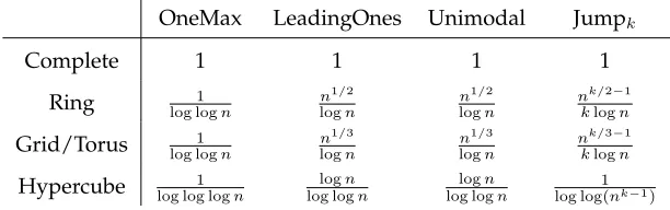
[image:19.612.162.468.110.206.2]Hypercube log log log1 n log loglognn log loglognn log log(1nk−1)
Table 2: Comparison of upper bounds on the communication efforts: the table shows the asymptotic ratio of upper bounds on the communication effort from the rightmost column of Table 1 for the best fixed choice ofτ and the best adaptive Scheme based on bounds from Table 1. A value less than 1 indicates that the best fixedτ leads to better bounds, and a value larger than 1 indicates a decrease of the upper bound on the communication effort by the stated factor. In all casesλwas chosen as the largest pos-sible value that guarentees a linear speedup according to the above-mentioned upper bounds.
Given a fixed number of islands λ, we define the best τ as the largest τ that does not asymptotically increase the bound for the parallel time (compared toτ = 1). This assures good scalability while minimising the communication effort. For the ex-ample proposed the best τ is τ = Θ(logλn). This leads to E [Tpar] = O(nlogn
λ )and
E [Tcom] =O(|E| τ ·E [T
par]) =O(λ2 τ ·E [T
par]) =O(λ2n). The results for other topolo-gies and problems are summarised in Table 1. Notice that fixingτ to its best value is possible, provided that the number of island is small enough. Particularly for the ex-ample proposed the number of islands must beλ=O(logn)in order for the bestτ to be defined (τ ≥1).
For OneMax and LO, lower bounds on the expected parallel times in Table 1 follow from general lower bounds on the class of mutation-based evolutionary algo-rithms [27]: every mutation-based algorithm needs at leastΩ(nlogn)function evalua-tions on OneMax and at leastΩ(n2)function evaluations on LO. The parallel (1+1) EA withλislands makesλevaluations in one generation, hence the above bounds translate toE [Tpar] = Ωnlogn
λ
for OneMax andE [Tpar] = Ωn2
λ
for LO. Lower bounds for the communication efforts for fixed migration intervals come from the lower bound in Theorem 1; the floor function can be ignored in the asymptotic notation as in all cases of Table 1,E [Tpar]/τ = Ω(1), implyingE [⌊Tpar/τ⌋]≥E [Tpar/τ−1] = Ω(E [Tpar/τ]).
6.3 Adaptive scheme
In order to calculate the parallel time for the adaptive Scheme A we can refer to the results for the fixed scheme whenτ = 1, as shown in Theorem 3. For example, our Scheme A running on a complete topology solves OneMax in time O(nlogλ n +n). Scheme B has asymptotically the same parallel time of Scheme A, as shown in The-orem 8.
thus makes the same expected number of function evaluations, compared to a single island. In the example proposed linear speedup is achieved for a number of islands up toλ=O(logn), in fact for a larger number of islands the upper bound on the parallel time would beO(n)regardless ofλ. The bounds onλlimit the best upper bound on the parallel time achievable with our analytical framework. Table 1 shows the bound onλ
for different problems and topologies and the best achievable parallel time bound. For OneMax and LO, lower bounds on the expected parallel times in Table 1 follow from general lower bounds on the class of mutation-based evolutionary algorithms [27]
In order to calculate the communication effort we use Theorem 6 and 8 for Schemes A and B, respectively. We first get a general bound for everyλincluded in the linear speedup bound, and then we calculate it for the maximum value ofλ, thus providing the communication effort for the value ofλleading to the best achievable parallel time. Table 1 shows all results derived in this manner. In the following we provide an example of this calculation for Scheme A on LO.
6.3.1 Example: Communication effort of Scheme A for LO
We provide details on how to calculate bounds on the expected communication effort for Scheme A using Theorem 6, choosing LO as an example. Calculations for other test functions are similar. The purpose is to illustrate how we derived the results in Table 1.
In the following, λis restricted to the cases leading to linear speedup as stated below and in Table 1. The calculations often use thatlog(a+b+c)≤log(3 max(a, b, c)).
• For the complete topology (λ=O(n))
E(TAcom)≤λ(λ−1) n−1 X
j=0
log2 +en
λ
≤λ(λ−1)
n−1 X
j=0 log
2en
λ
=Oλ2nlogn
λ
.
If we setλ= Θ(n),
E(TAcom) =O(n3).
• For ring (λ=O(n1/2))
E(TAcom) =λ n−1 X
i=0
log 3
s1i/2
+ 1
λsi
+λ
!
≤λ
n−1 X
i=0
log3(en)1/2+en
λ +λ
≤λ
n−1 X
i=0 log
9en
λ
=Oλnlogn
λ
.
If we setλ= Θ(n1/2)we obtain
• For the grid (λ=O(n2/3)) we get
E(TAcom) = 4λ n−1 X
i=1
log 3
s1i/3 +
1
λsi
+ 2√λ
!
=Oλnlogn
λ
.
If we setλ= Θ(n2/3)
E(TAcom) =O(n5/3logn).
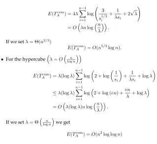
• For the hypercubeλ=O n
logn
E(TAcom) =λ(logλ) n−1 X
i=1 log
2 + log
1
si
+ 1
λsi
+ logλ
≤λ(logλ)
n−1 X
i=1
log2 + log (en) +en
λ + logλ
=Oλ(logλ)nlogn
λ
.
If we setλ= Θ n
logn
we get
E(TAcom) =O(n2log logn)
6.4 Evaluation of Results
[image:21.612.134.453.130.423.2]Recall that Table 1 only shows results for linear speedups, hence all (upper bounds on) parallel times are equal, but the range ofλvalues varies between topologies.
Table 2 compares upper bounds from Table 1 on the communication efforts for the best fixed value ofτagainst our adaptive schemes. For OneMax on all topologies the upper bound on the communication effort is by a small O(log logn)term larger for the adaptive schemes, compared to the best fixedτ. The latter varies according to the topology: it isτ = ((logn)/λ)2 for the ring,τ = ((logn)/λ)3/2 for the grid, and
τ= (logn)/λfor the hypercube and the complete graph. So, the additionalO(log logn) factor is a small price to pay for the convenience of adaptingτautomatically.
For LO, Scheme A on the ring has a communication effort ofO(n3/2logn) com-pared toΘ(n2), and for the grid it isO(n5/3logn)versusΘ(n2). Since the bounds for fixedτ are tight we see an improvement ofΩ(n1/2/logn)and Ω(n1/3/logn) respec-tively. These significant improvements show that decreasing the migration interval is an effective strategy in lowering the communication costs, without harming the par-allel running time. For the hypercube the communication effort is lower by a factor ofΩ(log(n)/log logn), whereas for the complete graph no differences are visible in the upper bounds.
for the communication effort. For the hypercube the upper bound on the communica-tion effort is lower by a factor ofO(log(n)/log logn), whereas for the complete graph no differences are visible in the upper bounds.
For Jump, with regard to comparing upper bounds, there are no differences for the complete graph, while on the hypercube Scheme A is by aO(log log(nk−1))factor worse than the best fixed value. For rings and grids the adaptive scheme is better; the performance gap even grows withkand hence the difficulty of the function.
Comparing Schemes A and B in Table 1, both achieve similar results. For LO we see an advantage of Scheme B over Scheme A: the general bound for the communica-tion effort of Scheme A isO(λ2nlog(n/λ)), whereas that for Scheme B isO(λ2n). This makes sense as the probability for finding an improvement in one generation is of or-derΘ(λ/n)for the consideredλ, and the ideal value for the migration interval is in the region ofΘ(n/λ). Scheme A needs to increase the migration interval aroundlog(n/λ) times to get into this range, which is precisely the performance difference visible in our upper bounds. The difference disappears forλ= Θ(n).
The same argument also applies to the more general function class of unimodal functions.
7
Discussion
The adaptive schemes presented here were designed to reduce the communication ef-fort without compromising exploitation. The results from Section 6.3 have demon-strated that this goal is achieved for functions that require a high degree of exploitation and little or no exploration. In settings where more exploration and less exploitation is needed, our schemes may not be able to find optimal or near-optimal migration inter-vals.
As mentioned in Section 1.1, the function class LOLZ from [13] was the first con-structed example where island models excel over panmictic populations and indepen-dent runs. Its structure is similar to the LO problem in a sense that bits have to be fixed to their correct values from left to right. In addition, LOLZ contains a number of traps that islands may fall into. For any island that has not got stuck in a trap, the probability of finding a fitness improvement is always at least1/(en)as for LO.
Solving LOLZ efficiently requires a delicate choice of the migration interval: for
τ = n5/3 the parallel (1+1) EA finds global optima on LOLZ efficiently with over-whelming probability, given appropriate parameter settings for the islands model (number of islands and communication topology) [13, Theorem 3]. This value of τ
is large enough to allow islands to explore different regions of the search space inde-pendently. But it is also small enough in order to propagate solutions of islands that are on target to finding the optimum, which then take over islands that have got stuck in local optima.
τ = O(n/λ)as deviations to larger values are very unlikely (cf. the first statement of Lemma 7). The same also holds for Scheme A.
However, as the diameter of the complete topologyKλis 1, we are then in a realm
whereτ = O(n/(λ·diam(Kλ))), and the island model is known to be inefficient [13,
Theorem 1]. The reason is that migration happens too frequently, and the island model behaves similarly to a panmictic population, which is prone to get stuck in a trap. Here our schemes, for complete topologies, would focus too much on exploitation, and not give the necessary degree of exploration needed to optimise LOLZ.
L¨assig and Sudholt [14, Section 6.1] also studied an instance of the Eulerian Cycle problem, where a large migration interval is beneficial as it leads to a better exploration. The same arguments as above lead to the same conclusion: our schemes typically will not give the necessary degree of exploration, leading to sub-optimal performance for complete topologies.
For sparse topologies like rings, however, exploration is increased and the situ-ation may improve. It is still unlikely that the recommended choice ofτ = n5/3 for LOLZ is being reached, as migration intervals are likely to remain in theO(n)range for most of the time (by similar arguments as for the first statement of Lemma 7). But we conjecture that for sufficiently largeλand sparse topologies a sufficient degree of exploration can be achieved. A detailed, formal analysis is beyond the scope of this paper and is left as an open problem for future work.
8
Conclusions and Future Work
We have presented two adaptive schemes for adapting the migration interval in island models. Both schemes have been accompanied by analytical frameworks that yield up-per bounds on the expected parallel time and the expected communication effort, based on probabilities of fitness improvements in single islands running elitist EAs. The re-sults show that our schemes are able to decrease the upper bound on the communica-tion effort without significantly compromising exploitacommunica-tion. For arbitrary topologies, we got upper bounds on the expected parallel time which are asymptotically no larger than those for maximum exploitation, that is, migration in every generation.
Example applications to the parallel (1+1) EA on common example functions re-vealed that, in the realm of linear speedups and comparing against the best fixed choice of the migration interval, the upper bound on the expected communication effort was larger by a tinyO(log logn)term for OneMax and similarly for the hypercube on Jump, but significantly lower for a general analysis of unimodal functions, and for rings and grids on Jump. For LO the adaptive Scheme A on grid and ring topologies can even guarantee an upper bound on the communication effort which is polynomially lower than the lower bound for the best fixed choice of the migration interval.
for a given problem. And it might be possible to further refine our schemes to allow an explicit tuning of the balance between exploitation and exploration.
Finally, this work presents mostlyupper boundsfor the expected running time and just upper bound for the expected communication effort of the adaptive schemes. Ob-taining correspondinglower boundswould help to identify what performance can be achieved, and assist in the search for provably optimal communication strategies. A promising direction is using black-box complexity [8, 17], which describes universal lower bounds on the expected (worst-case) running time ofeveryblack-box algorithm on a given class of functions. Recent advances towards a black-box complexity for par-allel and distributed black-box algorithms have been made [5, 6], which include island models using mutation for variation.
Acknowledgments:
The authors would like to thank Joseph Kempka and the participants of Dagstuhl seminar 13271 “Theory of Evolutionary Algorithms” for fruitful discussions and the anonymous reviewers for their constructive comments. Andrea Mambrini was par-tially funded by EPSRC (Grant No. EP/I010297/1). The research leading to these re-sults has received funding from the European Union Seventh Framework Programme (FP7/2007-2013) under grant agreement no 618091 (SAGE).
References
[1] E. Alba. Parallel evolutionary algorithms can achieve super-linear performance.
Information Processing Letters, 82(1):7–13, 2002.
[2] E. Alba and G. Luque. Theoretical models of selection pressure for deas: topology influence. In IEEE Congress on Evolutionary Computation (CEC 2005), volume 1, pages 214–221 Vol.1, 2005.
[3] E. Alba, G. Luque, and S. Nesmachnow. Parallel metaheuristics: Recent advances and new trends.International Transactions in Operational Research, 20(1):1–48, 2013.
[4] L. Araujo and J. J. Merelo Guerv ´os. Diversity through multiculturality: Assess-ing migrant choice policies in an island model. IEEE Transactions on Evolutionary Computation, 15(4):456–469, 2011.
[5] G. Badkobeh, P. K. Lehre, and D. Sudholt. Unbiased black-box complexity of par-allel search. In13th International Conference on Parallel Problem Solving from Nature (PPSN 2014), volume 8672 ofLNCS, pages 892–901. Springer, 2014.
[6] G. Badkobeh, P. K. Lehre, and D. Sudholt. Black-box complexity of parallel search with distributed populations. In Proceedings of Foundations of Genetic Algorithms (FOGA 2015). ACM Press, 2015. To appear.
[7] Y. Bravo, G. Luque, and E. Alba. Influence of the migration period in parallel distributed GAs for dynamic optimization. InLearning and Intelligent Optimization (LION ’12), pages 343–348. Springer, 2012.
[9] T.-P. Hong, W.-Y. Lin, S.-M. Liu, and J.-H. Lin. Experimental analysis of dynamic migration intervals on 0/1 knapsack problems. InIEEE Congress on Evolutionary Computation (CEC 2007), pages 1163–1167, 2007.
[10] J. L¨assig and D. Sudholt. General scheme for analyzing running times of parallel evolutionary algorithms. In11th International Conference on Parallel Problem Solving from Nature (PPSN 2010), volume 6238 ofLNCS, pages 234–243. Springer, 2010.
[11] J. L¨assig and D. Sudholt. Adaptive population models for offspring populations and parallel evolutionary algorithms. InProceedings of the 11th Workshop on Foun-dations of Genetic Algorithms (FOGA 2011), pages 181–192. ACM Press, 2011.
[12] J. L¨assig and D. Sudholt. Analysis of speedups in parallel evolutionary algorithms for combinatorial optimization. In22nd International Symposium on Algorithms and Computation (ISAAC 2011), volume 7074 ofLNCS, pages 405–414. Springer, 2011.
[13] J. L¨assig and D. Sudholt. Design and analysis of migration in parallel evolutionary algorithms. Soft Computing, 17(7):1121–1144, 2013.
[14] J. L¨assig and D. Sudholt. Analysis of speedups in parallel evolutionary algorithms and (1+λ) EAs for combinatorial optimization.Theoretical Computer Science, 551:66– 83, 2014.
[15] J. L¨assig and D. Sudholt. General upper bounds on the running time of parallel evolutionary algorithms. Evolutionary Computation, 22(3):405–437, 2014.
[16] P. K. Lehre. Fitness-levels for non-elitist populations. In Proceedings of the 13th Annual Genetic and Evolutionary Computation Conference (GECCO ’11), pages 2075– 2082. ACM Press, 2011.
[17] P. K. Lehre and C. Witt. Black-box search by unbiased variation. Algorithmica, 64(4):623–642, 2012.
[18] W.-Y. Lin, T.-P. Hong, S.-M. Liu, and J.-H. Lin. Revisiting the design of adaptive migration schemes for multipopulation genetic algorithms. In2012 Conference on Technologies and Applications of Artificial Intelligence (TAAI), pages 338–343, 2012.
[19] G. Luque and E. Alba. Parallel Genetic Algorithms–Theory and Real World Applica-tions, volume 367 ofStudies in Computational Intelligence. Springer, 2011.
[20] A. Mambrini and D. Sudholt. Design and analysis of adaptive migration intervals in parallel evolutionary algorithms. InProceedings of the Genetic and Evolutionary Computation Conference (GECCO 2014), pages 1047–1054. ACM Press, 2014.
[21] A. Mambrini, D. Sudholt, and X. Yao. Homogeneous and heterogeneous island models for the set cover problem. In Parallel Problem Solving from Nature (PPSN 2012), volume 7491 ofLNCS, pages 11–20. Springer, 2012.
[23] K. Osorio, E. Alba, and G. Luque. Using theory to self-tune migration periods in distributed genetic algorithms. InIEEE Congress on Evolutionary Computation, pages 2595–2601, 2013.
[24] K. Osorio, G. Luque, and E. Alba. Distributed evolutionary algorithms with adap-tive migration period. In11th International Conference on Intelligent Systems Design and Applications (ISDA ’11), pages 259–264, 2011.
[25] G. Rudolph. Takeover time in parallel populations with migration. In Proceed-ings of the 2nd International Conference on Bioinspired Optimization Methods and Their Applications (BIOMA 2006), pages 63–72, 2006.
[26] Z. Skolicki and K. De Jong. The influence of migration sizes and intervals on island models. InProceedings of the Genetic and Evolutionary Computation Conference (GECCO 2005), pages 1295–1302. ACM, 2005.
[27] D. Sudholt. A new method for lower bounds on the running time of evolutionary algorithms. IEEE Transactions on Evolutionary Computation, 17(3):418–435, 2013.
[28] M. Tomassini. Spatially Structured Evolutionary Algorithms: Artificial Evolution in Space and Time. Springer, 2005.