A durability performance-index for concrete: developments in a novel test method

This is a repository copy of A durability performance-index for concrete: developments in a novel test method.

White Rose Research Online URL for this paper: http://eprints.whiterose.ac.uk/97597/

Version: Accepted Version Article:

McCarter, WJ, Chrisp, TM, Starrs, G et al. (4 more authors) (2015) A durability performance-index for concrete: developments in a novel test method. International Journal of Structural Engineering, 6 (1). pp. 2-22. ISSN 1758-7328

https://doi.org/10.1504/IJSTRUCTE.2015.067966

[email protected] https://eprints.whiterose.ac.uk/

Reuse

Unless indicated otherwise, fulltext items are protected by copyright with all rights reserved. The copyright exception in section 29 of the Copyright, Designs and Patents Act 1988 allows the making of a single copy solely for the purpose of non-commercial research or private study within the limits of fair dealing. The publisher or other rights-holder may allow further reproduction and re-use of this version - refer to the White Rose Research Online record for this item. Where records identify the publisher as the copyright holder, users can verify any specific terms of use on the publisher’s website.

Takedown

If you consider content in White Rose Research Online to be in breach of UK law, please notify us by

Reference to this paper should be made as follows: McCarter, W.J., Chrisp, T.M.,

Starrs, G., Basheer, P.A.M., Nanukuttan, S., Srinivasan, S. and Magee, B.J. (2015)

A DURABILITY PERFORMANCE-INDEX FOR CONCRETE:

DEVELOPMENTS IN A NOVEL TEST METHOD

ABSTRACT

Implementation of both design for durability and performance-based standards and

specifications are limited by the lack of rapid, simple, science-based test methods for

characterizing the transport properties and deterioration resistance of concrete. This paper

presents developments in the application of electrical property measurements as a testing

methodology to evaluate the relative performance of a range of concrete mixes. The technique

lends itself to in-situ monitoring thereby allowing measurements to be obtained on the

as-placed concrete. Conductivity measurements are presented for concretes with and without

supplementary cementitious materials (SCM's) from demoulding up to 350-days. It is shown

that electrical conductivity measurements display a continual decrease over the entire test

period and attributed to pore structure refinement due to hydration and pozzolanic reaction.

The term Formation Factor is introduced to rank concrete performance in terms of is

resistance to chloride penetration.

Keywords: concrete, cover-zone, durability, performance testing, monitoring, electrical

1.0 INTRODUCTION

European Standard EN206-1 (British Standards Institution, 2000a) deals with durability of

concrete entirely on the basis of prescriptive specification of minimum grade, minimum

binder content and maximum water-binder ratio for a series of well-defined environmental

classes. Annex J within this code does give brief details of the approach and principles for

performance-related design methods with respect to durability. Although numerous attempts

have been made to introduce performance-based specifications, this has been hampered by

the lack of reliable, consistent and standardised test procedures and protocols for evaluating

concrete performance (Bentur and Mitchell, 2008). The Committee responsible for

developing EN-206 recognised that an appropriate testing technology has not been

sufficiently developed to satisfy performance-based philosophy (Hobbs, 1998). In this

respect, there is widespread recognition that central to the concept of performance-based

specifications is the requirement for reliable and repeatable test methods which can evaluate

the required performance characteristic(s) along with performance compliance limits, which

should take into account the inherent variability of the test method. It is evident that test

procedures are required such that those properties of concrete which ensure long-term

durability can be determined very early on in the life of a structure and that it will meet

specified requirements (DuraCrete, 1999). The lack of adequate performance-related test

methods is one of the main factors inhibiting the move from the prescriptive, deem-to-satisfy,

approach to performance-based specifications.

Further to the above, there is also an intense need to evaluate the concrete earlier to obtain an

early indication of potential concerns or, conversely, to gain early confidence that all is well.

The sooner information is obtained about the early-age properties of any given batch of

concrete, the sooner adjustments can be made to the materials, proportions or processes for

subsequent concrete placement and the sooner remedial measures can be initiated on the

concrete already installed or construction practices altered (e.g. extended curing). Early-age

testing is useful in this regard and, indeed, absolutely essential as the consequences of

unsatisfactory concrete discovered at a later stage becomes expensive. The term identity

testing is used in BS 8500-1 (British Standards Institution, 2006a) to describe testing to

validate the identity of the mix. Identity testing attempts to verify some key characteristic of

the concrete that relates to the desired performance and could take the form of a slump, flow,

density, strength, water-content or some non-destructive or in-place method. For example,

diffusivity of, say, 310-12 _m2_{/s, assuming that the mix had been pre-qualified based on}

preconstruction testing. During actual construction the challenge is to perform a test - or suite

of tests - on concrete sampled at the time of placement which can then be used to verify that

the concrete, as delivered, is substantially the same as the concrete that had previously been

shown to meet the 310-12 m2/s diffusivity requirement. There would, in addition, be a need to assess that the in-place concrete has a diffusivity of 310-12 m2/s using appropriate testing techniques.

Sustainable concrete construction requires performance-based knowledge of expected

durability and service-life; as a result, the quantification of concrete performance by means a

single, easily measurable parameter is a subject of increasing interest. Moreover, since it is

the cover-zone concrete which protects the steel from the external environment, the

protective properties of this zone is crucial in attempting to make predictions as to the

performance of the structure with regard to likely deterioration rates for a particular exposure

condition and compliance with specified service-life. Regarding cover-zone properties, it is

the permeation properties which are important and terms such as diffusivity, permeability and

sorptivity are used in this respect. There clearly exists a need to study and determine

quantitatively those near-surface characteristics of concrete which promote the ingress of

gases or liquids containing dissolved contaminants and defining concrete performance in

terms of a durability parameter which gives an assessment of these properties. Furthermore,

evaluation of the long-term performance of the concrete without information on the in-situ

properties of the prepared/placed concrete could result in an erroneous response.

To this end, developments in the use of electrical property measurements are presented as

offering a potential performance-based testing technique and methodology for indexing the

protective qualities of cover-zone concrete.

2.0 BACKGROUND AND RATIONALE

2.1 Electrical properties of porous materials

Conductivity is a fundamental property of a material and is related to the resistance, in ohms,

between opposite faces of a unit cube of that material. If R is the bulk resistance of a

prismatic sample of concrete contained between a pair of electrodes of area A (cm2), separated by a distance L (cm), then its bulk conductivity, , is given by,

     

 L

Since the flow of water under a pressure differential (hence permeability) or the movement of

ions under a concentration gradient (hence diffusion) is analogous to the flow of current

under a potential difference (hence electrical resistance), it is understandable that the

electrical properties of concrete could serve as a simple, yet effective, testing technique for

assessing transport processes, hence performance and durability. Drawing an analogy

between hardened concrete and rock (as both could be regarded as porous solids),

conventional treatment of rock conductivity data has been to use the term formation factor (F)

which is defined as the ratio of the conductivity of the saturating liquid (p) to the bulk

conductivity of the saturated rock () and linked to porosity, , through the empirical

relationship (Archie, 1942),

m p

F 

 

(2)

In this relationship, the exponent m is related to the tortuosity and connectivity of the pore

network within the rock with m values lying, typically, in the range 1.5-2.5. Millington and

Quirk (Millington and Quirk, 1962) have presented a relationship relating rock permeability,

k (m2), to F and the average pore radius, r, within the rock determined by mercury intrusion porosimetry as: k 8 r F 2  (3)

The Katz-Thomson model (Katz and Thomson, 1986) for saturated porous systems

introduces the term critical pore diameter and establishes a relationship between the

permeability, k (m/s), formation factor, F, and the critical pore diameter, dc, within the system

as,         g d k 226 1

F 2c (4)

where is the density of water; g is the gravitational acceleration and  the viscosity of the

permeating fluid.

If the solid phase can be regarded as non-conductive in comparison to that of the interstitial

pore-fluid, diffusivity and ionic conductivity of a saturated porous system are connected

through the Nernst-Einstein relationship (see, for example, Atkinson and Nickerson, 1984;

Christensen et al, 1994; Kyi and Batchelor 1994; Tumidajski and Schumacher 1996; Lu,

(5)

where D is the diffusion coefficient of the porous system; Do the diffusion coefficient of the

ion (e.g. Cl-) in the free electrolyte, and  is termed the tortuosity; the ratio p thus

represents the reciprocal of the formation factor.

2.2 Further Considerations

From an electrical point of view, concrete can be regarded as a composite comprising

non-conductive aggregate particles embedded in an ionically conducting cementitious matrix. As

a consequence, the hydration process will result in time-variant microstructural changes

which will decrease capillary pore diameter, decrease in pore connectivity and increase pore

tortuosity. Long-term pore structure refinement, beyond the post-curing period, will thus

influence permeation properties and must be evaluated. This is particularly important for

concretes containing supplementary cementitious materials (SCM) such as fly-ash or ground

granulated blast-furnace slag.

In order to fully exploit electrical property measurements in assessing the relative

performance of different concrete mixtures, the conductivity of the pore-fluid, p, is required.

For example, two concretes, with exactly the same underlying microstructure, could display

different bulk conductivities due to differing pore-fluid chemistry which could, for example,

result from differing ionic concentrations within the saturating pore fluid. This is particularly

relevant when SCM's are used as these materials alter the concentrations of Na+_{, K}+ _{and OH}

-within the interstitial aqueous phase in comparison to a plain Portland cement concrete.

In order to estimate the conductivity of the pore-fluid, pore expression techniques can be used

(Barneybeck and Diamond, 1982). This is impractical for a variety of reasons, not least

because it complicates the testing procedure. Furthermore, pore expression techniques are

more applicable to cement-paste samples (not concretes) with relatively high water/binder

ratios at the early stages of hydration. Under such circumstances, the pore-fluid conductivity

could be estimated from the ionic concentration predicted from a model. For example, the

model of Taylor (Taylor, 1987) predicts the concentration of various ionic species in the pore

solution based on the cement composition and degree of hydration, and has been shown to be

reasonably accurate (Reardon, 1992). From the estimated concentrations it is then possible to

(Snyder et al, 2003) and Bentz (Bentz, 2007) is used to estimate the conductivity of the pore

fluid and discussed below.

3.0 EXPERIMENTAL

3.1 Embedded Electrode Array

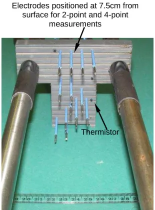
To facilitate electrical measurements within the cover-zone, the Authors have modified a

multi-electrode array (McCarter et al, 1995; Chrisp et al, 2002) which is embedded within

concrete specimens at the time of casting. The array allows monitoring of the spatial

distribution of both electrical resistance and temperature within the cover region. In

summary, the array comprises six electrode-pairs mounted on a 'T-shaped' PVC former, with

the former being secured on two steel bars (1.5cm diameter) as shown in Figure 1; the

cover-to-steel is 5.0cm. Four thermistors were also mounted on the array for temperature

measurement.

The pairs of electrodes were positioned at discrete distances from the base of the former and

were located at 1.0, 2.0, 3.0, 4.0, 5.0 and 7.5cm from the concrete surface. A further two

electrodes were positioned at a depth of 7.5cm which, together with the electrode-pair

positioned at 7.5cm, formed a set of four co-linear electrodes with a 1.0cm spacing (see

Figure 1. This configuration allowed 4-point electrical measurements at this depth and the

conductivity of the concrete,  (S/cm) could then be evaluated from the relationship

(McCarter et al, 2009),

where s is the spacing between the electrodes (=1cm) and R4pt is the measured 4-point

resistance, in ohms (). Electrical measurements obtained at 7.5cm are sufficiently remote

from any effects at the concrete surface (e.g. drying, wetting) and will reflect cement

hydration, pozzolanic reaction and microstructural development. This is discussed below.

The conductivity of the concrete at each electrode-pair can be evaluated by multiplying the

measured resistance by a calibration factor (denoted kf). This was obtained by calibrating

with the measured conductivity of 10cm cubes cast from the same batch as the slabs used in

the experimental programme (three cubes per mix). These cubes had four, embedded stainless

steel pins to the same specification as those on the arrays. The pins were positioned centrally

within the cube in a co-linear fashion and a centre-to-centre spacing of 1.0cm (i.e. the same

obtained per cube. A 4-point technique using external stainless steel plates and the internal

electrodes was used for evaluation of the concrete conductivity (McCarter et al, 2009) and

subsequent evaluation of the electrode-pair calibration factor. Hence the measured resistance,

R (ohms), across the electrode-pairs on the array could be converted to conductivity,  (in

S/cm), through the relationship,

S/cm (7)

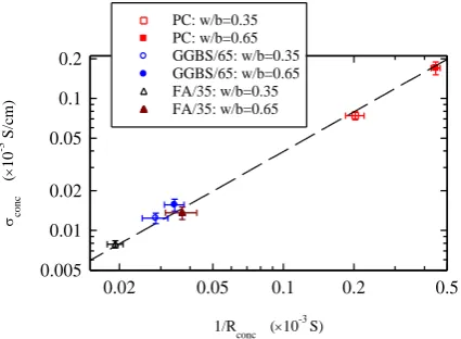
Figure 2 presents the calibration curve for the electrode-pair geometry used within the

experimental programme with x and y error-bars representing one standard deviation; in those

cases where the error bar appears to be missing, the data markers are larger than the error bar.

In this Figure, the conductance (=1/Rconc, in Siemens) measured across the electrode-pairs

within the concrete cubes is plotted against the conductivity of the concrete, conc, with the

slope of the straight line being the calibration factor and is equivalent to the ratio L/A in

equation (1) above. kf was evaluated as 0.412cm-1. The conductivity value was further

cross-checked with 4-point measurements obtained from electrodes positioned at 7.5cm on the

array.

3.2 Materials and Sample Preparation

The concrete mixes used within the experimental programme are presented in Table 1. The

binders comprised Portland cement (PC) clinker, CEM I to EN197-1:2000 (British Standards

Institution, 2000); CEM I cement blended with ground granulated blast-furnace slag (GGBS)

to EN15167-1 (British Standards Institution, 2006); and CEM I cement blended with

low-lime fly-ash (FA) to EN450-1 (British Standards Institution, 2005). Crushed granite

aggregate was used throughout. A mid-range water reducer/plasticiser (SikaPlast 15RM)

conforming to EN934-2 (British Standards Institution, 2009) was added by percentage mass

of binder. The PC and SCM's were combined at the concrete mixer. The oxide analysis of the

SCM's is presented in Table 2.

Specimens were cast as 25×25×15cm (thick) slabs in steel formwork; the 25×25cm face cast

against the formwork – which was to be used as the working face – had a small dyke cast

around it to facilitate ponding. An electrode array was positioned at the plan centre of each

slab with the steel reinforcing projecting out through the sides of the specimens; wiring from

the embedded array was ducted out of the slab and terminated with a multipole D-connector.

- six for compressive strength tests and three for calibration tests noted above. The 28-day

and 180-days compressive strength is presented in Table 1 (f28 and f180, respectively, in MPa).

3.3 Testing Regime and Monitoring

On demoulding at approximately 24-hours, each slab specimen was wrapped in damp hessian

and placed in a heavy-duty polythene bag which was then sealed. The specimens were left in

a laboratory at constant temperature (20±1ºC) for a period of 27-days. At this time, the four

vertical faces (25×15cm) of the specimens were painted with two coats of a proprietary

sealant and exposed to a laboratory environment 20±1ºC, 55%±5%RH. After approximately

7-days, all samples were ponded with water for a period of 24-hours. This ensured the surface

region of all specimens was in a similar saturated state. Samples were then allowed to dry for

a further 7-days before being subjected to a cyclic ponding regime with salt solution to

simulate natural environmental action. This regime was, generally, 1-day ponding followed

by 6-days drying in the laboratory environment. A 0.55 Molar salt solution was used

throughout (32g of sodium chloride per litre of distilled water).

Electrical resistance measurements were obtained by connecting the samples to a

multiplexing system and an auto-ranging data logger. The resistance of the concrete between

each electrode-pair was obtained a fixed frequency of 1kHz; the signal amplitude was 350mV

with a measurement integration time of 1.0 second. Thermistor measurements were also

acquired using the same system which were subsequently converted to temperature in degrees

Celsius. On demoulding at 24-hours, measurements were taken continuously on a 12-hour

cycle for the duration of the test period. Periodically, 4-point measurements at 7.5cm were

obtained manually using an Agilent 4263B LCR meter.

4.0 RESULTS AND DISCUSSION

4.1 Preliminaries

This paper focusses on the response from the electrode-pairs positioned at 7.5cm from the

exposed surface of the specimens as, at this depth, they are sufficiently distant from the

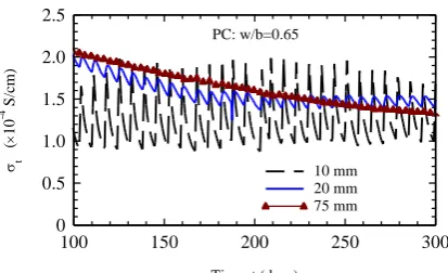
surface to be unaffected by the wetting/drying action at the surface. To highlight this point,

Figure 3 presents the conductivity, t, versus time response for the electrodes positioned at

1.0, 2.0 and 7.5cm from the surface for the PC concrete mix (w/b=0.65). For illustrative

purposes, data are presented between 100 and 300 days after casting. For reasons of clarity,

wetting/drying regime on the conductivity of the concrete is clearly evident for the electrodes

positioned 1.0cm and 2.0cm from the surface, with periods of wetting resulting in an increase

in conductivity and drying accompanied by a decrease in conductivity. The electrodes

positioned at 7.5cm, however, display a continual decrease with time and remain unaffected

by wetting/drying at the concrete surface. Similar responses were obtained for the other

concrete mixes and it is for this reason that measurements from the electrode-pair positioned

at 7.5cm from the exposed surface, and still within the near-surface region, are presented

within this paper.

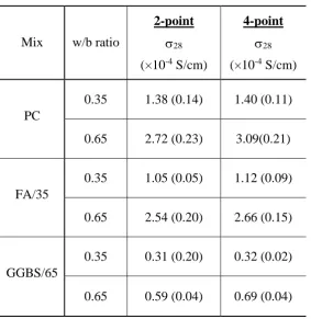
Based on the resistance values obtained at each electrode-pair positioned within the surface

7.5cm, and using equation (7) above, the average 28-day conductivity for the concrete within

the surface 7.5cm is presented Table 3. Also presented in Table 3 are the conductivity values

evaluated at 7.5cm using 4-point resistance measurements and equation (6) above. Both

methods show good agreement in estimating the concrete conductivity at this position within

the cover-zone.

4.2 Temporal change in conductivity

Electrical conduction through concrete will be primarily via the connected capillary porosity

within the binder which, itself, will be influenced by hydration and pozzolanic reaction. This

will result in time-variant microstructural changes to the pore network and will be reflected in

a temporal decrease in the measured conductivity. The conductivity (t) of the concrete mixes

in Table 1 is presented in Figures 4 and 5 and, as noted above, based on the values obtained

from the electrode-pair positioned at 7.5cm.

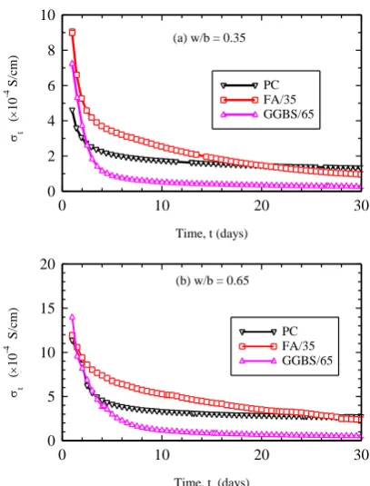
Figure 4(a) displays the variation in conductivity for concrete mixes with w/b=0.35 over the

initial 27-days after demoulding. In general terms, the conductivity of all mixes display a

continual decrease although the influence of binder composition on conductivity is also

clearly evident during the initial curing period. For periods <3 days, the PC concrete displays

a lower conductivity than the FA/35 and GGBS/65 concrete mixes and reflects the initial

slower reaction of these blended systems. However, for periods >3-days, the conductivity of

the GGBS/65 concrete achieves lower values than the PC concrete whereas for the FA/35

concrete, this effect does not occur until approximately 15 days. Similar trends are observed

in Figure 4(b) for concrete mixes with w/b=0.65 although the conductivity of the FA/35 mix

observed that an increase in the w/b ratio results in an increase in the conductivity of the

concrete.

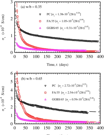
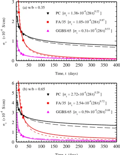
Figures 5(a) and (b) display the conductivity (at 7.5cm from the surface) from 10-days up to

approximately 350 days for, respectively, 0.35 and 0.65 w/b ratio. It is during this period that

curing measures were removed (at 28-days) from the specimens and the surface subjected to

a cyclic wetting and drying regime. It is apparent that this has not had any effect on the

conductivity of the concrete at this depth as there are no 'abrupt' changes in the conductivity

at 28-days and the ensuing period; this further corroborates the discussion of Figure 3 above.

Both Figure 5(a) and (b) display a continual decrease in conductivity over the entire period

indicating on-going hydration and pozzolanic reaction.

The influence of SCM's on the conductivity is clearly displayed in these Figures; at the end of

the test period, the conductivity of the FA/35 and GGBS/65 concrete mixes are almost an

order of magnitude less than the PC concrete mix, at both w/b ratios. The decrease in

conductivity for both the slag and fly-ash concretes reflects the on-going pore structure

refinement during the post-curing period. Although such concretes may not necessarily be of

lower total porosity than the PC concretes, it is of a much more discontinuous and tortuous

nature, due to the ongoing reactions within the existing pore structure (Li and Roy, 1986).

The decrease in conductivity for the concretes presented in Figure 5 can be represented by the

equation:

(8)

where, t is the conductivity at time, t (in days); ref is the conductivity at a reference time,

tref, and n is an exponent related to hydration and pozzolanic reaction. The reference time for

the current work is taken as 28-days, hence tref = 28 days and ref values are presented in

Table 3 (2-point). Best-fit curves to the data are plotted on Figure 5(a) and (b) as dashed lines

through the measurement points and the fitting equations are presented on these Figures. It is

interesting to observe that for a particular cementitious binder, the exponent, n, for both w/b

ratios are similar i.e. n is independent of w/b ratio.

Although the equations on these Figures were developed on the best-fit line to all the data

points for a particular w/b ratio (i.e. over 700 measurement points), a curve can be evaluated

from fewer measurements, which has obvious practical implications. For example, Figures

10, 20 and 28 days (3 measurement points) using the same reference time of 28-days. For

comparative purposes, the best-fit curves based on all the measurement points on Figure 5 are

also presented on Figure 6 (dashed lines).

4.3 Conductivity and Diffusion

Equation (5) above highlights the interrelationship between conductivity and diffusion

coefficient of a saturated porous material. A conductivity measurement must thus give an

indirect assessment of the instantaneous diffusion coefficient of the concrete. However, to

fully implement equation (5) the conductivity of the pore-water, p, must be known or, at

least, assessed.

Due to both the practicality and considerable difficulty in expressing pore solution from

concrete, the conductivity of the pore water can be estimated from the contributions to

conductivity of the major ions in the pore water, namely, sodium (Na+), potassium (K+) and hydroxyl (OH-). A straightforward procedure for estimating pore solution conductivity from the concentrations of these ions in the pore-water has been developed by Snyder (Snyder et

al, 2003) and Bentz (Bentz, 2007). In summary, for a particular degree of hydration, the

concentrations of Na+ and K+ in the pore-water are computed from the binder composition and assuming that 75% of the sodium and potassium initially present as oxides in the

cement-based materials will be released into the pore-water. The concentration of OH- is deduced from the electroneutrality condition. These data are then used to compute the pore solution

electrical conductivity, viz,

(9)

where zi, ci, and i are, respectively, the ionic species valence, molar concentration and

equivalent conductivity associated with each ion, i. The equivalent conductivity is then

computed from,

(10)

The values of - the equivalent conductivity of an ionic species at infinite dilution - and the

conductivity coefficient, Gi for Na+, K+, and OH- ions are presented in Table 4 (Snyder et al,

2003). The quantity IM is the ionic strength (molar basis) and has the following definition,

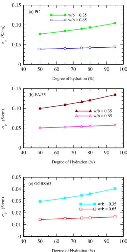
Based on this model, and the oxide analysis of the cementitious materials used in the

experimental programme (Table 2), the estimated conductivity values of the pore-water at

selected degrees of hydration are presented in Figures 7(a)-(c) for PC, FA/35 and GGBS/65

binders. Values are plotted over the range 50%-95% hydration which represents,

approximately, the degree of hydration over the time-scale 7-days to 180-days (Hewlett,

1998; Lin and Meyer, 2009). It is evident from Figure 7 that hydration has little effect on the

pore-water conductivity, particularly at the higher w/b ratio where the conductivity remains

virtually constant. At w/b=0.35, the conductivity of the pore-water increases by

approximately 30% as the degree of hydration increases from 50% to 95%.

From equations (5) and (8), it is now possible to obtain an approximation for the

instantaneous diffusion coefficient at time, t, denoted Di(t), as,

(12)

Consider the PC concrete with w/b=0.35. If, over the test period, an average degree of

hydration of 75% is assumed then, following the work of Snyder (Snyder et al, 2003), the

conductivity of the pore-water, p, is evaluated as 0.091S/cm. If the self-diffusion of the

chloride ion (Cl-) in pure water, Do, is assumed to be 1.84×10-9 m2/s (Li and Gregory, 1974;

Shackleford and Daniel, 1991), then, from Figure 5(a) and equation (12),

(13)

Hence,

(14)

Repeating the same process for the remaining mixes obtains the curves presented in Figures

8(a) and (b) and plotted on a log-log scale.

The diffusion coefficient obtained above would represent the instantaneous diffusion

coefficient and should not be confused with the effective diffusion coefficient, Deff, which is

generally referred to in the literature. Deff is normally obtained from the error function

solution to the chloride profile obtained from dust drillings taken through the cover-zone.

With reference to Figure 9, Deff represents the integrated, or time-averaged, diffusion

coefficient and would be related to the instantaneous diffusion coefficient, Di(t), by,

where tex is the concrete age at first exposure to chlorides. At short exposure times, Deff  Di ;

however, it is evident from Figure 9 that as the exposure time increases i.e. (t - tex) increases,

then Deff will tend to underestimate the diffusion coefficient at the time of measurement. If

Deff values are used to make predictions as to future chloride ingress they will tend to be

conservative estimates, i.e. they will underestimate the time to activation of corrosion.

It is accepted that the evaluation of the conductivity of the pore-water is, at best, approximate,

however, considering the extremely wide variation in published values for diffusion

coefficients for concretes with and without SCM's (Bamforth et al, 1997), evaluation of the

diffusion coefficient using this methodology could represent a good estimate.

4.4 Towards a Performance-Based Index

From the definition of formation factor (F) in equation (2) above, and the relationship of this

parameter with tortuosity and diffusivity through equation (5), it should be possible to rank

concrete in terms of its resistance to chloride penetration; in other words, the greater the F

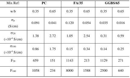
value, the better the performance of the concrete in terms of chloride resistance. Table 5

presents the computed F values for each concrete mix in Table 1 at both 28-days (F28) and

180-days (F180); as before, an average degree of hydration of 75% for each binder type has

been assumed throughout in calculating p.

With reference to Table 5, decreasing the w/b ratio from 0.65 to 0.35 results in,

approximately, a fivefold increase in F for each mix. Moreover, the beneficial effect of the

fly-ash and slag is clearly evident, particularly at longer time-scales. It is interesting to note

that whilst the GGBS/65 concrete displays the lowest bulk conductivity value, when the

conductivity of the pore-water is considered, it is out-ranked by the FA/35 concrete in the

longer-term.

5. CONCLUDING COMMENTS

The work detailed above has presented developments in the application of electrical property

measurements as a potential test method to rank the relative performance of a range of

concrete mixes. This was undertaken through a combination of bulk conductivity

measurements together with an estimated value for the pore-fluid conductivity; these values

were then used to assess concrete performance in terms of diffusivity and Formation Factor

(F). In general terms, the lower the F value for the concrete, the poorer its performance

The following general conclusions can be drawn:

(1) A 4-point and a 2-point technique were used to obtain the in-situ conductivity of the

concrete, with both methods giving similar values. Unlike the 4-point method, however, the

2-point method required prior calibration.

(2) A general equation has been presented to model the temporal decrease in conductivity. An

ageing factor was introduced to account for conductivity versus time response.

(3) The decrease in electrical conductivity reflected on-going hydration and pore structure

refinement within the binder and extended over the duration of the test programme (which

was approximately 350-days).

(4) Those concretes containing SCM's displayed a more marked decrease in conductivity than

the plain PC mix and was attributed to the pozzolanic reaction and resulting influence on the

REFERENCES

Archie G. E. (1942). 'The electrical resistivity log as an aid in determining some reservoir

characteristics', Trans. of the Amer. Inst. of Mining and Metallurgical Engrs., 146, 54-62.

Atkinson, A. and Nickerson, A. K. (1984). 'The diffusion of ions through water-saturated

cement', J. of Matls. Sci., 19(9), 3068-3078.

Bamforth, P. B., Price W. F. and Emerson, M. (1997). 'An international review of chloride

ingress into structural concrete', Transport Research Laboratory, Contractor Report 359,

162pp, (ISSN 0266-7045).

Barneyback, R.S. and Diamond, S. (1981). 'Expression and analysis of pore fluid from

hardened cement pastes and mortars', Cem. Concr. Res., 11(2), 279–285.

Bentur, A. and Mitchell D. (2008). 'Materials performance lessons', Cem. Concr. Res., 38(2),

259-272, (2008).

Bentz, D. (2007). 'A virtual rapid chloride permeability test', Cem. Concr. Comp., 29(10),

723-731.

British Cement Association, (1998). 'Minimum requirements for durable concrete', Ed. By D.

W. Hobbs, British Cement Association, 172pp.

British Standards Institution, EN206-1: (2000a). 'Concrete: Specification, performance,

production and conformity', BSI, London.

British Standards Institution, EN197-1. (2000b). 'Cement-Part 1: Composition, specifications

and conformity criteria for common cements', BSI, London.

British Standards Institution, EN450-1. (2005). 'Fly ash for concrete-Part 1: Definition, specifications and conformity criteria’, BSI, London.

British Standards Institution, BS8500-1. (2006a). 'Concrete-Complementary British Standard

to EN 206-1 – Part 1: Method of specifying and guidance for the specifer', BSI, London.

British Standards Institution, EN15167-1. (2006b). 'Ground granulated blast furnace slag for

use in concrete, mortar and grout — Part 1: Definitions, specifications and conformity

criteria', BSI, London.

British Standards Institution, EN934-2. (2009). 'Admixtures for concrete, mortar and grout.

Chrisp T. M., McCarter W. J., Starrs G., Basheer, P. A. M. and Blewett J. (2002). 'Depth

related variation in conductivity to study wetting and drying of cover-zone concrete', Cem.

Concr. Comp., 24(5), 415-427.

Christensen, B. J., Coverdale, R. T., Olsen, R. A., Ford, S. J., Garboczi, E. J., Jennings, H.

M., Mason, T. O. (1994). 'Impedance spectroscopy of hydrating cement-based materials:

measurement, interpretation, and applications', J. Amer. Ceramic Soc., 77(11), 2789-2804.

DuraCrete (1999). 'Compliance testing for probabilistic Design purposes' EU Brite-EuRam

III, Project Report BE95-1347/R8, 105pp (ISBN 903760420X).

Hewlett, P. C. (Editor) (1998). Chapter 4 in 'Lea's Chemistry of Cement',

Butterworth-Heinemann, Oxford, UK, 4th Edition (ISBN 0750662565).

Hobbs, D. W. (Editor) (1998). 'Minimum requirements for durable concrete: Minimum

requirements for durable concrete carbonation- and chloride-induced corrosion, freeze-thaw

attack and chemical attack, British Cement Association, 172pp (ISBN 0721015247,

9780721015248).

Katz, A. J. and Thompson, A. H. (1986). 'Quantitative prediction of permeability in porous

rock', Phys. Rev. B: Condensed Matter, 34(11), 8179-8181.

Kyi, A. A., Batchelor, B. (1994). 'An electrical conductivity method for measuring the effects

of additives on effective diffusivities in Portland cement pastes', Cem. Concr. Res., 24(4),

752-764.

Li, S. and Roy, D. M. (1986). 'Investigation of relations between porosity, pore structure, and Cl − diffusion of fly ash and blended cement pastes', Cem. Concr. Res., 16(5), 749-759.

Li, Y-H. and Gregory, S. (1974). 'Diffusion of ions in sea water and deep-sea sediments',

Geochimica et Cosmochemica Acta, 38, 703-714.

Lin, F. and Meyer,C. (2009). 'Hydration kinetics modeling of Portland cement considering

the effects of curing temperature and applied pressure', Cem. Concr. Res., 39(4), 255–265.

Lu, X. (1997). 'Application of the Nernst-Einstein equation to concrete', Cem. Concr. Res.,

27(2), 293-302.

McCarter, W. J., Emerson, M. and Ezirim, H. (1995), 'Properties of concrete in the cover

McCarter, W.J., Starrs, G., Kandasami, S., Jones, M. R. and Chrisp, M. (2009). 'Electrode

configurations for resistivity measurements on concrete', ACI Matls. J., 106(3), 258-264.

Millington R. J. and Quirk J. P. (1964). 'Formation factors and permeability equations',

Nature, 202, 4928, 11 April, 143-145.

Reardon, E. J. (1992). 'Problems and approaches to the prediction of the chemical

composition in cement/water systems', Waste Management, 12, 221-239.

Shackelford, C. D. and Daniel, D. E., (1991). 'Diffusion in saturated soil I: Background'.

ASCE J. of Geotechnical Engng., 117(3), 467-484.

Snyder, K.A., Feng, X., Keen, B.D. and Mason, T.O. (2003). 'Estimating the electrical

conductivity of cement paste pore solutions from OH-, K+ and Na+ concentrations', Cem. Concr. Res., 33(6), 793-798.

Taylor, H.F.W. (1987). 'A method for predicting alkali ion concentrations in cement pore

solutions', Adv. Cem. Res., 1(1), 5-16.

Tumidajski, P. J., Schumacher, A. S. (1996). 'On the relationship between the formation

Table 1. Summary of concrete mixes. Materials are presented in kg/m3; pl =plasticiser and w/b = water-binder ratio.

Mix Ref: PC FA/35 GGBS/65

w/b 0.35 0.65 0.35 0.65 0.35 0.65

PC 378 263 242 169 132 92

FA - - 130 91 - -

GGBS - - - - 224 170

pl (%) 1.43 - 1.43 - 1.43 -

Fine (<4mm) 787 790 773 780 782 786

10mm 393 395 386 390 391 393

20mm 787 790 773 780 782 786

f28 79 39 81 35 65 31

f180 88 46 89 45 76 40

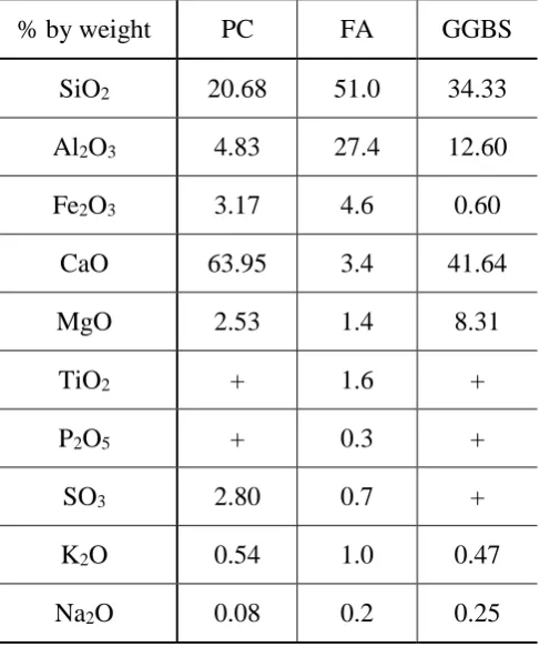
Table 2. Oxide analysis of materials used in experimental programme (+ = not determined)

% by weight PC FA GGBS

SiO2 20.68 51.0 34.33

Al2O3 4.83 27.4 12.60

Fe2O3 3.17 4.6 0.60

CaO 63.95 3.4 41.64

MgO 2.53 1.4 8.31

TiO2 + 1.6 +

P2O5 + 0.3 +

SO3 2.80 0.7 +

K2O 0.54 1.0 0.47

Table 3. Averaged concrete conductivity at 28-days 28) after casting based on

electrode-pair measurements within the surface 7.5cm (2-point) and 4-point measurements at 7.5cm.

(The number in brackets is the standard deviation for results).

Mix w/b ratio

2-point

28

(×10-4 S/cm)

4-point

28

(×10-4 S/cm)

PC

0.35 1.38 (0.14) 1.40 (0.11)

0.65 2.72 (0.23) 3.09(0.21)

FA/35

0.35 1.05 (0.05) 1.12 (0.09)

0.65 2.54 (0.20) 2.66 (0.15)

GGBS/65

0.35 0.31 (0.20) 0.32 (0.02)

0.65 0.59 (0.04) 0.69 (0.04)

Table 4. Equivalent conductivity at infinite dilution and conductivity coefficients for Na+,

K+ and OH- ions at 25ºC.

Species o _(cm2 _{S/mol) G (mol/L)}-½

Na+ 50.1 0.733

K+ 73.5 0.548

Table 5. Computed formation factors (F) for the concrete mixes in Table 1 at 28-days (F28)

and 180-days (F180) after casting (75% degree of hydration assumed throughout).

Mix Ref: PC FA/35 GGBS/65

w/b 0.35 0.65 0.35 0.65 0.35 0.65

p

(S/cm)

0.091 0.041 0.120 0.054 0.035 0.016

28

(×10-4 S/cm)

1.38 2.72 1.05 2.54 0.31 0.59



(×10-4 S/cm) 0.86 1.75 0.15 0.34 0.14 0.25

F28 659 151 1143 213 1129 271

FIGURE CAPTIONS

Figure 1. Embedded electrode array

Figure 2. Calibration curve for electrode array used in experimental programme (error bars

represent one standard deviation).

gure 3. Conductivity versus time response for electrodes positioned at 1.0, 2.0 and 7.5cm from

surface for PC concrete specimens (w/b = 0.65) undergoing cyclic ponding.

Figure 4. Decrease in conductivity during initial 28-days after casting for (a) w/b=0.35 and (b)

w/b=0.65.

Figure 5. Decrease in conductivity during 10-400 days after casting for (a) w/b = 0.35 and (b) w/b

= 0.65.

Figure 6. Curve-fits to conductivity versus time response based on 3 (three) measurement points at

10, 20 and 28-days for (a) w/b = 0.35 and (b) w/b = 0.65.

Figure 7. Calculated pore-water conductivity for the cementitious binders used within the

experimental programme for (a) PC, (b) FA/35 and (c) GGBS/65.

Figure 8. Estimated diffusion coefficient based on conductivity measurements for concrete, (a)

w/b = 0.35 and (b) w/b = 0.65.

Figure 1

Electrodes positioned at 7.5cm from surface for 2-point and 4-point

measurements

Figure 2

0.005 0.01 0.02 0.05 0.1 0.2

0.02 0.05 0.1 0.2 0.5

PC: w/b=0.35 PC: w/b=0.65 GGBS/65: w/b=0.35 GGBS/65: w/b=0.65 FA/35: w/b=0.35 FA/35: w/b=0.65

1/R_conc (10-3 S) con

c

(



1

0

-3 S

/c

m

Figure 3

0 0.5 1.0 1.5 2.0 2.5

100 150 200 250 300

10 mm 20 mm 75 mm PC: w/b=0.65

Time, t (days) t

(



1

0

-4 S

/c

m

Figure 4 0 5 10 15 20

0 10 20 30

PC FA/35 GGBS/65 (b) w/b = 0.65

Time, t (days) t (  1 0 -4 S /c m ) 0 2 4 6 8 10

0 10 20 30

PC FA/35 GGBS/65 (a) w/b = 0.35

Time, t (days)

 t (  1 0

-4 S

/c

m

Figure 5

0 1 2 3

0 50 100 150 200 250 300 350 400

PC [_t = 1.3810-4(28/t) 0.26] FA/35 [_t = 1.0510-4(28/t)0.99] GGBS/65 [t = 0.3110

-4 (28/t)0.45] (a) w/b = 0.35

Time, t (days)

t (  1 0 -4 S /c m ) 0 1 2 3 4 5 6

0 50 100 150 200 250 300 350 400

PC [t = 2.7210 -4

(28/t)0.25] FA/35 [t = 2.540

-4 (28/t)0.94] GGBS/65 [t = 0.5910

-4 (28/t)0.46] (b) w/b = 0.65

Time, t (days)

Figure 6 0

1 2 3

0 50 100 150 200 250 300 350 400

PC [_t = 1.3810-4(28/t)0.22 ]

FA/35 [

t = 1.0510

-4

(28/t)0.87 ]

GGBS/65 [_t = 0.3110-4(28/t)0.53 ]

(a) w/b = 0.35

Time, t (days)

t (  1 0 -4 S /c m ) 0 1 2 3 4 5 6

0 50 100 150 200 250 300 350 400

PC [

t = 2.7210

-4

(28/t)0.20 ]

FA/35 [_t = 2.5410-4(28/t)0.72 ]

GGBS/65 [

t = 0.5910

-4

(28/t)0.68 ]

(b) w/b = 0.65

Time, t (days)

Figure 7

0 0.05 0.10 0.15

40 50 60 70 80 90 100

w/b = 0.35 w/b = 0.65 (a) PC

Degree of hydration (%) p (S /c m ) 0 0.05 0.10 0.15

40 50 60 70 80 90 100

w/b = 0.35 w/b = 0.65 (b) FA/35

Degree of Hydration (%) p ( S /c m ) 0 0.01 0.02 0.03 0.04 0.05

40 50 60 70 80 90 100

w/b = 0.35 w/b = 0.65 (c) GGBS/65

Figure 8 0.1 0.2 0.5 1 2 5

10 20 50 100 200

FA/35 GGBS/65

(a) w/b = 0.35

PC

Time, t (days)

Di (  1 0 -1

2 m 2 /s ) 1 2 5 10 20

10 20 50 100 200

(b) w/b = 0.65 FA/35 GGBS/65 PC

Time, t (days)

Di (  1 0 -1

2 m 2 /s

Figure 9 Di

Time

tex t

Deff