Can weakly nonlinear theory explain Faraday wave patterns near onset?

This is a repository copy of

Can weakly nonlinear theory explain Faraday wave patterns

near onset?

.

White Rose Research Online URL for this paper:

http://eprints.whiterose.ac.uk/89783/

Version: Accepted Version

Article:

Skeldon, AC and Rucklidge, AM (2015) Can weakly nonlinear theory explain Faraday

wave patterns near onset? Journal of Fluid Mechanics, 777. 604 - 632. ISSN 0022-1120

https://doi.org/10.1017/jfm.2015.388

[email protected] https://eprints.whiterose.ac.uk/ Reuse

Unless indicated otherwise, fulltext items are protected by copyright with all rights reserved. The copyright exception in section 29 of the Copyright, Designs and Patents Act 1988 allows the making of a single copy solely for the purpose of non-commercial research or private study within the limits of fair dealing. The publisher or other rights-holder may allow further reproduction and re-use of this version - refer to the White Rose Research Online record for this item. Where records identify the publisher as the copyright holder, users can verify any specific terms of use on the publisher’s website.

Takedown

If you consider content in White Rose Research Online to be in breach of UK law, please notify us by

Can weakly nonlinear theory explain

Faraday wave patterns near onset?

A. C. S K E L D O N

_†

_{, and A. M. R U C K L I D G E}

1

Department of Mathematics, University of Surrey, Guildford, Surrey, GU2 7XH, UK 2

Department of Mathematics, University of Leeds, Leeds, LS2 9JT, UK

(Received ?; revised ?; accepted ?. - To be entered by editorial office)

The Faraday problem is an important pattern-forming system that provides some middle ground between systems where the initial instability involves just a single mode and in which complexity then results from mode interactions or secondary bifurcations, and cases where a system is highly turbulent and many spatial and temporal modes are excited. It has been a rich source of novel patterns and of theoretical work aimed at understanding how and why such patterns occur. Yet it is particularly challenging to tie theory to experiment: the experiments are difficult to perform; the parameter regime of interest (large box, moderate viscosity) along with the technical difficulties of solving the free boundary Navier–Stokes equations make numerical solution of the problem hard; and the fact that the instabilities result in an entire circle of unstable wavevectors presents considerable theoretical difficulties.

In principle, weakly nonlinear theory should be able to predict which patterns are stable near pattern onset. In this paper we present the first quantitative comparison between weakly nonlinear theory of the full Navier–Stokes equations and (previously published) experimental results for the Faraday problem with multiple frequency forcing. We confirm that three-wave interactions sit at the heart of why complex patterns are stablised but also highlight some discrepancies between theory and experiment. These suggest the need for further experimental and theoretical work to fully investigate the issues of pattern bistability and the role of bicritical/tricritical points in determining bifurcation structure.

Key words:Faraday waves, superlattice patterns, quasipatterns

1. Introduction

Since Faraday (1831) identified that regular patterns can appear on the surface of a shaken container of fluid, the Faraday experiment has been an important system for investigating pattern formation. Experiments in the 1980’s such as those conducted by Simonelli & Gollub (1989) tended to focus on the dynamics of the interaction of patterns in small containers excited by a sinusoidal forcing with a single frequency component. More recently the focus has switched to larger containers with multiple frequency com-ponents: as pointed out in Arbell & Fineberg (1998), one special feature of the Faraday experiment is that by using multiple frequency forcing one can investigate the interac-tion of a small number of controllable modes with different characteristic length scales. This provides some middle ground between pattern-forming systems where the initial instability involves just a single mode and in which complexity then results from sec-ondary bifurcations, such as in the B´enard–Marangoni experiment or the Taylor-Couette

† Email address for correspondence: [email protected]

2 A. C. Skeldon and A. M. Rucklidge

experiment, and cases where a system is highly turbulent and many spatial and temporal modes are excited.

Within the Faraday experiment, a rich variety of complex patterns are seen, some of which have a complicated spatial structure but are time-periodic with the periodicity of the drive and some with both a complicated spatial and temporal structure. Aside from the ubiquitous stripes, squares and hexagons, observed patterns include: quasipat-terns (Christiansenet al.(1992), Edwards & Fauve (1994)); superlattice patterns (SL1) (Kudrolliet al. (1998); Epstein & Fineberg (2006)); spatially subharmonic superlattice states, modulated hexagonal disorder, two mode superlattices and unlocked states (Ar-bell & Fineberg (1998)); oscillons (Ar(Ar-bell & Fineberg (2000)), and double hexagon states Arbell & Fineberg (1998). An excellent summary of many of the experimental results is given in Arbell & Fineberg (2002).

In parallel with the experiments, theoretical advances have resulted in an effective nu-merical method for performing the linear stability analysis of the Navier–Stokes equation that marks the transition from an unpatterned to patterned state (Kumar & Tuckerman (1994)). The challenge here is that many of the experiments are carried out at moderate viscosity whereas early theoretical results of Benjamin & Ursell (1954), which help ex-plain the underlying instability mechanism, are for an inviscid fluid. There have also been theoretical explanations for why, unlike the B´enard–Marangoni system, the observed pat-terned states include superlattice patterns (Silber & Skeldon (1999); Silberet al.(2000); Silber & Proctor (1998); Rucklidge & Silber (2009)).

These theoretical mechanisms rely on three-wave resonance between critical modes and modes close to critical and have successfully explained why particular superlattice patterns are observed. The suggested theoretical mechanism for the appearance of super-lattice patterns is compelling, and the link between which modes are excited and which patterns are observed has been explored in some detail experimentally, for example see Arbell & Fineberg (2002); Epstein & Fineberg (2006). However, without carrying out a careful quantitative comparison between experiment and theory, it is hard to know the extent to which the theoretical ideas really do explain the experimental results (Boden-schatz et al.(2000)). This is particularly true for the Faraday experiment where, as we will explain in greater detail below, the very region for which the theory predicts super-lattice patterns is the region for which some of the underlying assumptions of the theory break down.

While it is not possible to write down closed-form solutions of the full Navier–Stokes equations for the Faraday problem, quantitative predictions of the patterns expected near the transition from non-patterned to pattern states can be made using weakly nonlinear analysis (Skeldon & Guidoboni (2007)). Weakly nonlinear analysis centres on using an asymptotic expansion in terms of the slowly varying amplitudes of the critical modes at onset, using ideas first developed in Malkus & Veronis (1958) and Segel & Stuart (1962) in the context of convection experiments. Analysis of the resulting amplitude equations leads to predictions on the relative stability of different patterned states.

gravitational and surface tension forces. Results from this theoretical study agree very well with the author’s experimental results. However, the extension to multiple frequency forcing is far from trivial. The method used by Chen & Vi˜nals (1999) to reduce the Navier-Stokes equations to amplitude equations is not applicable, and the more general theory in Skeldon & Guidoboni (2007) is needed; the addition of more frequency components introduces more non-dimensional parameters, resulting in a much greater ability to probe underlying three-wave mechanisms. Consequently, patterns such as superlattice patterns, which are not observed in the single frequency context, are found. In fact, as we will show, for multiple frequency excitation there remain many open questions. We note also that Westraet al.(2003) use a Lyapunov stability argument to determine preferred patterns. We use similar arguments, but have in addition carried out a bifurcation analysis of the relevant amplitude equations. This has the added benefit of not only determining the ‘most stable’ pattern but also indicating regions where patterns are bistable.

Specifically, in this paper we discuss to what extent the existing weakly nonlinear the-ory can explain observed patterns in multiple-frequency Faraday experiments and provide some new explanations in some cases. While agreement is very good in many cases, we note that quantitatively linking theory with experiment is particularly challenging after-the-fact as the results are sensitive to precise values of viscosity and surface tension and even the sign of the drive term, something that is not normally recorded. There are also places where the analysis strongly suggests that patterns should have a subharmonic component, when no subharmonic component has been observed. In particular, with re-gard to the superlattice patterns, we discuss two methods that have been used to promote the stability of superlattice patterns: firstly by approaching the so-called bicritical point in two-frequency forced experiments; and, secondly, by adding a third frequency to the drive. We highlight the differences between these two mechanisms.

Overall, we confirm that three-wave interactions sit at the heart of why complex pat-terns are stablised. However, the discrepancies between theory and experiment suggest the need for further experimental and theoretical work to fully investigate the issues of pattern bistability and the role of bicritical/tricritical points in determining bifurcation structure.

2. Equations

Using a variety of container shapes, Edwards & Fauve (1994) elegantly demonstrated that many of the patterns that occur with moderate viscosity fluids in large containers are not strongly dependent on the lateral boundaries of the container. Consequently it is a reasonable modelling assumption to consider an infinite horizontal layer of viscous incompressible fluid of finite depth that is subjected to gravity ˜gand to a vertical periodic excitation with non-dimensional frequency components jω. At the lower boundary the fluid is in contact with a rigid plane while at the upper boundary the surface is open to the atmosphere. This means that the upper surface is a free boundary whose shape and evolution is an unknown of the problem.

4 A. C. Skeldon and A. M. Rucklidge incompressible Navier–Stokes equations

∇ ·u= 0,

∂tu+u· ∇u=−∇P+C∆u−(1 +f(t))e3, (2.1)

where u = (u, v, w) is the velocity field, P the pressure and for multiple frequency excitation,

f(t) =X j

ajcos(jωt+φj), (2.2)

wherej are integers and the non-dimensional amplitudesaj and phasesφj are real. It is assumed that the bottom of the container is rigid so that atz =−˜h/˜l the fluid satisfies the no-slip boundary conditions

u=v=w= 0. (2.3)

At the free surfacez =ζ(x, y;t) we have the kinematic condition, which says that the surface is advected by the fluid, and two further conditions, one for the balance of the tan-gential stresses and one for the balance of normal stresses. This leads to three conditions atz=ζ(x, y;t) namely

∂tζ+u∂xζ+v∂yζ=w,

t1·Tn=t2·Tn= 0, (2.4)

−P+ 2CnD(u)n=BH −pe,

where T= −PI+ 2CD(u) is the stress tensor, D(u) = (∇u+∇T_{u)/2 is the} rate-of-strain tensor, and H =∇H ·(∇Hζ/

p

1 +|∇Hζ|2) is the double mean curvature. Note that∇= (∇H, ∂z) and∇H = (∂x, ∂y). The unit normal and tangent vectors are defined as

n(x, y;t) = −p ∂xζ

1 +|∇Hζ|2

,−p ∂yζ

1 +|∇Hζ|2

,p 1

1 +|∇Hζ|2

!

,

t1(x, y;t) =

1

p

1 +|∂xζ|2

,0,p ∂xζ

1 +|∂xζ|2

!

,

t2(x, y;t) = 0,

1

p

1 +|∂yζ|2

,p ∂yζ

1 +|∂yζ|2

!

,

The units of length, time, velocity and pressure have been taken as ˜l,

q

˜ l/˜g,

q

˜

g˜land ˜̺g˜˜l respectively, where, ˜̺is the density of the fluid and ˜g is the acceleration due to gravity. The length scale ˜lis taken to be a length scale that is typical for the problem, such as the primary wavelength of the observed patterns. Here,peis the dimensionless pressure of the external ambient fluid and is assumed known. There are two non-dimensional parameters associated with the fluid, namely:C= ˜ν/(˜g˜l3

)1/2

, the square of the inverse of the Galileo number, andB = ˜σ/̺˜g˜˜l2

z= 0

z=−˜h/˜l

z=ζ(x, y;t)

˜

g

f(t)

Figure 1.Sketch of a cross-section through the layer of fluid.

As in Kumar & Tuckerman (1994), it is convenient to define a new pressure,

p=P+ (1 +f(t))z, (2.5)

which has the effect of shifting the acceleration term from the momentum equation to the normal stress condition. In addition, we eliminate the pressure from the momentum equation by taking−(∇ × ∇×). Using the relation∇ × ∇ ×u=∇(∇ ·u)−∆uand the fact that∇ ·u= 0, the problem then becomes

∇ ·u= 0,

∂t∆u−C∆∆u=∇ × ∇ ×(u· ∇u), (2.6)

with boundary conditions onz=−˜h/˜l,

u=v=w= 0 (2.7)

and onz=ζ,

∂tζ+u∂xζ+v∂yζ=w,

t1·Tn=t2·Tn= 0, (2.8)

2CnD(u)n=BH+p−pe−(1 +f(t))ζ.

Equations (2.6) with boundary conditions (2.7) and (2.8) have a trivial solution,

u=0, p=pe, ζ= 0. (2.9)

This solution corresponds to an unpatterned state where there is no relative motion of the fluid with respect to the moving frame so the surface of the fluid is flat.

3. Does linear theory agree with experiments?

6 A. C. Skeldon and A. M. Rucklidge

Benjamin & Ursell (1954) recognised that the linear stability of the flat-surface solution for an inviscid, infinite depth fluid driven by a single frequency reduces to a Mathieu equation. The Mathieu equation contains two parameters, related to the frequency ˜ωand amplitude ˜aof the excitation respectively. Solutions to the Mathieu equation divide the parameter plane into regions of bounded and regions of unbounded solutions where the regions of unbounded solutions form tongues that touch the frequency axis at frequencies mω/˜ 2, m = 1,2..., the largest tongue occuring for m = 1. The tongues are typically classified as either harmonic or subharmonic, depending on whether or not they are an integer multiple of the frequency ˜ω. This picture is modified with the addition of damping: the boundaries of the regions are perturbed and no longer touch the frequency axis, consequently a finite amplitude of excitation is required to excite waves; the regions of bounded solutions become regions where the unpatterned state is locally stable; the unbounded regions become regions where the unpatterned state is unstable.

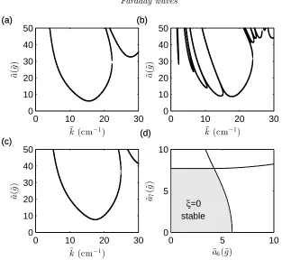
Kumar & Tuckerman (1994) identified a numerical method to find the instability tongues that can be used for all fluid viscosities and all depths and applied it to the case of single frequency excitation. This was extended to multiple frequency excitation by Besson et al. (1996). A typical example of tongues computed using Besson et al. (1996)’s method and the corresponding bifurcation set for the primary stability bound-ary is shown in figure 2.

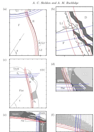
The linear stability problem appears to be solved: the numerical method works well and in Bessonet al.(1996) the authors show that there is excellent agreement between their linear stability calculations and experiments. However, unless experiments and theory are carried out hand-in-hand, in practice there remain some difficulties in obtaining really good agreement between theory and experiment even for this first transition from patterned to unpatterned state. This is illustrated in figure 3 where numerical linear stability results are superimposed on the experimental bifurcation sets published in: Edwards & Fauve (1994) (panels (a) and (b)); Kudrolliet al.(1998) (panel (c)); Epstein & Fineberg (2006) (panel (d)), and Ding & Umbanhowar (2006) (panels (e) and (f)).

The central issue here is that the position of the curves is sensitive to the values of the surface tension, density and the viscosity and yet the values quoted in papers are often taken from the manufacturers’ specifications for the fluids used. In order to illustrate the issue, in each case we have plotted the linear stability curves for the quoted viscosity and the quoted viscosity plus or minus 5%, a typical quoted tolerance for the viscosity value. From figure 3 we see that: for the experiments in Edwards & Fauve (1994) and Ding & Umbanhowar (2006), the upper extreme for the viscosity fits the data best (panels (a),(b),(e) and (f)); for those in Kudrolli et al. (1998), the lower extreme fits the subharmonic boundary best, but not the harmonic boundary (panel (c)); for the experiments in Epstein & Fineberg (2006) the linear stability analysis suggests that the actual viscosity of the fluid was higher than the upper value (panel (d)). We have focussed here on viscosity because for the different fluids used in the results presented here, errors in the viscosity have the biggest effect on the linear stability boundary. An error in the viscosity of 5% can result in an error in the linear stability boundary of 5%, whereas a 5% error in either the surface tension or the density leading to a 5% error in the ratio ˜σ/̺˜leads to an error in the linear stability boundary of only around 1%.

0 10 20 30 0 10 20 30 40 50 ˜

k(cm−1)

˜a (˜ g ) (a) (a)

0 10 20 30

0 10 20 30 40 50 ˜

k(cm−1)

˜a (˜ g ) (b) (b)

0 10 20 30

0 10 20 30 40 50 ˜

k(cm−1₎

˜a (˜ g ) (c) (c)

0 5 10

0 5 10 (d)

˜

a₆(˜g)

˜a7 (˜ g ) ξ=0 stable (d) ξ=0 stable

Figure 2.Typical tongues and linear stability region for the unpatterned state computed using the method of Bessonet al.(1996). Parameters as for Kudrolliet al.(1998): the (dimensional) excitation is ˜f(˜t) = ˜a6cos 6˜ωt˜+ ˜a7cos(7˜ω˜t+φ7), where ˜a6 = ˜acosχ, ˜a7 = ˜asinχ,φ7 = 20◦, ˜

ω/2π= 16.44 Hz, ˜σ = 20.6 dyn cm−1

, ˜ν = 0.20 cm2 s−1

, ˜̺= 0.95 g cm−3

, ˜h= 0.3 cm. Note that the structure inherited from the Mathieu equation is seen by the fact that the minimum of each tongue occurs at half integer multiples of the drive frequency. In (a)χ= 0◦_{, the forcing}

reduces to ˜f(˜t) = ˜a6cos 6˜ωt˜, with a forcing frequency of 6˜ω. The largest tongue has a minimum for wavenumber of approx 15cm−1

for a forcing amplitude ˜a of approx 7.5˜gand corresponds to a mode of frequency 6 ˜ω

2 . In (c), χ = 90

◦ _{the forcing reduces to ˜f(˜t) = ˜a}

7cos 7˜ω˜t with a forcing frequency of 7˜ωleading to a primary instability mode with frequency 7˜ω/2. In the case of (b), χ = 63◦_{, the presence of both 6˜ω and 7˜ω components in the forcing frequency mean}

that the drive has periodicity 2π/ω˜ and is therefore of frequency ˜ω. This leads to tongues at

mω/˜ 2. . . , m= 1,2, . . .. The first five tongues that are visible from left to right correspond to: ˜

ω/2,4˜ω/2,5˜ω/2,6˜ω/2,7˜ω/2. The largest tongues correspond to the 6˜ω/2 and the 7˜ω/2 modes and are driven by the two main frequency components of the drive. There are tongues corre-sponding to modes with frequency 2˜ω/2 and 3˜ω/2 but these occur off the top of the region shown. This particular value ofχis close to the ‘bi-critical’ point where both harmonic modes with frequency 6˜ω/2 and sub-harmonic modes with frequency 7˜ω/2 onset simultaneously. It is close to this bi-critical point that many of the exotic patterns are observed. (d) Bifurcation set showing the position of the tongue minimum that marks the instability of the unpatterned state, as a function of ˜a6and ˜a7.

4. Predicting patterns close to onset

4.1. Theoretical ideas

8 A. C. Skeldon and A. M. Rucklidge

(a) (b)

(c)

(d)

(e) (f)

Figure 3. Comparison of the experimentally measured transition from unpatterned to pat-terned state with numerically calculated linear stability curves using the method of Besson et al.(1996). For each of the numerical calculations, three different values for the viscosity are used. (a) and (b) Numerical curves overlaid on figure 12 of Edwards & Fauve (1994). Adapted with permission from Edwards & Fauve (1994). ˜σ= 65 dyn cm−1

; ˜ν = 1.00±0.05 cm2 s−1

; ˜

̺= 1.22 g m−3

; ˜h= 0.29 cm; ˜aj, j={4,5};φ4 = 0;φ5 = 75◦; ˜ω/2π= 14.6 Hz. (c) Numerical curves overlaid on figure 6(a) of Kudrolliet al.(1998) reprinted from Physica D, Vol 123, A. Kudrolli, B. Pier and J.P. Gollub, ‘Superlattice patterns in surface waves’, p99–111, Copyright (1998), with permission from Elsevier. ˜σ= 20.6 dyn cm−1

; ˜ν= 0.20±0.01 cm2 s−1

; ˜̺= 0.95 g m−3

; ˜h= 0.3 cm; ˜aj, j={4,5};φ4= 0;φ5= 16◦; ˜ω/2π= 22 Hz. (d) Numerical curves overlaid on figure 2 of Epstein & Fineberg (2006). Adapted with permission from Epstein & Fineberg (2006). Copyrighted by the American Physical Society. ˜σ= 20.6 dyn cm−1

; ˜ν= 0.180±0.009 cm2

s−1

; ˜̺= 0.949 g m−3

; ˜h = 0.3 cm; ˜aj, j ={6,7}; φj = 0◦; ˜ω/2π = 14 Hz. (e) and (f) Numerical curves overlaid on figures 1 and 3(a) of Ding & Umbanhowar (2006). Adapted with permission from Ding & Umbanhowar (2006). Copyrighted by the American Physical Society. ˜

σ = 20.6 dyn cm−1

; ˜ν = 0.20±0.01 cm2 s−1

; ˜̺ = 0.95 g m−3

; ˜h = 0.65 cm; ˜aj, j ={4,5};

(a)

k2 k1

k3

60◦

(b)

k2

k1

k3

θ

(c)

k1

k2

k3

θ

(d)

k1

k2

k3

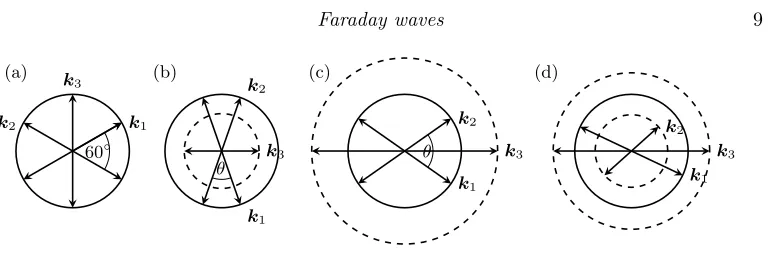
Figure 4.Possible spatial three-wave resonant interactions defined such thatk1+k2=k3. (a)|k1|=|k2|=|k3|; (b)|k1|=|k2|>|k3|; (c)|k1|=|k2|<|k3|; (d)|k1| 6=|k2| 6=|k3|.

the same wave number but different orientations often lead to the observation of patterns with, for example, hexagonal symmetry. In principle, superlattice patterns could also occur in convection experiments (Skeldon & Silber (1998)), but in practice they have not been seen without the addition of a vertical oscillation, as in Rogerset al. (2000).

The ubiquitous occurrence of hexagons is a consequence of the importance of three-wave interactions in determining which patterned states occur: three-three-wave interactions give rise to the lowest order nonlinear (quadratic) terms in the amplitude equations that describe behaviour close to onset. For B´enard–Marangoni convection, where instability to a single dominant wavenumber occurs, the three-wave interaction of importance occurs between three wave vectors with the same critical wavenumber, as shown in figure 4(a). A distinct feature of the Faraday problem is that the Mathieu tongue-like structure to the linear stability problem means that although typically there is a single mode that becomes unstable first, there are nearby modes with different wavenumbers that are only weakly damped. This can give rise to other three-wave interactions of relevance, such as those shown in figure 4(b), (c) and (d).

These three-wave interactions involve waves with wavevectors k1,k2 and k3 and re-spective frequenciesnω/2, pω/2 andqω. For the three waves to interact they must satisfy a spatial resonance condition,

±k1±k2=k3, (4.1)

and a temporal resonance condition. In the spatial resonance condition the choice of sign arises because the waves are standing waves and so have spatial fourier components with both signs of wave vector. The temporal resonance condition depends on both the frequencies of the waves and the various frequencies contained within the forcing term f(t) and requires

±n 2 ±

p

2 ±j=q (4.2)

wherej is one of the frequency components of the drive see equation (2.2),cf Topazet al. (2004) and where all possible sign combinations of the different terms on the left-hand side need to be considered because the waves are standing waves and the forcing is real. The fact that a temporal resonance condition needs to be satisfied is one feature that distinguishes the Faraday problem from Swift–Hohenberg multiple resonance problems such as those studied in M¨uller (1994), Lifshitz & Petrich (1997), Rucklidgeet al.(2012) and others. This means that results from Swift–Hohenberg-like equations need to be interpreted with care when applied to the Faraday problem, a point that we will return to in the discussion.

10 A. C. Skeldon and A. M. Rucklidge

modes ki as shown in figure 4(b) or (c) with amplitudes Ai, then using a multiple timescale expansion near onset would lead to equations for the evolution of the amplitudes on a slow timescale of the form

˙

A1=λ1A1+α1A2A3+A1(a|A1| 2

+b0|A2| 2

+c|A3| 2

) +. . . ˙

A2=λ1A2+α1A1A3+A2(b0|A1|2+a|A2|2+c|A3|2) +. . . (4.3)

˙

A3=λ2A3+α2A1A2+A3(d|A1| 2

+d|A2| 2

+e|A3| 2

) +. . . ,

whereλ1andλ2are the linear growth rates of the respective modes, andα1, α2, a, b0, c, d

and e are all real-valued constants. The quadratic coefficients,α1 and α2 are non-zero

only if the temporal resonance condition is met. Note that there is no assumption of weak forcing/damping and so terms such asA1 do not appear (Alnahdiet al.(2014)).

Now, the mode with wavevectork3 is not at its critical point but is weakly damped, soλ2<0 and, close to onset (i.e.|λ1|small enough), it is therefore slaved by the critical

modes. Consequently, one can perform a centre manifold reduction on equations (4.3), resulting in

A3=−

α2

λ2

A1A2+. . . ,

and

˙

A1=λ1A1+A1(a|A1|2+b(θres)|A2|2) +. . .

˙

A2=λ1A2+A2(b(θres)|A1| 2

+a|A2| 2

) +. . . , (4.4)

where

b(θres) =b0+bres, bres=−

α1α2

λ2

. (4.5)

The presence of the weakly damped mode therefore changes the value of the cross-coupling coefficient b(θres) between modes with wavevectors k1 and k2, offset at an

angle θres. The value of θres is determined by the ratio of critical and weakly damped

wavenumbers, but the same idea holds for any three-wave interaction between any k1

andk2on the critical circle. This results in a functionb(θ) with either a distinctive peak or dip at θ=θres, depending on the sign of α1α2 and on the weakness of the damping

for the weakly damped mode.

Analysing the amplitude equations (4.4) shows that there are two types of solutions that bifurcate from the trivial solution A1 = A2 = 0, namely stripes (A1 6= 0, A2 = 0

or vice versa) and rectangles (A1 = A2). The relative stability of rectangles to stripe

perturbations is dependent on the relative size of the self-coupling coefficientain equation (4.4) andb(θres) where, ifbres>0 (α1α2>0), then the stability of rectangles is enhanced

by the three-wave interaction and ifbres<0 (α1α2<0), then the stability of rectangles

is suppressed.

Of course, in the Faraday problem there are not just two modes and there are many interactions and several weakly damped circles, but this idea that three-wave resonances can promote patterns associated with the angleθresis powerful (Silberet al.(2000)). The

The superlattice patterns observed by Kudrolliet al. (1998) for {6,7} excitation ex-emplify the idea and motivated the early theoretical work. The superlattice patterns that they observe are spatially periodic and a spatial Fourier transform of the pattern indicates that they consist of essentially two sets of hexagonal modes offset by an angle of 22◦_{. In this case, the particular three-wave resonance of relevance is of the type} illus-trated in figure 4(b) and is between a harmonic mode that is weakly damped of frequency 2˜ω/2, related to the 2˜ω/2 tongue, and two wavevectors with wavenumbers corresponding to the 6˜ω/2 tongue (Silber et al. (2000)). This was surprising because the superlattice state appears near the bicritical point where both 6˜ω/2 and 7˜ω/2 onset simultaneously and naively, from inspection of the linear stability diagram (see figure 2(b)) one would assume that it was a result of the interaction of 6˜ω/2 and 7˜ω/2 modes—the 2˜ω/2 tongue onsets at an amplitude of approximately 50 so is not even visible on the scale shown.

This argument not only explains the presence of the 22◦ _{superlattice patterns but also} why patterns with angles close to 30◦_{are seen inj={4,5}forcing (Skeldon & Guidoboni} (2007)). Extensions of this basic idea have been used to suggest ways to design forcing frequencies to promote particular patterns in both Faraday waves (Porteret al.(2004)) and in a model partial differential equation (Rucklidge & Silber (2009)).

The results of Kudrolliet al. (1998) and the theoretical results of Silberet al. (2000) showed how modes visible in the spatial Fourier transform of the experimentally ob-served pattern can be linked to critical/weakly damped modes and three-wave resonant interactions. It follows that given an experimentally observed pattern it should be pos-sible to confirm whether or not it is a result of a particular interaction by establishing which modes are present in the pattern. However, identifying precisely which modes are involved can be tricky, as we illustrate in the following section.

4.2. Practical identification of relevent modes

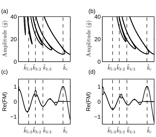
In Epstein & Fineberg (2006) a detailed comparison of different patterns, referred to as ‘grid’ states and labelled as 3 : 2, 4 : 3 and 5 : 3 respectively is presented. The spatial Fourier transform of the patterns enables the identification of the wavenumbers that are present in these patterns: in each case they appear to be dominated by modes sitting on two different circles, one on the primary harmonic instability with wavenumber ˜kc and a second circle with respective wavenumbers ˜k3:2= 0.38˜kc,˜k4:3= 0.55˜kcand ˜k5:3= 0.23˜kc. These ratios are fixed by the fact that the observed grid states consist of modes that fit on to a hexagonal lattice. This suggests that they are strong candidates for superlattice patterns that occur as a result of the mechanism discussed in section 4.1. Epstein & Fineberg (2006) computed the linear stability curves, and their linear stability diagrams are re-computed in figure 5(a) and (b). We note that the linear stability curves are similar, but not identical, to those given in Epstein & Fineberg (2006) particularly at small ˜k. This is because we have made a different choice in the sign of the forcing term to that made by Epstein & Fineberg (2006). This is explained further in Section 6. As stated by Epstein & Fineberg (2006) and, as can be seen in this figure, the ˜k3:2 wave number lines

up with the first harmonic tongue (2˜ω/2) and this strongly suggests that it is the same mechanism that produces the familiar 22◦ _{superlattice patterns, seen by Kudrolliet al.} (1998), that produces the ˜k3:2 grid state. For the two other states the situation is less

clear. Epstein & Fineberg (2006) state that ˜k4:3 lines up with the the second harmonic

tongue (4˜ω/2), but this is not clear from figure 5 (the position of the line drawn in figure 5 of Epstein & Fineberg (2006) is not consistent with the value of 0.55˜kc given). Epstein & Fineberg (2006) observe that the ˜k5:3 mode does not appear to be aligned with any

12 A. C. Skeldon and A. M. Rucklidge 0 20 40 A m p li tu d e (˜ g ) (a) ˜ kc ˜ k4:3 ˜ k3:2 ˜ k5:3 0 20 40 A m p li tu d e (˜ g ) ˜ kc ˜ k4:3 ˜ k3:2 ˜ k5:3 (b) −1 0 1 Re(FM) ˜ kc ˜ k_4:3 ˜ k_3:2 ˜ k_5:3 (c) −1 0 1 ˜ kc ˜ k_4:3 ˜ k_3:2 ˜ k_5:3 Re(FM) (d)

Figure 5. Linear stability curves and Floquet multipliers calculated from the finite depth Navier–Stokes equations (a) and (c) ˜h = 0.3 cm (b) and (d) ˜h = 0.2 cm. Parameter values are taken from Epstein & Fineberg (2006) and are ˜σ = 20.6 dyn cm−1

; ˜ν = 0.18 cm2 s−1

; ˜

̺= 0.949 g m−3

; ˜aj, j={6,7,2}, where ˜a6= 3.4,a˜7= 6.4,˜a2= 0.5;φj= 0◦; ˜ω/2π= 14Hz.

that emerges from the bicritical point, unlike the 3 : 2 and the 4 : 3 state that occur at a short distance from this point.

The difficulty here is that the linear stability diagram indicates that at an amplitude of excitation of approximately 7.5˜g the mode with wavenumber ˜kc and frequency 6˜ω/2 becomes unstable and that there are five other damped modes with smaller wavenumber. But the position of the tongues for these modes only gives a rough idea of the precise wavenumber and damping associated with each mode at the pattern onset amplitude of 7.5˜g.

More accurate information on the damped modes can be obtained by calculating the most critical Floquet multipliers, as detailed in Appendix A. The results for the parameter values used by Epstein & Fineberg (2006) are shown in figure 5(c) and (d). We note that with either possible sign for the forcing, the Floquet multipliers look very similar. As identified by Epstein & Fineberg (2006), the ˜k3:2 mode is aligned with the harmonic

tongue associated with frequency 2˜ω/2 for ˜h = 0.3 cm, but not for ˜h = 0.2 cm and supports their observation that the k3:2 grid state will be seen for ˜h= 0.3 cm and not

for ˜h = 0.2 cm. The remaining two wavenumbers ˜k5:3 and ˜k4:3 are very close to the

subharmonic waves of frequencies ˜ω/2 and 3˜ω/2 respectively. This clarifies the issue that the ˜k5:3 mode in Epstein & Fineberg (2006) did not appear to align with any mode on

the linear stability graphs and strongly suggests that the ˜k4:3mode was mis-identified as

harmonic. However, it also presents a problem in that temporal constraints mean that it is not possible for two harmonic wavevectors to form a three-wave resonance with a single subharmonic wavevector. Consequently, α1 = α2 = 0 in equations (4.3), so the

Epstein & Fineberg (2006) point out that the ˜k5:3 case could be a result of a

three-wave resonance between modes with frequencies ˜ω/2,6˜ω/2 and 7˜ω/2 and this is strongly supported by our Floquet multiplier calculation and is a permitted resonance in that it satisfies both spatial and temporal constraints. Such a resonance appears to be consistent with the spatial Fourier transform in figure 3(c) of Epstein & Fineberg (2006) and is similar in structure to previous states identified in figure 20(c) of Arbell & Fineberg (2002) as 2MS states. This would make it a three-wave resonance of the form shown in figure 4 (d). This kind of resonance was discussed briefly by Porter & Silber (2002) and results in patterns that occur in a wedge that emerges from the bicritical point. This is consistent with the bifurcation sets shown by Epstein and Fineberg. The only remaining conundrum for this particular pattern is that Epstein and Fineberg state that, although all the evidence points to subharmonic modes being important, no subharmonic component was found.

5. Observed patterns near onset: theoretical bifurcation sets

compared with experiment

In spite of the difficulties in identifying modes, nevertheless, in experiments with dom-inant forcing frequencies j = {4,5} or j = {6,7} there is a coherent picture: in the {6,7}case, observed superlattice patterns near onset have an angle of 22◦_{; forj={4,5},} observed patterns near onset are quasipatterns with an angle of 30◦_{. Although there} are technical difficulties with considering quasipatterns in the same way as superlattice patterns (Rucklidge & Rucklidge (2003); Rucklidge & Silber (2009); Iooss & Rucklidge (2010)), nevertheless they appear to fit within the same framework with resonant in-teractions with weakly damped modes associated with 2˜ω/2 contributing to bres and explaining the appearance of the appropriate angle. The different angle seen in the{4,5} case as compared with the {6,7} case is because of differences in the wavenumbers of the interacting modes. In both cases, superlattice/quasipatterns are only seen near the bicritical point where the two modes driven by the two main components of the forcing onset simultaneously.

Here, we aim to carry out a careful comparison of the results of weakly nonlinear the-ory and experimental results to explore to what extent there is quantitative agreement between experiments and theory as the bicritical point is approached. We present results from the experiments of Ding & Umbanhowar (2006) because we have excellent agree-ment for the linear stability curves with ˜ν = 0.21 cm2 _s−1_{, as shown in figure 3(e) and}

(f), and this set of experiments includes the most comprehensive study of how multiple frequencies interact via the superlattice mechanism outlined above. Specifically, acknowl-edging the importance of the 2˜ω/2 tongue, Ding & Umbanhowar (2006) carry out a series of experiments that systematically explore the effect of adding a third frequency that pro-motes this mode.

14 A. C. Skeldon and A. M. Rucklidge

Figure j ˜aj, φj Parameters Figure from

varied Ding & Umbanhowar (2006) 6 {4,5} (φ4, φ5) = (0,16◦) ˜a4 and ˜a5 1

7 {4,5,2} a˜2= 0.8˜g, (φ4, φ5, φ2) = (0◦,16◦,32◦) a4 anda5 3 (b) 8 {4,5,2} a˜5= 5˜g, (φ4, φ5, φ2) = (0◦,5◦,32◦) ˜a4 and ˜a2 4 (a) 9 {4,5,2} (˜a4,˜a5,˜a2) = (3.8,5.8,0.8)g, φ4= 0◦ φ5 andφ2 4(b) 10 {6,7 (φ6, φ7) = (0◦,40◦) ˜a6 and ˜a7 2 11 {6,7,2} a˜7= 7˜g,(φ6, φ7, φ2) = (0◦,40◦,80◦) ˜a6 and ˜a2 6(a) 12 {6,7,2} (˜a6,a˜7,˜a2) = (5.2,7.8,0.6)˜g,φ6= 0◦ φ7 andφ2 6(b)

Table 1.Summary information for figures comparing weakly nonlinear analysis with the experiments of Ding & Umbanhowar (2006).

results in determining the stability of stripes to any perturbation of the same wavenum-ber; the stability of hexagons to (i) stripes arbitrarily close to any given orientation (ii), rectangles arbitrarily close to any given aspect ratio, (iii) to superlattice patterns of any angle; the stability of rectangles to (i) stripes of any orientation (ii) superlattice pat-terns on the same lattice; the stability of superlattice patpat-terns to hexagons, stripes or rectangles that are made up of a subset of the superlattice wavevectors.

Since the weakly nonlinear stability analysis indicates that for many parameter values there is more than one stable pattern, results are presented in two ways, first showing the regions of stability for individual patterns—only those that have some region of sta-bility are shown, and secondly showing the bifurcation set for the most stable state, as computed from the weakly nonlinear coefficients using the Lyapunov functional given in Skeldon & Guidoboni (2007). The most stable states are superimposed on the experi-mental results of Ding & Umbanhowar (2006). In the case of superlattice patterns, the resonant interactions mean that it is always the particular pattern associated withθres that has the largest region of stability and it is perturbations associated with this angle that first destabilise hexagons. Consequently where superlattice patterns are shown it is always the superlattice pattern associated withθres that is relevant.

Ding and Umbanhowar consider the two sets of frequency components most widely used by other experimental groups, namelyj={4,5}andj={6,7}and then systematically investigate the inclusion of a third mode, so considering the combinations j ={4,5,2} andj={6,7,2}. We have carried out the weakly nonlinear stability analysis for each of their parameter studies and the results are presented in figures 6-12 where the principle parameters considered and the corresponding figures in Ding & Umbanhowar (2006) are summarised in table 1.

In each case the weakly nonlinear results are superimposed on the experimental re-sults. The parameters have been chosen to match those quoted in the paper of Ding & Umbanhowar (2006) with the exception of the viscosity where, as seen in figure 3, the linear stability curves fitted best with a viscosity of ˜ν = 0.21 cm2_s−1_{rather than ˜ν= 0.20}

cm2_s−1_{quoted in their paper (or the value of ˜ν = 0.204 cm}2_s−1 _{quoted in Ding (2006)).}

5.1. Results for {4,5} and{4,5,2}

In figure 6 we see that the weakly nonlinear theory predicts bistability between squares and hexagons for low values of ˜a5, with squares losing stability as the bicritical point

is approached. There is good agreement between the point at which squares become unstable (approximately ˜a5 = 2.2˜g, figure 6(a)), and the transition between squares

0 2 4 6 8 0

2 4 6

˜

a5(˜g)

˜

a4

(˜

g

)

(a) (a)

0 2 4 6 8

0 2 4 6

˜

a5(˜g)

˜

a4

(˜

g

)

(b) (b)

0 2 4 6 8

0 2 4 6

˜

a5(˜g)

˜

a4

(˜

g

)

(c) (c)

Figure 6. Comparison with figure 1 from Ding & Umbanhowar (2006). ˜

aj = {4,5},(φ4, φ5) = (0,16◦),ω/˜ 2π = 20 Hz. The fluid parameters are as in the cap-tion to figure 3(e),(f) with ˜ν = 0.21 cm2

s−1

. (a)-(b) Stability regions for different planforms. (a) Stable squares in green; unstable squares in grey; (b) stable hexagons in blue; unstable hexagons in grey. Note that for ˜a5 >0, there are quadratic terms in the amplitude equations which mean that hexagons bifurcate transcritically. The unstable solutions that are produced in this transcritical bifurcation are stabilised in a saddle-node bifurcation, resulting in a small region of stable, subcritical hexagons. This region of stable subcritical hexagons is only visible on the scale of the figure close to the bicritical point. (c) ‘Most stable’ state using a Lyapunov energy argument: + squares; ∗ hexagons; quasipatterns. The theoretical results are overlaid on figure 1 from Ding & Umbanhowar (2006). Adapted with permission from Ding & Umbanhowar (2006). Copyrighted by the American Physical Society.

suggests that there is a region of bistability between hexagons and squares and that in this region hexagons and not squares, as seen in the experiment, are the most stable state. Of course, in this region, the particular pattern observed experimentally will depend to some extent on the way in which the experiments were carried out. For example, if the experimental procedure was to fix ˜a4 and to increase ˜a5 from zero in small steps, one

16 A. C. Skeldon and A. M. Rucklidge

4 5 6 7 8

3 4 5

˜

a5(˜g)

˜

a4

(˜

g

)

(a)

4 5 6 7 8

3 4 5

˜

a5(˜g)

˜

a4

(˜

g

)

(b)

4 5 6 7 8

3 4 5 (c)

˜

a5(˜g)

˜

a4

(˜

g

)

Figure 7. Comparison with Ding & Umbanhowar (2006) Figure 3(b),

j = {4,5,2},(φ4, φ5, φ2) = (0,16◦,32◦). (a)-(b) Stability regions for different planforms. (a) Stable hexagons in blue, unstable hexagons in grey; (b) stable quasipatterns in red, unstable quasipatterns in grey. Both quasipatterns and hexagons bifurcate transcritically and may be stabilised in a saddle-node bifurcation. This can result in stable subcritical quasipatterns/hexagons. (c) ‘Most stable’ planform using a Lyapunov energy argument superimposed on figure 3(b) from Ding & Umbanhowar (2006). Adapted with permission from Ding & Umbanhowar (2006). Copyrighted by the American Physical Society. ∗ hexagons; quasipatterns,• disordered states, where the coloured symbols are the theoretical results and the black symbols the experimental results. The red line is the linear instability curve for the harmonic 2˜ω/2 tongue. The black cross indicates the point at which the experiment shown in figure 9(c) was carried out.

In figure 7, we see that by adding in a forcing component that excites the 2˜ω/2 mode directly Ding & Umbanhowar (2006) showed that they could increase the region of quasi-patterns, to the extent that they become the first pattern observed after the unpatterned state becomes unstable. Our theoretical results for the same parameter values also show an enhanced region for the superlattice patterns—but not as enhanced as for the exper-iment. Two possible reasons for this are (i) the nearby presence of the bicritical point where both the 2˜ω/2 and the 4˜ω/2 tongue onset simultaneously which means that our weakly nonlinear calculations would need to be extended; (ii) the sensitivity of the results to phase. We discuss both of these in more detail below.

Figure 8 shows excellent agreement between the theoretical results and the experimen-tal results for the pattern at onset for increasing ˜a2, with agreement diminishing with

distance from onset.

0 0.2 0.4 0.6 0.8 3.6

4 4.4 4.8

˜

a2(˜g)

˜

a4

(˜

g

)

(a)

0 0.2 0.4 0.6 0.8

3.6 4 4.4 4.8

˜

a2(˜g)

˜

a4

(˜

g

)

(b)

0 0.2 0.4 0.6 0.8

3.6 4 4.4 4.8

˜

a2(˜g)

˜

a4

(˜

g

)

(c)

Figure 8. Comparison with Ding & Umbanhowar (2006) figure 4(a).

j={4,5,2},a˜5= 5˜g,(φ4, φ5, φ2) = (0,16◦,32◦).(a) and (b) stability regions for hexagons and quasipatterns respectively. Coloured symbols stable; grey unstable. Hexagons and quasipatterns both bifurcate from the unpatterned state at a transcritical bifurcation, where the unstable bifurcating branch changes direction at a saddle-node bifurcation. This leads to regions of stable hexagons and quasipatterns that are subcritical. (c) ‘Most stable’ planform:∗hexagons; quasipatterns, overlaid on figure 4(a) from Ding & Umbanhowar (2006). Adapted with permission from Ding & Umbanhowar (2006). Copyrighted by the American Physical Society. The coloured symbols are the theoretical results and the black symbols the experimental results. The black dots indicate disordered states. Note that the linear stability boundary for the 2˜ω/2 mode is just off this diagram, and is approximately parallel to thea4 axis through a value ofa2≈1. The bicritical point where the 2˜ω/2 and the 4˜ω/2 modes onset simultaneously occurs when (˜a2,˜a4) = (1.05,3.80)˜g.

18 A. C. Skeldon and A. M. Rucklidge

The agreement in figure 9 is surprising because the results correspond to a point with ˜

a4= 3.8˜g,˜a5= 5.9˜g and ˜a2= 0.8˜g, which according to the theory is close to a transition

from quasipatterns to hexagons in a region where both hexagons and quasipatterns are stable, whereas in the experiment it is firmly in the quasipattern region. (In order to help cross-reference between the two figures, a black cross has been marked on both figure 7(c) and figure 9.) Figure 9 highlights the sensitivity of the results to phase and in fact, with our weakly nonlinear analysis we find that the size of the region of quasipatterns changes significantly depending on the phase. This sensitivity to the precise value of the phase could be part of the difficulty in obtaining agreement for the onset of quasipatterns in figure 7.

The results are, of course, also sensitive to the viscosity. Away from the bicritical point, changing the viscosity tends to translate the nonlinear bifurcation lines as one might expect: upwards if the viscosity is increased, downwards if the viscosity is decreased, in line with the changes to the transition from unpatterned to patterned state seen in Figure 3. Close to the bi-critical point the effects are more pronounced with small changes in viscosity sometimes leading to large changes in the regions in which particular patterns dominate.

5.2. Results for {6,7} and{6,7,2}

In figure 10 the weakly nonlinear theory predicts bistability between squares and hexagons for low values of ˜a7, with squares losing stability as the bicritical point is approached. As

for figure 6, although there is good agreement between the point at which squares become unstable (approximately ˜a7= 4.5˜g), and the transition between squares and hexagons in

the experiment, this agrees less well with the results of the energy argument.

In figure 11 both theory and experiment agree that for low and moderate values of ˜a2

hexagons are the preferred pattern. As ˜a2increases, hexagons are replaced by superlattice

patterns, although the transition observed experimentally occurs slightly earlier than in the weakly nonlinear calculations. Away from onset, the agreement is qualitative rather than quantitative: in the experiments superlattice patterns are observed for a much larger region than predicted by the weakly nonlinear theory and hexagons are observed in regions where the theory predicts bistability of rectangles and hexagons, with rectangles being the most stable state. For large values of ˜a2and ˜a6, the experiments see disordered

states. The weakly nonlinear theory cannot predict such states, but note that none of the planforms considered are found to be stable for large ˜a2and ˜a6(there are no symbols

from the theoretical calculations in the top right of figure 11).

The results shown in figure 12 again show that the theoretical results have the same diagonal dependency as seen in the experiments, a consequence of a phase invariant as discussed further below. For the experimental results, white indicates a high correlation with the angle of 22◦_{and this does seem to align with where superlattice patterns occur,} although for much of the lighter regions the weakly nonlinear analysis predicts no stable pattern. The black regions correspond to a low correlation at 22◦ _{and Ding &} Umban-howar (2006) state that this region contains ‘disordered’ patterns: our theoretical results suggest that both rectangles and hexagons are stable for much of this region each having a similar Lyapunov energy. Consequently one might expect competition between these two states, resulting in the observed disorder.

5.3. Common themes From our comparison, a number of themes emerge:

φ₅

φ 2 (d)

0 π 2π

2π

π

0

0 π 2π

0 π 2π

φ₅

φ 2 (a)

0 π 2π

0 π 2π

φ₅

φ 2 (b)

0 π 2π

0 π 2π

φ₅

φ 2 (c)

Figure 9. Comparison with Ding & Umbanhowar (2006) figure 4(b). Phase diagram for j = {4,5,2} with (˜a4,˜a5,˜a2) = (3.8,5.8,0.8)˜g. (The position of this point for (φ5, φ2) = (16◦,32◦) is shown in figure 7(c).) (a)-(c) stability regions for squares, hexagons and quasipatterns respectively. Coloured symbols stable; grey unstable. (d) ‘Most stable’ plan-forms: + squares;∗hexagons;quasipatterns. The results are overlaid on figure 4(b) of Ding & Umbanhowar (2006). Adapted with permission from Ding & Umbanhowar (2006). Copyrighted by the American Physical Society. The cross indicates the point which corresponds to the cross in figure 7.

theory and experiment. The experimental results for the pattern at onset are consistent with the theory, but sometimes the pattern at onset is not that predicted by considering the Lyapunov argument. This is one difficulty in comparing with experimentpost festum, since in regions of bistability, which pattern is observed can depend on the way that the experiments are performed.

(c) When the additional forcing component (˜a2 6= 0) is included that promotes the

mode with frequency 2˜ω/2, then in both theory and experiments patterns associated with the resonant angle are promoted and consequently appear for a larger region of parameter space.

20 A. C. Skeldon and A. M. Rucklidge

0 2 4 6 8

0 2 4 6 8

˜

a7(˜g)

˜

a6

(˜

g

)

(a)

0 2 4 6 8

0 2 4 6 8

˜

a7(˜g)

˜

a6

(˜

g

)

(b)

0 2 4 6 8

0 2 4 6 8

˜

a7(˜g)

˜

a6

(˜

g

)

(c)

Figure 10. Comparison with Ding & Umbanhowar (2006), figure 2.

j = {6,7},(φ6, φ7) = (0,40◦),ω/˜ 2π = 16.5 Hz. (a)-(b) stability regions for rectangles and hexagons. Coloured symbols stable; grey unstable. (c) ‘Most stable’ planform: + rectangles;

0 0.2 0.4 0.6 0.8 5

5.5 6 6.5

˜

a2(˜g) ˜a6

(˜

g

)

(a)

0 0.2 0.4 0.6 0.8

˜

a2(˜g)

(b)

0 0.2 0.4 0.6 0.8

˜

a2(˜g)

(c)

0 0.2 0.4 0.6 0.8

5 5.5 6

˜

a2(˜g) ˜a6

(˜

g

)

(d)

Figure 11. Comparison with Ding & Umbanhowar (2006), figure 6(a).

j = {6,7,2},˜a7 = 7˜g,(φ6, φ7, φ2) = (0,40◦,80◦),ω/˜ 2π = 16.5 Hz. (a)-(c) stability re-gions for rectangles, hexagons and superlattice patterns respectively. Coloured symbols stable; grey unstable. (d) ‘Most stable’ planforms superimposed on figure 6(a) from Ding & Umban-howar (2006). Adapted with permission from Ding & UmbanUmban-howar (2006). Copyrighted by the American Physical Society. The same symbol styles are used for both experiments and theory (△ superlattice; ∗ hexagons; + rectangles; • disordered states). Coloured symbols represent theoretical results and black symbols are the experimental results.

phase can expand the region of stable superlattice patterns. Secondly, the presence of the weakly damped 2˜ω/2 mode means that the results are in a region that is close to a bicritical point where both 2˜ω/2 and 4˜ω/2 modes onset simultaneously. In the neigh-bourhood of this bicritical point, one would expect the regions of stability as predicted from a codimension one analysis, at best, be perturbed, and, at worst, be inaccurate. We will return to this point in the discussion and note for now the red line in figure 7 that marks the onset of this mode.

(e) Quantitative agreement in most cases only occurs close to onset.

22 A. C. Skeldon and A. M. Rucklidge

0 π 2π

0 π/3 2π/3

φ₇

φ 2 (a)

0 π 2π

φ₇

(b)

0 π 2π

φ₇

(c)

0 π 2π

0 π/3 2π/3

(d)

φ₇

φ 2

Figure 12. Comparison with Ding & Umbanhowar (2006), figure 6(b). Phase diagram for

j={6,7,2},(˜a6,a˜7,˜a2) = (5.2,7.8,0.6)˜g,ω/˜ 2π = 16.5 Hz. (a)-(c) stability regions for rectan-gles, hexagons and superlattice patterns respectively. Coloured symbols stable; grey unstable. (d) ‘Most stable’ planform, superimposed on figure 6(b), Ding & Umbanhowar (2006).△ su-perlattice;∗hexagons; + rectangles. Coloured symbols represent theoretical results and black symbols are the experimental results. Note that in (d) hexagons are rarely the ‘most stable’ planform: whenever hexagons are stable, rectangles usually are too. Although the Lyapunov energy for hexagons is often similar to that for rectangles, rectangles nearly always have the lowest value.

6. Discussion

to capture behaviour that is inherently strongly nonlinear: so a weakly nonlinear analysis of the transition from non-patterned to patterned state can only be expected to agree with experiment close to onset.

Nevertheless, our detailed comparison with Ding & Umbanhowar (2006) shows very good agreement between experiment and weakly nonlinear results at onset, with the caveat that the theory often predicts bistability of patterns. Where there is bistability, the observed pattern will be dependent on the path taken through parameter space and might consist of competition between the different possible stable states. Consequently, in some cases it is only possible to say that the weakly nonlinear theory is consistent with experiments.

The results suggest that the qualitative idea that the three-wave resonances determine the angles that appear in the patterns does indeed explain many of the patterns observed close to onset.

The results also highlight the particular aspects of the Faraday problem that lead to an amplification ofbres. Equation (4.5),

b(θres) =b0+bres, bres=−

α1α2

λ2

,

suggests that there are two main contributions, one from the quadratic coupling coeffi-cients (α1 and α2) and one from the linear damping of the weakly damped mode (λ2).

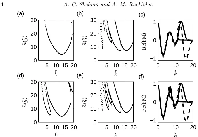
Promotion of patterns with angleθresrequires the quadratic coefficients to be sufficiently large and/or the damping to be sufficiently small. As illustrated in figure 13(a) and (b) for j = {4,5} and in (d) and (e) for j = {4,5,2} although increasing a5 and heading

towards the bicritical point would appear to change the value of the linear damping for the 2˜ω/2 tongue, this is in fact not the dominant effect. This can be seen in figure 13(c) and also in (f) where the Floquet multipliers are plotted for both ˜a5= 0 and a value of

˜

a5 near the bicritical point. It can be seen that increasing the amplitude of the j = 5

mode in the forcing promotes the 5˜ω/2 tongue, as expected, but has little impact on the damping of the other modes. In contrast, now comparing figure 13(c) with (f), we see that the addition of thej= 2 mode does have the effect of reducing the damping of the mode associated with the 2˜ω/2 tongue as seen by an increase in the Floquet Multiplier from approximately 0.5 for ˜a2= 0 to 0.9 for ˜a2= 0.8˜g.

Rather than changing the damping of the weakly damped mode, increasing the am-plitude of the j = 5 mode, so heading towards the bicritical point, has the effect of increasing the quadratic coefficientsα1 andα2: in the limit when ˜a5= 0 the quadratic

coefficients are zero. This is because the temporal resonance condition discussed in sec-tion 4.1 is not met when ˜a5 = 0, so there can be no coupling between the 2˜ω/2 mode

and the 4˜ω/2 mode.

Topaz et al. (2004) consider a weak viscosity limit and show that in the case of j={m, n}forcing the temporal resonance condition results in possible three-wave inter-actions with an (n−m) mode, where one expects

bres=

α|an|2 |λ2|

, (6.1)

where λ2 is the linear damping of the weakly damped mode and α is a coefficient.

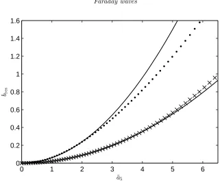
Although this cannot necessarily be expected to apply to the moderate viscosity case of the experiments in Ding & Umbanhowar (2006), we see in figure 14 that the calculated values for bres for the j = {4,5} case have a close to quadratic dependence on a5 as

24 A. C. Skeldon and A. M. Rucklidge

5 10 15 20 0 10 20 30 ˜ a (˜ g ) ˜ k (a)

5 10 15 20 0 10 20 30 ˜ a (˜ g ) ˜ k (b)

5 10 15 20 0 10 20 30 ˜ a (˜ g ) ˜ k (d)

5 10 15 20 0 10 20 30 ˜ a (˜ g ) ˜ k (e)

0 10 20

−1 0 1 (c) R e( F M ) ˜ k

0 10 20

−1 0 1 (f) R e( F M ) ˜ k

Figure 13. Linear stability curves and Floquet multipliers for j = {4,5} and j = {4,5,2}

excitation using parameter values as in Ding & Umbanhowar (2006). (a) and (b) Linear stability curves for ˜f(˜t) = ˜a(cosχcos 4˜ωt˜+ sinχcos 5˜ω˜t), where (a) hasχ= 0 and (b) hasχ= 63◦_{. (c)}

the corresponding Floquet multipliers where the solid line is forχ= 0 and the dashed line is for

χ= 63◦_{. The Floquet multipliers are calculated for ˜afixed at the value for the minimum of the}

4ω/2 tongue. So, forχ= 0,a˜= 4.35˜g, forχ= 63◦_{,˜a= 7.19˜g (d) and (e) Linear stability curves}

for ˜f(˜t) = ˜a(cosχcos 4˜ω˜t+ sinχcos 5˜ω˜t+ ˆa2cos 2˜ω˜t) where (a) hasχ= 0, a2=a˜a2= 0.8gand (b) hasχ= 62◦_,˜a

2 = ˜aˆa2 = 0.8˜g. (c) The corresponding Floquet multipliers where the solid line is for case (d) where ˜a5 = 0 and the dashed line is for (e) where ˜a5 6= 0. The Floquet multipliers are calculated for ˜afixed at the value for the minimum of the 4˜ω/2 tongue. So, for

χ= 0,˜a= 4.40˜g, forχ= 63◦_{,a˜= 7.27˜g.}

that the dominant contribution tobresis given by

bres=α|an|2P2(Φ), (6.2)

where Φ =φp+ 2φm−2φn andP2 is given by

P2=

|λ2|+µa2sin Φ

|λ2|2−µ2a22

,

where µis a coefficient. As a2 →0, equation (6.2) reduces to equation (6.1). However,

fora2non-zero, the effect ofP2is to make the leading order dependence ofbresona2not

purely quadratic, so it is not surprising that for this case, an assumption of quadratic dependence fits less well.

Note that the Φ dependence, which comes from a parameter symmetry, does explain the strong diagonal structure to the figures showing the pattern dependence as a function of two of the phases, see figures 9 and 12.

0 1 2 3 4 5 6 0

0.2 0.4 0.6 0.8 1 1.2 1.4 1.6

˜

a5 bre

s

Figure 14.The value ofbresforj={4,5}(crosses) and forj={4,5,2}(dots) for increasing ˜

a5. The solid lines are proportional to ˜a 2

5. Parameter values as in Ding & Umbanhowar (2006) but with ˜ν= 0.21cm2

s−1 .

where 4˜ω/2,5˜ω/2 and 2˜ω/2 modes all occur simultaneously. The onset boundaries for the three modes for j ={4,5,2} are shown in figure 15: the position of the tri-critical point is at approximately (˜a4,˜a5,˜a2) = (3.5,6.4,1.0)˜g. The situation for j = {6,7,2}

forcing is similar, and one explanation for discrepancies between the weakly nonlinear theory and experimental results may be that they are a consequence of the proximity of the codimension three point. This kind of discrepancy was previously demonstrated by Riyapan (2012) in a comparison of a codimension one and a codimension two analysis of superlattice patterns in a model PDE.

26 A. C. Skeldon and A. M. Rucklidge

0

5

10

0 2 4 6 8 0 0.5 1 1.5

˜ a5(˜g)

˜ a4(˜g)

˜

a2

(˜

g

)

Tricritical point Tricritical point

Figure 15.Surfaces for the onset of modes with frequencies 4˜ω/2,5˜ω/2 and 2˜ω/2. Parameter values as in Ding & Umbanhowar (2006) but with ˜ν= 0.21cm2

s−1 .

the full Navier–Stokes equations even for the moderate viscosity values used in many Faraday experiments.

for our comparison with the work of Epstein & Fineberg (2006) and the opposite sign convention for Ding & Umbanhowar (2006).

Appendix A. Calculating Floquet multipliers

The Floquet multipliers can be calculated by considering the linear stability of the triv-ial solution (2.9) of equation (2.6) and associated boundary conditions to perturbations of the divergence free form

u=

i

k∂zW(z, t),0, W(z, t)

eikx.

This leads to a fourth order equation forW(z, t) for−h/˜ ˜l < z <0

∂t−C −k2+∂zz

−k2

+∂zz

W = 0, (A 1)

with boundary conditions atz=−˜h/˜l,

W(−h/˜ ˜l, t) =∂zW|₋˜_h/˜_l= 0

and atz= 0,

∂tZ =W, k2

+∂zzW = 0,

∂t+C 3k2−∂zz∂zW =− (1 +f(t))k2+Bk4Z.

A finite difference discretization of equation (A 1) and its boundary conditions is then carried out by letting Wn

j =W(zj, tn), j = 0..J, zj =−˜h/˜l+ ˜hj/˜lJ and tn =nδt and Zn_{=Z(tn). The resulting map is of the general form}

A         

Wn+1 1

W2n+1

.. . Wn+1

J−1

Wn+1

J Zn+1

        

=B(tn)

         Wn 1 Wn 2 .. . WJn−1

Wn J Zn         

, (A 2)

whereAandBare (J+ 1)×(J+ 1) matrices given by

A=           

r 1 0

1 r 1 0

0 1 r 1 0

..

. . .. ...

0 1 r 1 0

0 2 r 0

28 A. C. Skeldon and A. M. Rucklidge and B=               

c+Cδt/δz2

b Cδt/δz2

0

b c b Cδt/δz2 ₀

Cδt/δz2 _{b c b Cδt/δz}2 ₀

0 Cδt/δz2 _{b c b Cδt/δz}2 ₀

..

. . .. ...

0 Cδt/δz2 _{b c b Cδt/δz}2 ₀

Cδt/δz2 _{b c−Cδt/δz}2 _{b+d 0}

2Cδt/δz2 _{b+e c+g f}˜n

0 δt 1

               . where

r=− 2 +k2δz2

b= 1−2Ck2

δt−4C δt δz2

c=− 2 +k2

δz2

+C δt

δz2 6 + 4k 2

δz2

+k4

δz4

d=C δt δz2 2−k

2

δz2

e= 1−4Ck2

δt

fn= 2δtδz (1 +f(tn))k2

+Bk4

g=−C δt δz2 2−k

2

δz22

.

The matrixBcontains time dependence through the termfn_(t n).

The map (A 2) is iterated through one period, T, of the drive resulting in a map

WN =DW0 that takesW0 _toWN _{whereN =T /δt. The eigenvalues of the matrixD} then give the required Floquet multipliers.

This paper builds on discussions about pattern formation in the Faraday problem with many individuals over the years. In particular the authors would like to acknowledge the input of Mary Silber, Jeff Porter and Jay Fineberg. We thank the referees for their thorough reading of the paper and their helpful comments.

REFERENCES

Alnahdi, A.S., Niesen, J. & Rucklidge, A.M.2014 Localized patterns in periodically forced systems.SIAM Journal on Applied Dynamical Systems13_{, 1311–1327.}

Arbell, H. & Fineberg, J.1998 Spatial and temporal dynamics of two interacting modes in parametrically driven surface waves.Physical Review Letters81_{, 4384–4387.}

Arbell, H. & Fineberg, J.2000 Temporally harmonic oscillons in Newtonian fluids.Physical Review Letters 85_{, 756–759.}

Arbell, H. & Fineberg, J.2002 Pattern formation in two-frequency forced parametric waves. Physical Review E 65_{, 036224.}

Benjamin, T. B. & Ursell, F.1954 The stability of a plane free surface of a liquid in vertical periodic motion.Proceedings of the Royal Society, London A225_{, 505–515.}

Bodenschatz, E., Pesch, W. & Ahlers, G.2000 Recent developments in Rayleigh–B´enard convection.Annual Reviews of Fluid Mechanics32_{, 709–778.}

Chen, P. & Vi˜nals, J. 1999 Amplitude equation and pattern selection in Faraday waves. Physical Review E 60_{, 559–570.}

Christiansen, B., Alstr¨om, P. & Levinsen, M. T. 1992 Ordered capillary-wave states: Quasicrystals, hexagons, and radial waves.Physical Review Letters 68_{, 2157–2160.} Ding, Y.2006 Pattern formation in multi-frequency driven fluid surface waves. Ph.d. thesis,

Northwestern University.

Ding, Y. & Umbanhowar, P.2006 Enhanced Faraday pattern stability with three-frequency drive.Physical Review E 73_{, 046305.}

Dionne, B., Silber, M. & Skeldon, A. C.1997 Stability results for steady, spatially periodic planforms.Nonlinearity10_{, 321–353.}

Edwards, W. S. & Fauve, S. 1994 Patterns and quasi-patterns in the Faraday experiment. Journal of Fluid Mechanics278_{, 123–148.}

Epstein, T. & Fineberg, J.2004 Control of spatiotemporal disorder in parameterically excited surface waves.Physical Review Letters 92_{, 244502.}

Epstein, T. & Fineberg, J.2006 Grid states and nonlinear selection in parametrically excited surface waves.Physical Review E 73_{, 055302.}

Faraday, M.1831 On the forms and states of fluids on vibrating elastic surfaces.Philosophical Transactions of the Royal Society London121_{, 319–340.}

Iooss, G. & Rucklidge, A.M.2010 On the existence of quasipattern solutions for the Swift– Hohenberg equation.Journal of Nonlinear Science20_{, 361–394.}

Kahouadji, L., P´erinet, N., Tuckerman, L. S., Shin, S., Chergui, J. & Juric, D.2015 Numerical simulation of super-square patterns in faraday waves.arxivp. 1501.04122. Kudrolli, A., Pier, B. & Gollub, J. P.1998 Superlattice patterns in surface waves.Physica

D 123_{, 99–111.}

Kumar, K. & Tuckerman, L. S. 1994 Parametric instability of the interface between two fluids.Journal of Fluid Mechanics279_{, 49–68.}

Lifshitz, R. & Petrich, D. M. 1997 Theoretical model for Faraday waves with multiple-frequency forcing.Physical Review Letters 79_{, 1261–1264.}

Malkus, M. V. R. & Veronis, G.1958 Finite amplitude cellular convection.Journal of Fluid Mechanics 4_{, 225–260.}

Melbourne, I.1999 Steady-state bifurcation with Euclidean symmetry. Transactions of the American Mathematical Society 351_{, 1575–1603.}

M¨uller, H. W. 1994 Model equations for two-dimensional quasipatterns. Physical Review E 49_{, 1273–1277.}

P´erinet, N., Juric, D. & Tuckerman, L. 2009 Numerical simulation of Faraday waves. Journal of Fluid Mechanics635_{, 1–26.}

P´erinet, N., Juric, D. & Tuckerman, L.2012 Alternating hexagonal and striped patterns in Faraday surface waves.Physical Review Letters 109_{, 164501.}

Porter, J. & Silber, M. 2002 Broken symmetries and pattern formation in two-frequency forced Faraday waves.Physical Review Letters 89_{, 054501.}

Porter, J., Topaz, C. M. & Silber, M.2004 Pattern control via multifrequency parametric forcing.Physical Review Letters 93_{, 034502.}

Riyapan, P.2012 Mode interactions and superlattice patterns. Ph.d. thesis, University of Leeds. Rogers, J. L., Schatz, M. F., Brausch, O. & Pesch, W. 2000 Superlattice patterns in vertically oscillated Rayleigh–B´enard convection.Physical Review Letters 85_{, 4281–4284.} Rucklidge, A. M. & Rucklidge, W. J.2003 Convergence properties of the 8, 10 and 12 mode

representations of quasipatterns.Physica D 178_{, 62–82.}

Rucklidge, A. M. & Silber, M.2009 Design of parametrically forced patterns and quasipat-terns.SIAM Journal on Applied Dynamical Systems 8_{, 298–347.}

Rucklidge, A. M., Silber, M. & Skeldon, A. C. 2012 Three-wave interactions and spa-tiotemporal chaos.Physical Review Letters 108_{, 074504.}

Segel, L. A. & Stuart, J. T.1962 On the question of the preferred mode in cellular thermal convection.Journal of Fluid Mechanics13_{, 289–306.}