This is a repository copy of Context sensitive cardiac x-ray imaging: a machine vision approach to x-ray dose control.
White Rose Research Online URL for this paper: http://eprints.whiterose.ac.uk/97512/
Version: Accepted Version
Article:
Kengyelics, SM, Gislason-Lee, AJ, Keeble, C orcid.org/0000-0003-1633-8842 et al. (2 more authors) (2015) Context sensitive cardiac x-ray imaging: a machine vision approach to x-ray dose control. Journal of Electronic Imaging, 24 (5). ARTN 051002. ISSN
1017-9909
https://doi.org/10.1117/1.JEI.24.5.051002
Kengyelics, SM, Gislason-Lee, AJ, Keeble, C , Magee, DR and Davies, AG (2015) Context sensitive cardiac x-ray imaging: a machine vision approach to x-ray dose control. Journal of Electronic Imaging, 24 (5). ARTN 051002. http://doi.org/10.1117/1.JEI.24.5.051002 (c) 2015 SPIE and IS&T. One print or electronic copy may be made for personal use only. Systematic electronic or print reproduction and distribution, duplication of any material in this paper for a fee or for commercial purposes, or modification of the content of the paper are prohibited.
[email protected] https://eprints.whiterose.ac.uk/
Reuse
Unless indicated otherwise, fulltext items are protected by copyright with all rights reserved. The copyright exception in section 29 of the Copyright, Designs and Patents Act 1988 allows the making of a single copy solely for the purpose of non-commercial research or private study within the limits of fair dealing. The publisher or other rights-holder may allow further reproduction and re-use of this version - refer to the White Rose Research Online record for this item. Where records identify the publisher as the copyright holder, users can verify any specific terms of use on the publisher’s website.
Takedown
If you consider content in White Rose Research Online to be in breach of UK law, please notify us by
Context sensitive cardiac x-ray imaging: A machine vision approach
to x-ray dose control
Stephen M. Kengyelicsa, Amber Gislason-Leea, Claire Keeblea, Derek Mageeb, and Andrew G. Daviesa
aLeeds Institute of Cardiovascular and Metabolic Medicine, Division of Biomedical Imaging, University of Leeds, Worsley Building, Clarendon Way, Leeds LS2 9JT, United Kingdom
bSchool of Computing, University of Leeds, EC Stoner Building, Leeds, LS2 9JT, United Kingdom
Abstract. Modern cardiac x-ray imaging systems regulate their radiation output based on the thickness of the patient, to maintain an acceptable signal at the input of the x-ray detector. This approach does not account for the context of the examination, or the content of the image displayed. We have developed a machine vision algorithm that detects iodine filled blood vessels and fits an idealized vessel model with key parameters of contrast, diameter and linear attenuation coefficient. The spatio-temporal distribution of the linear attenuation coefficient samples, when arranged appropriately, can be described by a simple linear relationship, despite the complexity of scene information. The algorithm was tested on static anthropomorphic chest phantom images under different radiographic factors and 60 dynamic clinical image sequences. It was found to be robust, and sensitive to changes in vessel contrast resulting from variations in system parameters. The machine vision algorithm has the potential of extracting real-time context sensitive information that may be used to augment existing dose control strategies.
Keywords:cardiac, x-ray, contrast, machine vision.
Address all correspondence to: Stephen M. Kengyelics, Leeds Institute of Cardiovascular and Metabolic Medicine, Division of Biomedical Imaging, University of Leeds, Worsley Building, Clarendon Way, Leeds LS2 9JT, United Kingdom; Tel: +44 (0)113 3438317; E-mail: [email protected]
1 Introduction
In 2012 ischaemic heart disease was the main cause of death worldwide, claiming an estimated
7.4 million lives.1 Percutaneous coronary intervention (PCI) is an effective and minimally invasive
treatment for cardiovascular disease resulting from a narrowing of coronary arteries. It works by
mechanically improving the flow of blood to the heart.2–4 The narrowing of the coronary arteries is
caused by atherosclerosis, a build-up of fatty deposits, referred to as plaques, on the inner surface
of the vessel wall. This may result in the heart muscle becoming starved of oxygen and nutrients,
leading to chest pain or a heart attack, possibly causing permanent damage to the heart which may
PCI procedures may involve several stages. These stages critically depend on the capability
of x-ray and electronic imaging systems to adequately represent anatomical features, such that
the clinical task can be achieved. Clinicians examine moving real-time images of the coronary
arteries using an angiogram, where the blood vessels supplying the heart are made opaque to
x-rays by injecting an iodine-based contrast agent into the vessel lumen. These are subsequently
visualised using an x-ray detector and display. Ordinarily, images are acquired at 15 frames per
second, resulting in sequences of anywhere between approximately 30–100 frames, though there
is considerable variation.
The critical dependence on x-ray imaging during PCI procedures requires the use of ionizing
radiation and its concomitant hazard to both patients and staff.5, 6 Lowering radiation dose is
ad-vantageous, but any reduction may result in the deterioration of the diagnostic visual information
that may compromise patient care.7 The principle regulating x-ray dose to patients is to reduce
it to a level that is as low as reasonably achievable. This so-called ALARA principle, ensures
that the radiation dose is sufficient to achieve the clinical task. In practice, this level is difficult
to establish on an individual basis, as requirements differ by patient and task, and depend on the
system geometry and settings employed.
The purpose of this paper is to propose a method to provide some contextual information that
may be used to augment existing dose control strategies.
The contrast of iodine filled blood vessels defines how well the vessel structures stand out
from surrounding anatomy. This is a key component for producing high-quality, diagnostically
acceptable, cardiac images. Notionally, the higher the level of contrast the better the vessels are
visualized, leading to greater diagnostic utility that might be referred to as image quality in this
de-scribed is complex and is not discussed here. It is sufficient to note, however, that currently cardiac
imaging systems do not monitor or attempt to predict the level of image contrast in PCI procedures,
despite being a key facet in producing clinically acceptable images.
A machine vision approach is investigated to detect iodine filled blood vessels, extract sample
profiles orthogonal to their centre lines, and fit an idealized vessel model. Populations of contrast,
vessel diameter, and linear attenuation coefficients are extracted. We show that the spatio-temporal
distribution of the linear attenuation coefficient population, when arranged appropriately, can be
described by a simple linear relationship, despite the complexity of scene information. This
rela-tionship has the potential to provide real-time context based image information, that may be used
to augment the existing ADRC strategy to deliver adequate image quality at the lowest radiation
dose. Thus, the ALARA principle can be implemented on an individual basis.
2 Methodology
2.1 Modification of automatic dose rate control
Currently, most modern cardiac x-ray imaging systems regulate their radiation output by adjusting
several system parameters to maintain a constant average output signal from the x-ray detector.
The control system for the cardiac x-ray imaging unit, specific to this study, is illustrated in
Fig-ure (1). The patient is positioned on a table, face-up, between the x-ray source and the detector.
The source and detector are mounted on a gantry to keep the detector orthogonal to the central
axis of the x-ray beam, and may be rotated around the patient from left to right, and from head to
toes, to produce different projections. The table height and source-to-detector distance may also
be adjusted independently of the gantry projection angles. These degrees of freedom allow the
Requested Output Signal Anti-scatter Grid X-ray Flat Detector Patient Table X-ray Tube System Mode Selection
Compute kVp, mA, ms
Generator Average Detector Output Signal Difference Signal Beam Filtration Update Factors Real-time Image Information Beam Shutters
Fig 1Cardiac x-ray imaging system: Feedback control diagram.
obtain multiple views of the same feature from different angles. Referring to Figure (1), if the
average output of the x-ray detector decreases with respect to that requested by the system mode
selection, a difference signal is generated and used to calculate a new set of system parameters
that will increase the output of the x-ray source to reduce the difference signal to zero. The
sys-tem parameters calculated are the x-ray tube voltage (kVp), current (mA), and pulse width (ms).
The average output of the detector is calculated per image frame using the digital values contained
within a predefined circular measuring field. Overall the system is designed to maintain a constant
average detector signal, irrespective of variations in patient anatomy and system geometry, up to
the point where statutory stipulations limit any further increase in the x-ray radiation output.
While this form of automatic dose rate control (ADRC) scheme is effective, it does not provide
any information derived from the available image data. We propose to modify the feedback control
scheme shown Figure (1) by using real-time image information to augment the existing feedback
X-ray photons input
Detected Profile
b Vessel Cross-Section
Background Anatomy
s
Fig 2Detected profile of blood vessel filled with contrast agent.
2.2 Image information extraction
The contrast of iodine-filled vessels is defined here according to Equation (1), wheresis the peak digital value of the profile of the vessel cross-section andbis the average digital value of the profile outside the extent of the vessel. Referring to Figure (2), x-ray photons penetrating the patient form
a digital image of the vessel and the background anatomy. Contrast is measured according to our
definition from a profileP(x)extracted from the image that is orthogonal to the center-line of the vessel, wherexis displacement in pixel units. The profile is defined to overlap either edge of the vessel by one-half of the vessel diameter. The definition assumes a linear relationship between the
recorded digital value and incident x-ray photon fluence.
C= s−b
b (1)
There are a number of challenges in obtaining useful measurements of iodine-filled coronary
[image:6.612.214.407.75.294.2]acquisi-tion, the scene is continuously changing due to the inflow and outflow of contrast agent, cardiac
motion, respiratory and minor patient movement. In some instances there is movement of the
en-tire patient, as the clinician repositions them to optimise the view. Due to this dynamic nature and
with the presence of multiple, often overlaying, vessel structures, it in not currently possible to
de-tect and segment complete coronary artery networks reliably. In addition, coronary artery trees are
composed of vessels with a range of different diameters, and thus single measurements would be
of limited value, since larger vessels will produce higher contrast just by virtue of containing more
x-ray attenuating material. For such measurements to be useful it would also be necessary to relate
them to the vessel width and track the exact point where the measurement was made from frame to
frame. It is possible to detect, segment and measure the diameter of sections of vessel in individual
image frames, but it is difficult to define a particular location on a vessel that might be re-identified
on a subsequent image frame. This is due to the dynamic nature of the scene described above.
Our approach avoids these problems by not attempting to fully segment the coronary artery
tree, or identify individual features from frame to frame. Instead, partial segmentation and
mor-phological operations are used to identify multiple points representing the center-lines of vessels
segments, for a range of vessel diameters. These are remote from bifurcations, and not overlaying
any complex anatomical structures. Using these points, cross-sectional profiles are extracted that
are orthogonal to the length of the vessel. A simple model of a tubular blood vessel filled with a
contrast agent is fitted to each profile. The key parameters of the model are the vessel diameter,
contrast, and linear attenuation coefficient.
These parameters may be viewed as referred values, in that it is assumed they would result
from measuring an idealized circular vessel. This idealized vessel has its long axis imaged in
a mono-energetic x-ray source, regardless of its displacement in the image field. In practice, this
assumption is not true for a number of reasons. For example, a blood vessel may be orientated such
that it is foreshortened with respect to the detector, resulting in a higher contrast value. However,
the foreshortened vessel would appear darker to an observer compared to the same vessel that was
not foreshortened. So despite not having an accurate contrast value for the vessel, if it were imaged
ideally, the referred contrast offers practical values that are related to contrast presented to the user.
The parameters, for all cross-sectional profiles, form a population of values both spatially,
across the extent of a single frame, and temporally from frame to frame. The referred contrast
and diameter parameters are useful metrics relating to observer perception. The linear attenuation
coefficients are more useful in reflecting changes in the concentration of the contrast agent or
variations in the system settings, such as the x-ray beam energy or the amount of scattered x-ray
photons incident on the detector.
In addition, the population of linear attenuation estimates, when appropriately arranged, was
found to have a linear relationship over the majority of values contained in an image frame. This
relationship provides a simple categorisation of the linear attenuation coefficients for a single image
frame as a whole. It is also found to be relatively stable from frame to frame, and as such has the
potential to provide context sensitive feedback to augment the ADRC, despite the complexity of
the scene.
2.3 Data acquisition
Digital image sequences were obtained from a modern cardiac x-ray imaging system, used
rou-tinely for PCI procedures in the Leeds General Infirmary, United Kingdom (Allura FD10, Philips
The sequences were acquired prior to the application of any non-linear image processing
al-gorithms, via a propriety data capture device installed by the manufacturer. The only processing
applied prior to capture, was linear scaling and a dynamic range compression look-up table. Both
test phantom and clinical images were acquired. Each image sequence contained approximately
30-50 image frames of1024×1024pixels.
Test images were acquired using an anthropomorphic chest phantom (Radiology Support
De-vices, Alderson Phantoms, Long Beach, USA) containing a left coronary artery (LCA) filled with
contrast agent. The phantom was arranged on the examination table in a posteroanterior
projec-tion, and the heart positioned at the isocenter; the center of rotation of the x-ray tube and detector.
This was prior to angulation of the gantry, to optimize the view of the coronary arteries. An air
gap of 10 cm was set between the exit surface of the phantom and the entrance to the detector,
reflecting clinical practice. The 15 cm field size was selected and a series of images of the LCA
was acquired at peak x-ray tube voltages of: 50, 70, 90, and 110 kVp, using the digital-acquisition
mode. Approximately 50 image frames per sequence were acquired. Adjustment of the kVp, mA,
and ms, was performed manually by over-riding the ADRC. This series provided static images
with the same geometrical arrangement of the LCA, but with decreasing contrast values due to the
increase in kVp.
Clinical images came from different patient examinations, and comprised 30 left coronary
artery (LCA) and 30 right coronary (RCA) sequences, acquired at 15 frames per second, using
the digital-acquisition mode and 15 cm field size. The image sequences chosen did not contain
any additional catheters, guide wires or other surgical devices other than the main catheter used to
2.4 Measurement algorithm description
A machine vision algorithm was developed in MATLAB8and can be divided into two broad
oper-ations: (1) candidate vessel location and (2) vessel parameter estimation.
2.4.1 Candidate vessel location
This section of the algorithm returned coordinates of candidate points within a single image frame
which are on the center-lines of iodine-filed coronary arteries, and within a specified range of
di-ameters and lengths in the image plane. The algorithm is applied to all image frames in a sequence.
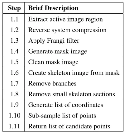
[image:10.612.205.404.342.557.2]The major steps of this section of the algorithm are shown in Table (1).
Table 1Candidate vessel location: List of algorithm steps.
Step Brief Description
1.1 Extract active image region
1.2 Reverse system compression
1.3 Apply Frangi filter
1.4 Generate mask image
1.5 Clean mask image
1.6 Create skeleton image from mask
1.7 Remove branches
1.8 Remove small skeleton sections
1.9 Generate list of coordinates
1.10 Sub-sample list of points
1.11 Return list of candidate points
(1.1) Extract active image region: The raw data sequences contained dark regions at their
periphery produced by the x-ray shuttering, that is used to restrict the irradiation of the patient to
only those areas of clinical interest. For the image sequences in this study, the edges of the shutters
produce penumbral effects in the image plane, at the interface of the clinical image information.
misidentified as vessel structures, so prior to further analysis the clinical image data is extracted
from inside the region defined by the shutters.
The vertical shutters were identified by averaging the pixel values in the vertical direction
to form a profile that has a length equal to the width of the image. The profile is smoothed,
differentiated, and a threshold applied, to identify the edges of the shutters which generally produce
the two largest gradients in the image. Occasionally other structures contained in the active image
area can produce high gradients, such as surgical instruments or devices. However, the shutters
can be identified as they work as a pair, closing from the periphery of an image to the centre, so
spurious edges may easily be identified. Identification of the horizontal shutters was performed
in the same way but in the orthogonal direction. Having identified vertical and horizontal shutter
positions, the active image area was extracted from the image frame.
(1.2) Reverse system compression: The digital values were transformed using a look-up table
to invert the dynamic range compression applied by the imaging system prior to data capture. This
restored a linear relationship between increments of the input x-ray exposure and digital values.
(1.3) Apply Frangi filter: A Frangi filter9 was applied to the image sequence at five different
scales to cover the vessel sizes of interest. The filter identifies tube-like structures within an image
at specified scales. The algorithm returns a number of responses, including a direction image that
contains the orientation of the eigenvectors for all scales.
(1.4) Generate mask image: A binary mask image of the detected vessel locations was
gener-ated by applying a threshold to a standard deviation map of the direction image, for local regions
of interest of 3×3 pixels. Generally, the eigenvectors in the local vicinity of a vessel will all
have similar values. Therefore, they will have a low standard deviation in comparison with other
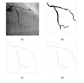
(a) (b)
(c) (d)
Fig 3 Candidate vessel location (a) LCA single frame (b) Binary Mask (c) Skeleton (d) Skeleton with bifurcations removed.
image, was chosen to generate the mask. This is because it is also required later for calculating
the direction of profiles orthogonal to the vessel center-lines, and is thus more computationally
efficient.
(1.5) Clean mask image: Noise was removed using standard morphological operations. An
example of a binary mask derived using steps 1.1 to 1.5 for a single frame of an LCA sequence,
Figure (3a), is shown in Figure (3b).
(1.6) Create skeleton image from mask: A skeleton was produced by thinning the mask image
as shown in Figure (3c).
(1.7) Remove branches: Bifurcations in the mask and regions around them are removed, as
only measurements across single unobstructed sections of vessel were of interest, see Figure (3d).
[image:12.612.166.448.76.355.2]and lengths below 30 pixel units were not included in the analysis.
(1.9) Generate list of coordinates: Any non-zero points in the resulting skeleton image represent
candidates for the center-lines of vessel segments. An ordered set of coordinates of non-zero points
were generated per vessel, such that the first and last points for each vessel corresponded to the start
and finish of the vessel. Intermediate points were sorted sequentially according to their position
along its length between the start and the finish points.
(1.10) Sub-sample list of points: The user may sub-sample the list of candidates by
retain-ing everynth point, as not all points are required to obtain a good representation of the contrast
distribution along a vessel.
(1.11) Return list of candidate points: Return the coordinates of candidate points for each vessel
within each frame.
2.4.2 Vessel parameter estimation
This part of the algorithm returned estimates of the vessel parameters: contrast, vessel diameter,
and linear attenuation coefficient. The estimates were associated with each valid candidate point
returned using the algorithm in section 2.4.1, by fitting an idealized vessel profile model orthogonal
to the center-line.
The major steps of this section of the algorithm are shown in Table (2).
(2.1) Determine the vessel direction: The orientation of the long axis of the vessel at the
loca-tion of the candidate point, is determined from the Frangi direcloca-tion image.
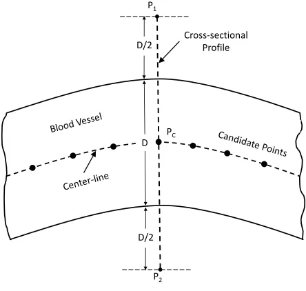
The overall aim of steps (2.2) to (2.7) is to extract a profileP between two points[P1, P2]. The line between the points is orthogonal to the center-line of the vessel and overlaps it by one half of
Table 2Vessel parameter estimation: List of algorithm steps.
Step Brief Description
2.1 Determine the vessel direction
2.2 Estimate location of two points orthogonal to vessel direction on either side
2.3 Skip pairs of points if either is outside image
2.4 Use points to estimate vessel diameterDfrom mask image
2.5 Re-estimate location of points orthogonal to vessel using (1) and (4)
2.6 Extract profile,Pbetween pairs of points from (5)
2.7 CalculateV1andV2- the location of the upper/lower limits of the vessel inP
2.8 Fit linear curve toPusing points outside the region of the vessel
2.9 Skip profiles exceeding defined gradient limit
2.10 Subtract the curve fit fromP
2.11 Normalise the result to unity yieldingPN
2.12 Fit the vessel model toPN using start valuesPcandD
2.13 Skip profiles that produces agoodness-of-fitoutside defined limit
2.14 Return contrast, vessel diameter, and linear attenuation coefficient estimates
D/2 P1
P2
D PC
D/2
Cross-sectional Profile
Fig 4Cross-sectional profile location.
as illustrated in Figure (4). The overlap provides a consistent approach to considering the contrast
[image:14.612.196.418.390.601.2](2.2) Estimate location of two points orthogonal to vessel direction on either side: Initially the
diameter of the vessel is not known, so a guess is made for two points. These points are equally
spaced either side of the candidate point, at a distance of 20 pixel units, and orthogonal to the
direction determined in (2.1). The placement of these points allows for the largest vessel size
accommodated by the scales initially set for the Frangi filter.
(2.3) Skip pairs of points if either is outside image: Inevitably, some candidate points close
to the edge of an image will generate points from (2.2) that are outside the image and, therefore,
excluded from the analysis.
(2.4) Use points to estimate vessel diameter D from mask image: A binary image is created that represents the two points generated from (2.2) and all the points in a straight line between
them. This image is logical multiplied with the mask generated in steps (1.1) to (1.5). The distance
between the endpoints of the resulting profile represents an estimate of the vessel diameter D, orthogonal to the candidate center-line point.
(2.5) Re-estimate locations of the two points orthogonal to the vessel, using the vessel direction
image from (2.1), and the estimate of the vessel diameter from (2.4).
(2.6) Extract profile, P between the pair of points, assigned to be [P1, P2], generated in step (2.5).
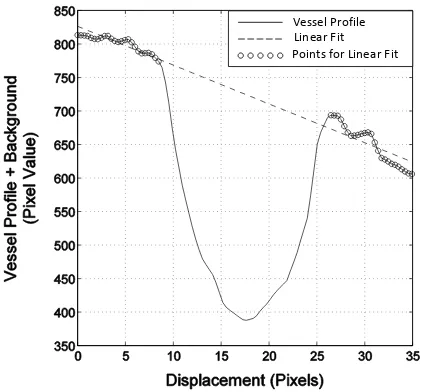
The purpose of steps (2.7) to (2.10) is to remove trends from P associated with background anatomy, as illustrated in Figure (5), to provide an average single background level for the contrast
estimation. A linear curve fit is applied to the regions of the vessel profile either side of the vessel,
and then subtracted from the profile. The result is then inverted and normalized to a form suitable
Vessel Profile Linear Fit Points for Linear Fit
Fig 5Example of background trend removal from the vessel profile.
(2.7) Calculate V1 and V2 - the location of the limits of the vessel in P: These values are calculated from the vessel width estimate and the candidate center-line point position: V1 =Pc−
D/2andV2 =Pc+D/2.
(2.8) Fit linear curve toP using points outside the region of the vessel: The regions of support for the linear curve fit are in the rangesP1 toV1, andV2 toP2.
(2.9) Skip profiles exceeding defined gradient limit: Extreme gradients (> 30) indicate the presence of either another vessel, or possibly part of a medical device in the vicinity, and are
excluded from the analysis.
(2.10) Subtract the curve fit fromP.
(2.11) Normalise the result to unity yielding PN: Normalize the result according to
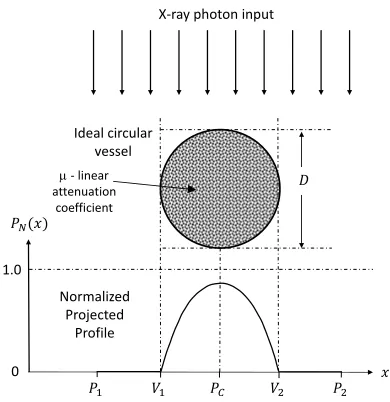
[image:16.612.200.411.88.284.2]Ideal circular vessel
X-ray photon input
Normalized Projected
Profile
0 1.0
m - linear attenuation
coefficient
Fig 6Normalized cross-sectional profile.
PN(x) = 1− P(x) Pmax
(2)
(2.12)–(2.14) fit an idealized vessel profile model to PN and return the parameters: contrast,
vessel diameter, and linear attenuation coefficient. The vessel model is derived by calculating the
cross-sectional profile of the attenuation of an ideal circular blood vessel. This ideal vessel is filled
with a contrast agent with a linear attenuation coefficientµ, and imaged using a mono-energetic, parallel beam x-ray source, together with an ideal detector, as illustrated in Figure (6).
The vessel model is given by Equation (3), whereµn =µ/Dis the linear attenuation coefficient
normalized to the vessel diameter.
PM(x) =
1−e−µnD|cos π
D(x−Pc)
| x∈[V1, V2]
0 elsewhere.
(3)
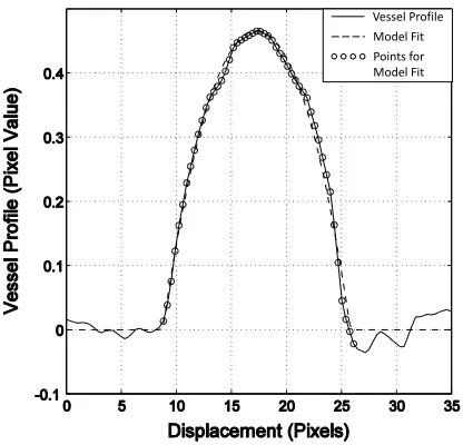
[image:17.612.204.399.81.282.2]Vessel Profile
Model Fit Points for Model Fit
Fig 7Example of ideal vessel model fit to measured cross-sectional profile.
independently for the fitting algorithm to converge more easily, then µ is returned once fitting is complete. Contrast is the maximum value of PM(x). Note thatµ is expressed per pixel unit.
Conventionally, the linear attenuation coefficient is a material specific constant that describes the
fraction of a narrow beam of mono-energetic x-rays that is absorbed, or scattered, per unit
thick-ness. Image contrast arises due to differences in the thickness and linear attenuation coefficients
of a material, and the structures surrounding it. Here we model the measured contrast profile
aris-ing from an ideal circular vessel, filled with some material of linear attenuation coefficientµ, that accounts for the measured diameter and contrast of the vessel, with respect to its local background.
(2.12) Fit the vessel model to PN using start values Pc and D: A non-linear least-squares
Levenberg-Marquardt algorithm is used to fit PN, in the region of support between the points V1 and V2. An example of the model fit of the profile of a iodine-filled blood vessel is shown in Figure (7). The start values, together with the use of µn, greatly reduce the number of iterations
[image:18.612.206.414.83.283.2](2.13) Skip profiles that produces a goodness-of-fit outside the defined limit: Profiles resulting
in a mean square error of greater than1×10−3, calculated within the region of support, when fitted
to the model, are excluded from further analysis. The mean squared error is a scalar estimate of
the variance of the error term of the model.
(2.14) Return the contrast, vessel diameter and linear attenuation estimates.
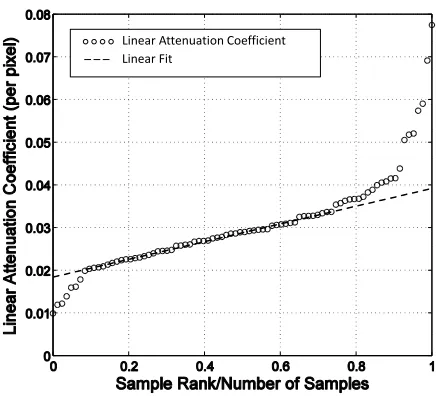
2.5 Data normalization
The population of samples for the linear attenuation coefficients for each image frame are sorted
from lowest to highest value. They are then arranged against an axis of sample rank normalized to
the number of samples, as illustrated in Figure (8), for a single frame from an LCA sequence. This
normalization of the abscissa allows the intercomparison of the values on a common scale from
frame to frame, and sequence to sequence. Note that over the region[0.1,0.75]the relationship is approximately linear for this sequence. This was found to be true for all LCA and RCA images
contained in the 60 clinical test sequences for a region[0.25,0.75].
2.6 Algorithm testing
The purpose of developing the automatic measurement algorithm was to estimate the parameters
(contrast, diameter, and linear attenuation) of iodine filled vessels, over a significantly
represen-tative extent of the coronary artery tree. As such, the algorithm need not identify all the vessels
present. It should, however, measure the contrast values with a precision comparable with a
man-ual measurement technique. Hence, two test criteria were defined. Firstly, if present the algorithm
must automatically locate a minimum of 75% of the length of one section of iodine filled coronary
Linear Attenuation Coefficient Linear Fit
Fig 8Linear attenuation coefficients: Data normalization.
5% compared to an appropriate manual measurement technique.
The first criteria was tested by running the algorithm on the 60 clinical test image sequences.
Each sequence was then displayed to a user a single frame at a time. The positions of iodine
filled coronary arteries identified by the algorithm were overlaid as coloured contour lines on the
display, along with a numeric graticule. The user recorded the approximate total length of the
longest vessel, either fully or partially identified by the algorithm, and the length of the identified
portion of that vessel.
For the second criteria, the algorithm was used to measure the contrast level of single sections of
iodine vessel. The regions of interest were100×100pixels, from a single image frame, extracted
from each of 60 test sequences. For each image the algorithm automatically located the vessel,
estimated the center-line, performed the model curve fit, and calculated the contrast at all the
sample points along its length. The contrast results (around 30–50 in each region) were then
[image:20.612.196.414.80.278.2]For each of the regions of interest, the vessel contrast was measured using a manual technique.
Ten sample locations along the vessel center-line were used and the results averaged. The manual
technique used a software-based measurement tool, that allows a user to position lines and markers
on the image frames displayed on-screen. Profiles could also be generated and measured against
numeric scales. For each image the user marked the edge of the vessel boundary by inspection,
and then defined a center-line equidistant from each boundary. Ten equally spaced sample points
were marked along the center-line, within the bounded region of interest, and orthogonal profiles
generated at these locations. The profile values were transformed according to Equation (2) and
displayed as a graph of contrast against displacement. The user estimated the peak contrast level
from an overlaid numerically labelled graticule.
The sensitivity of the algorithm to variations in the attenuation coefficient of the contrast agent
was tested. Testing consisted of applying it to the series of chest phantom image acquired at a
range of kVp values, as described in section 2.3.
The temporal behaviour of the algorithm to variations in the cardiac image scene, from frame
to frame was also tested. The referred linear attenuation coefficient at the normalized abscissa
value of 0.5, known as the mid-value, see Figure (8), was assessed as a function of frame number,
for three clinical image sequences.
3 Results
For the first test criteria, the algorithm successfully located a minimum of 75% of the length of
one section of iodine filled coronary artery if present. This was true for every image frame of a
sequence, for the 60 test image sequences examined.
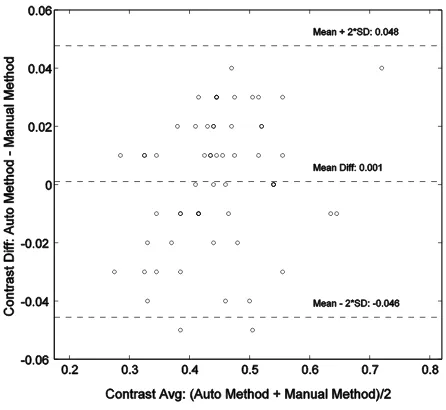
Fig 9Bland-Altman plot comparing the machine vision algorithm with a manual measurement technique.
0.05. This indicated good reproducibility for both measurement methods, and also supported the
assumption that the profile of the vessel did not change significantly, over the small pre-defined
regions of interest.
Recall the population of samples for the linear attenuation coefficients, as illustrated in
Fig-ure (8), is approximately linear in the region[0.1,0.75]of the x-axis, for all 60 image sequences. This relationship provides a simple categorisation of the linear attenuation coefficients for a single
image frame as a whole, despite the complexity of the scene. The departure from a linear
rela-tionship below this range, is thought to be due to the partial filling of some the blood vessels with
contrast agent. Above this range it is thought to be due to foreshortening of some of vessels as they
wrap around the heart.
Figure (9) shows a Bland-Altman plot comparing the automatic and manual measurement
methods, indicating a mean bias of 0.001. The 95% confidence limits: -0.046 to 0.048 are
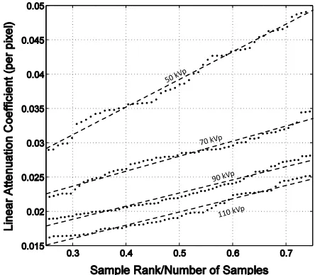
[image:22.612.193.416.84.289.2]Fig 10Attenuation coefficients for an anthropomorphic chest phantom.
Figure (10) shows the linear attenuation coefficients for anthropomorphic chest phantom
im-ages. It demonstrates that the measurement algorithm is sensitive to variations in linear attenuation
coefficient, resulting from changes in the x-ray system settings.
Figure (11) shows the referred mid-value linear attenuation coefficients as a function of frame
number, for three LCA clinical image sequences. The sequences were chosen as they shared
similar system geometry and displayed anatomy, and only differed significantly in the kVp value.
These results show that the mid-value linear attenuation coefficient is stable over time. This is
despite the variation of scene information, resulting from the transit of contrast agent and complex
movement of the heart. The larger deviation observed for 72 kVp values is due to some of the
vessels moving over background anatomical features, from one image frame to the next, which
[image:23.612.192.414.86.280.2]72 kVp
79 kVp
91 kVp
Fig 11Attenuation coefficients for clinical image sequences as a function of frame number.
4 Discussion and conclusions
We have developed an automatic machine vision algorithm to parametrize the contrast in iodine
filled coronary arteries. The overall aim was to provide context sensitive imaging information, for
use in the dose control feedback system of a modern cardiac imaging system.
Contrast is not the only important aspect of image quality for cardiac imaging. Image noise,
spatio-temporal resolution properties, and the application of specialist image processing, are also
critically important. We selected contrast for our initial investigation, as the x-ray imaging system
has several convenient degrees of freedom by which to influence it. These include the x-ray tube
voltage (kVp), x-ray beam filtration, the source-to-detector distance (which influences scatter and
therefore contrast), and the anti-scatter grid.
The algorithm was required to identify a representative sample of vessels across the coronary
artery tree in each image frame. It was also need to make estimates of contrast, diameter and linear
[image:24.612.194.415.93.288.2]results presented have demonstrated that both requirements have been met for the 60 clinical image
sequences tested. The algorithm is computationally inexpensive and has the potential of working
in real-time. In addition, it has been demonstrated that the algorithm is sensitive to changes in
system settings, that directly affect the linear attenuation coefficient of the contrast agent. It also
provides a robust measurement over time, even in the presence of variable scene information.
Future work will incorporate the referred linear attenuation information into the dose control
feedback loop for a modern cardiac x-ray imaging system. In addition, the contrast results will be
compared to observer experience of images, concerning the perceived contrast and acceptability of
images, to achieve a clinical objective.
Acknowledgments
This work has been performed in the project PANORAMA, funded by grants from Belgium, Italy,
France, the Netherlands, and the United Kingdom, and the ENIAC Joint Undertaking.
References
1 World Health Organisation, “The top 10 causes of death, Factsheet no 310.”http://www.
who.int/mediacentre/factsheets/fs310/en/# (2014). Accessed 17th June
2014.
2 P. Ludman, National Audit of Percutaneous Coronary Interventional Procedures Public
Re-port, British Cardiovascular Intervention Society (2011).
3 E. Grech, “Percutaneous coronary intervention. I. History and development,”Brit. Med. J.326,
1080–1082 (2003).
4 E. Grech, “Percutaneous coronary intervention. II. The procedure,” Brit. Med. J.326, 1137–
5 M. J. Eisenberg, J. Afilalo, P. R. Lawler, M. Abrahamowicz, H. Richard, and L. Pilote,
“Can-cer risk related to low-dose ionizing radiation from cardiac imaging in patients after acute
myocardial infarction,”CMAJ183(4), 430–436 (2011).
6 D. ˘Zontar, D. Kuhelj, D. ˘Skrk, and U. Zde˘sar, “Patient peak skin doses from cardiac
interven-tional procedures,”Radiat. Prot. Dosim.139, 162–165 (2010).
7 A. J. Gislason-Lee, A. R. Cowen, and A. G. Davies, “Dose optimization in cardiac x-ray
imaging,”Med. Phys.40, 091911–1–11 (2013).
8 MATLAB,Version 8.3.0.532 (R2014a), The MathWorks Inc., Natick, Massachusetts (2014).
9 A. Frangi, W. Niessen, K. Vincken, and M. Viergever, “Multiscale vessel enhancement
fil-tering,” in Medical Image Computing and Computer-Assisted Interventation MICCAI98,
W. Wells, A. Colchester, and S. Delp, Eds.,Lecture Notes in Computer Science1496, 130–137,
Springer Berlin Heidelberg (1998).
Stephen M. Kengyelicsreceived his MSc degree in physics in 1997 from the University of Leeds
United Kingdom. He received a BEng degree in electrical and electronic engineering from the
University of Plymouth in 1991.
Biographies and photographs of the other authors are not available.
List of Figures
1 Cardiac x-ray imaging system: Feedback control diagram. . . 4
2 Detected profile of blood vessel filled with contrast agent. . . 5
3 Candidate vessel location . . . 11
5 Example of background trend removal from vessel profile. . . 15
6 Normalized cross-sectional profile. . . 16
7 Example of ideal vessel model fit to measured cross-sectional profile. . . 17
8 Linear attenuation coefficients: Data normalization. . . 19
9 Bland-Altman plot comparing the machine vision algorithm with a manual mea-surement technique. . . 21
10 Attenuation coefficients for an anthropomorphic chest phantom. . . 22