Fitting adjusted limited dependent variable mixture models to EQ-5D

(1)

Editors

H. Joseph Newton

Department of Statistics Texas A&M University College Station, Texas [email protected]

Nicholas J. Cox

Department of Geography Durham University Durham, UK

[email protected]

Associate Editors

Christopher F. Baum, Boston College

Nathaniel Beck, New York University

Rino Bellocco, Karolinska Institutet, Sweden, and University of Milano-Bicocca, Italy

Maarten L. Buis, University of Konstanz, Germany

A. Colin Cameron, University of California–Davis

Mario A. Cleves, University of Arkansas for Medical Sciences

William D. Dupont, Vanderbilt University

Philip Ender, University of California–Los Angeles

David Epstein, Columbia University

Allan Gregory, Queen’s University

James Hardin, University of South Carolina

Ben Jann, University of Bern, Switzerland

Stephen Jenkins, London School of Economics and Political Science

Ulrich Kohler, University of Potsdam, Germany

Frauke Kreuter, Univ. of Maryland–College Park

Peter A. Lachenbruch, Oregon State University

Jens Lauritsen, Odense University Hospital

Stanley Lemeshow, Ohio State University

J. Scott Long, Indiana University

Roger Newson, Imperial College, London

Austin Nichols, Urban Institute, Washington DC

Marcello Pagano, Harvard School of Public Health

Sophia Rabe-Hesketh, Univ. of California–Berkeley

J. Patrick Royston, MRC Clinical Trials Unit, London

Philip Ryan, University of Adelaide

Mark E. Schaffer, Heriot-Watt Univ., Edinburgh

Jeroen Weesie, Utrecht University

Ian White, MRC Biostatistics Unit, Cambridge

Nicholas J. G. Winter, University of Virginia

Jeffrey Wooldridge, Michigan State University

Stata Press Editorial Manager Lisa Gilmore

Stata Press Copy Editors

David Culwell,Shelbi Seiner, andDeirdre Skaggs

TheStata Journalpublishes reviewed papers together with shorter notes or comments, regular columns, book reviews, and other material of interest to Stata users. Examples of the types of papers include 1) expository papers that link the use of Stata commands or programs to associated principles, such as those that will serve as tutorials for users first encountering a new field of statistics or a major new technique; 2) papers that go “beyond the Stata manual” in explaining key features or uses of Stata that are of interest to intermediate or advanced users of Stata; 3) papers that discuss new commands or Stata programs of interest either to a wide spectrum of users (e.g., in data management or graphics) or to some large segment of Stata users (e.g., in survey statistics, survival analysis, panel analysis, or limited dependent variable modeling); 4) papers analyzing the statistical properties of new or existing estimators and tests in Stata; 5) papers that could be of interest or usefulness to researchers, especially in fields that are of practical importance but are not often included in texts or other journals, such as the use of Stata in managing datasets, especially large datasets, with advice from hard-won experience; and 6) papers of interest to those who teach, including Stata with topics such as extended examples of techniques and interpretation of results, simulations of statistical concepts, and overviews of subject areas.

TheStata Journalis indexed and abstracted byCompuMath Citation Index,Current Contents/Social and Behav-ioral Sciences,RePEc: Research Papers in Economics,Science Citation Index Expanded(also known asSciSearch), Scopus, andSocial Sciences Citation Index.

For more information on theStata Journal, including information for authors, see the webpage

(2)

http://www.stata.com/bookstore/sj.html

Subscription rateslisted below include both a printed and an electronic copy unless otherwise mentioned.

U.S. and Canada Elsewhere

Printed & electronic Printed & electronic

1-year subscription $115 1-year subscription $145 2-year subscription $210 2-year subscription $270 3-year subscription $285 3-year subscription $375 1-year student subscription $ 85 1-year student subscription $115

1-year institutional subscription $345 1-year institutional subscription $375 2-year institutional subscription $625 2-year institutional subscription $685 3-year institutional subscription $875 3-year institutional subscription $965

Electronic only Electronic only

1-year subscription $ 85 1-year subscription $ 85 2-year subscription $155 2-year subscription $155 3-year subscription $215 3-year subscription $215 1-year student subscription $ 55 1-year student subscription $ 55

Back issues of theStata Journalmay be ordered online at

http://www.stata.com/bookstore/sjj.html

Individual articles three or more years old may be accessed online without charge. More recent articles may be ordered online.

http://www.stata-journal.com/archives.html

TheStata Journalis published quarterly by the Stata Press, College Station, Texas, USA.

Address changes should be sent to the Stata Journal, StataCorp, 4905 Lakeway Drive, College Station, TX 77845, USA, or emailed to [email protected].

®

Copyright c2015 by StataCorp LP

Copyright Statement: TheStata Journaland the contents of the supporting files (programs, datasets, and help files) are copyright cby StataCorp LP. The contents of the supporting files (programs, datasets, and help files) may be copied or reproduced by any means whatsoever, in whole or in part, as long as any copy or reproduction includes attribution to both (1) the author and (2) theStata Journal.

The articles appearing in theStata Journalmay be copied or reproduced as printed copies, in whole or in part, as long as any copy or reproduction includes attribution to both (1) the author and (2) theStata Journal. Written permission must be obtained from StataCorp if you wish to make electronic copies of the insertions. This precludes placing electronic copies of theStata Journal, in whole or in part, on publicly accessible websites, fileservers, or other locations where the copy may be accessed by anyone other than the subscriber. Users of any of the software, ideas, data, or other materials published in theStata Journalor the supporting files understand that such use is made without warranty of any kind, by either theStata Journal, the author, or StataCorp. In particular, there is no warranty of fitness of purpose or merchantability, nor for special, incidental, or consequential damages such as loss of profits. The purpose of theStata Journalis to promote free communication among Stata users.

(3)

Fitting adjusted limited dependent variable

mixture models to EQ-5D

M´onica Hern´andez Alava School of Health and Related Research Health Economics and Decision Science

University of Sheffield Sheffield,UK

[email protected]

Allan Wailoo

School of Health and Related Research Health Economics and Decision Science

University of Sheffield Sheffield,UK [email protected]

Abstract. In this article, we describe the aldvmmcommand for fitting adjusted limited dependent variable mixture models to eitherUKor U.S. tariffEQ-5Ddata. We present and explain the command and postestimation command through ex-amples. The aldvmm command requires use of Stas Kolenikov’s simulated an-nealing package (simann()), which can be easily installed by typingnet install simann.pkg, from(http://web.missouri.edu/~kolenikovs/stata).

Keywords: st0401, aldvmm, adjusted limited dependent variable mixture,EQ-5D,

EQ-5D-3Lmapping

1 Introduction

Quality adjusted life years (QALY) are used in many assessments for cost effectiveness of health interventions. However, often an evidence gap exists between clinical measures of effect that are available and the detailed preference-based information needed to constructQALY measures. QALYattaches a value of 1 to each year in full health and a value of 0 to death. These two values represent anchor points for any other health state. Instruments like the EQ-5D-3L (EQ-5D) have preference-based scoring systems and are favored by organizations such as the National Institute for Health and Care Excellence for the estimation of QALY. The EQ-5D questionnaire asks individuals to describe their health using five different dimensions: mobility, self-care, usual activities, pain and discomfort, and anxiety and depression. Each dimension has three levels: no problems, some problems, and extreme problems. There are 243 theoretically possible health states described by this instrument, and each is assigned a value based on general public preferences (see Dolan et al. [1995] for the UK and Shaw, Johnson, and Coons [2005] for the United States).

EQ-5Dis frequently absent from clinical studies of treatment effects, which prevents the direct calculation ofQALY. Often this gap is bridged by “mapping”—estimating a re-lationship between observed clinical outcomes and preference-based measures with data from another dataset containing both types of information. However, the distribution ofEQ-5Dexhibits characteristics that make standard models inappropriate.

c

(4)

The adjusted limited dependent variable mixture model variable was first proposed by Hernández Alava, Wailoo, and Ara (2012) to deal with the distributional features presented byEQ-5D. The commandaldvmmestimates the variant of the model presented in Hernández Alava et al. (2013) and Hernández Alava et al. (2014).

The article is organized as follows. In section 2, we briefly overview the adjusted limited dependent variable mixture model. In section 3, we describe thealdvmmsyntax and options, including the syntax forpredict. In section 4, we give some examples.

2 Adjusted limited dependent variable mixture model

The distribution ofEQ-5Dexhibits several characteristics that must be considered when fitting “mapping” models. EQ-5Dvalues are limited both at the top and at the bottom. The highest attainableEQ-5Dvalue is 1, which represents perfect health. At the other extreme,−0.594 corresponds to extreme problems in all five dimensions of the descrip-tive system in the UK tariff; the value is −0.109 in the U.S. tariff. EQ-5D attaches a value of 0 to death; thus a few health states described by EQ-5Dare considered worse than death. There are usually a mass of observations at the upper limit (1). However, use of the standard tobit model is not appropriate for two reasons. First, there is a large gap between the mass at 1 and the next feasible EQ-5D value (0.883 and 0.860 for the UK and U.S. tariffs, respectively). Second, the rest of the distribution usually shows strong bimodality, often with a high degree of skewness. These characteristics often remain even after conditioning.

The adjusted limited dependent variable mixture model (Hernández Alava, Wailoo, and Ara 2012) was proposed as a flexible alternative to modelEQ-5Ddata and has been shown to perform better than models used traditionally in this area. It is a mixture model of adjusted tobitlike distributions. A brief description of the model follows. A more detailed description and other variants can be found in Hernández Alava, Wailoo, and Ara (2012), Hernández Alava et al. (2013), and Hernández Alava et al. (2014).

It is assumed that EQ-5D (denoted by yi) can be modeled as a mixture of C— components or classes. Conditional on an individual observationibelonging to compo-nentc (c= 1, . . . , C),EQ-5Dcan be written as

yi|c=  



1 ify∗

i|c >Ψ1

Ψ2 ifyi∗|c <= Ψ2

yi∗|c otherwise

(1)

where Ψ1= 0.883 and Ψ2 =−0.594 for theUK, and Ψ1 = 0.860 and Ψ2=−0.109 for

the United States. For each mixture componentc,

y∗i|c=x

′

iβc+εic (2)

βc is a (k×1) vector of coefficients including an intercept term,x

′

i is a row vector of covariates, andεicis independent and identically distributedN 0, σc2

(5)

Pc|w′i

= exp

w′iδc

C P

s=1

exp w′

iδs

(3)

wherew′i is a vector of variables that affect the probability of component membership, δc is the vector of corresponding coefficients, and C is the number of classes used in the analysis. One set of coefficients, δc, is normalized to zero for identification. If no variables are included, then the probabilities of component membership are constant for all individuals.

The log likelihood of the model defined by (1), (2), and (3) can be written as

lnl = n X i=1 ln     C X c=1

expw′iδc

C P

s=1

exp w′

iδs

"

1(yi>Ψ1) (

1−Φ Ψ1−x

′

iβc

σc

!)

+1(yi≤Ψ2) (

Φ Ψ2−x

′

iβc

σc

!)

+1(Ψ2< yi<Ψ1) (

1

σc

φ yi−x

′

iβc

σc

!)#!

(4)

where1(·) is the indicator function,φ(·) is the standard normal density function, and Φ (·) is the standard cumulative normal.

After fitting the model, one can use the following conditional expectation to predict EQ-5D:

Eyi|x

′ iw ′ i = C X c=1

expw′iδc

C P

s=1

exp w′

iδs "(

1−Φ Ψ1−x

′

iβc

σc

!)

+ (

Φ Ψ2−x

′

iβc

σc

!) Ψ2

+ (

Φ Ψ1−x

′

iβc

σc !

−Φ Ψ2−x

′

iβc

σc !)       

x′iβc+σc

φ

Ψ1−x

′

iβc

σc

−φ

Ψ2−x

′

iβc

σc

ΦΨ2−x′iβc σc

−ΦΨ1−x′iβc σc           

(6)

3 The aldvmm command

3.1 Syntax

aldvmm depvar indepvars if in weight, ncomponents(#)

probabilities(varlist) country(country) llim(#) ulim(#)

constraints(numlist) vce(vcetype) level(#) inimethod(inimethod)

saopts(matrix) maximize options search(spec) repeat(#)

3.2 Description

aldvmmis a user-written program that fits an adjusted limited dependent variable mix-ture model using maximum likelihood estimation. It is implemented as an l1 ml eval-uator. The model is a C-component mixture of densities adjusted to deal with EQ-5D data. The mean of a density within a component as well as the mixing probabilities may be functions of covariates. The default model allows the variances of the components to be different, but they can be constrained to be the same via theconstraints()option.

3.3 Options

ncomponents(#) specifies the number of mixture components. Strictly, a mixture model has a minimum of two components, butaldvmmdoes allow the estimation of a model with only one component. This one-component model is similar to a tobit model but can reflect the gap found inEQ-5D.ncomponents()is required.

probabilities(varlist)specifies a set of variables to be used to model the probability of component membership. The probabilities are specified using a multinomial logit parameterization. The default is to use constant probabilities.

country(country)specifies theEQ-5Dtariff. The stringcountrymay beUKor US. The default iscountry(UK). This option is ignored ifllim(#)andulim(#)are supplied by the user.

llim(#) specifies the user-supplied lower limit of EQ-5D (Ψ2). llim() and ulim()

must be provided together.

ulim(#) specifies the user-supplied highest EQ-5D index value below 1 (Ψ1). Setting

# to 1fits a model without a gap, that is, a mixture of tobit models. llim()and

ulim()must be provided together.

constraints(numlist); see [R]estimation options.

vce(vcetype)specifies how to estimate the variance–covariance matrix corresponding to the parameter estimates. The supported options areoim, opg, robust, orcluster

clustvar. The current version of the command does not allowbootstraporjacknife

(7)

level(#); see [R] estimation options.

inimethod(inimethod)specifies the method for choosing starting values for parameters. inimethod may be single, cons, or simann. The default is inimethod(single), which lets ml find starting values. cons fits first a constant-only model and uses those parameters as starting values in the estimation of the full model. simannruns simulated annealing first to find appropriate starting values. Simulated annealing can be slow depending on the arguments used (see help simann()). The default arguments forsimann()can be changed by using thesaopts(matrix)option.

saopts(matrix) specifies the name of the matrix with the following simann() argu-ments: count,ftol,steps,cooling,start, andloglevel.

maximize options: difficult,technique(algorithm spec),iterate(#),

nolog,

trace,gradient,showstep,hessian,showtolerance,tolerance(#),

ltolerance(#),gtolerance(#),nrtolerance(#),nonrtolerance, and

from(init specs); see [R]maximize.

search(spec)specifies whether to useml’s initial search algorithm or not. specmay be

onoroff.

repeat(#)specifies the number of random attempts to be made to find a better initial-value vector. This option is used in conjunction withsearch(on).

4 predict

4.1 Syntax

predict newvar

if

in

, outcome(outcome)

4.2 Description

Stata’s standard predictcommand can be used followingaldvmmto obtain predicted probabilities for the dependent variable as well as predicted means and associated prob-abilities for each component in the mixture.

4.3 Option

outcome(outcome)specifies the predictions to be stored. outcomecan beyorall. The default, outcome(y), stores only the dependent variable prediction in newvar. Use

(8)

5 The aldvmm command in practice

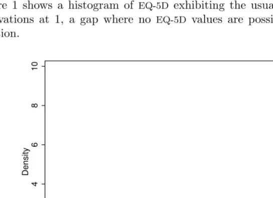
[image:8.612.128.400.327.524.2]

We now show how to use thealdvmmcommand to modelEQ-5Ddata. We useUKtariff data from the Patient Reported Outcome Measures in England, April 2011 to March 2012 (Health and Social Care Information Centre). The data are freely available and can be downloaded from http://www.hscic.gov.uk/catalogue/PUB11359. For this example, we select a 30% random sample of individuals with data on age and gender (age and gender are excluded from the dataset for those patients who could be identified because of low numbers). We use postoperative data on EQ-5D and the Oxford hip score of patients who have undergone a hip replacement. The Oxford hip score questionnaire combines a patient’s answers to 12 multiple-choice questions relevant to hips into one score, and it is designed to assess symptoms and function in patients undergoing hip replacements. Each question has 4 possible response categories; a score of 4 is assigned to the category representing the least or no symptoms, and a score of 0 is attached to the category representing symptoms of the greatest severity. The individual scores are then added together to one score with 0 denoting the worst possible symptoms and function and 48 denoting the best. Further details of the dataset can be found in Wineberg (2014).

Figure 1 shows a histogram of EQ-5D exhibiting the usual characteristics: a mass of observations at 1, a gap where no EQ-5D values are possible, and then a bimodal distribution.

0

2

4

6

8

10

Density

−.5 0 .5 1

EQ−5D index

Figure 1. Histogram ofEQ-5Ddata

(9)

distribution, and kurtotic densities; in fact, they can generate an incredibly large num-ber of distributional shapes. It is important to emphasize that bimodality does not necessarily imply a model with two components. The optimal model might have three or possibly more components if the distribution presents asymmetries or peaks.

We recommend that readers become familiar with the idiosyncrasies of fitting mix-ture models (McLachlan and Peel 2000) before attempting to estimate one. We will briefly describe the two main issues that researchers are likely to encounter when trying to fit models ofEQ-5Ddata. One of the problems of fitting mixture models relates to the presence of several local maximums in the likelihood function. We cannot assume that by running the model and getting some estimated parameters, the consistent so-lution has been found. To identify the global maximizer, we need, at the very least, to try different sets of random starting values and to select the solution with the highest likelihood function. Alternatively, a global optimization algorithm such as simulated annealing can be used. Thealdvmmcommand can use Stas Kolenikov’ssimann()Mata function for simulated annealing. We recommend using this option when fitting only a few components because it could be time consuming and because it cannot restrict the parameter space. Another problem arises when estimating mixtures with different

σc across components: the likelihood function becomes unbounded as the variance of a component tends to zero. It is not a “real” problem (Aitkin 1997); rather, it is due to the inability of the normal distribution to characterize the likelihood when the variances tend to zero. In essence, as the variance of one component becomes very small, the com-ponent turns into a conditional probability mass. However, the likelihood contribution of that component becomes infinite in (4) because we are dividing by a very small num-ber. In this situation, we cannot trust the value of the likelihood. Usually, provided that certain regularity conditions are met, the consistent solution will correspond to a local maximizer. EQ-5Ddata usually have a mass of observations at one corresponding to individuals who are in full health and then have no immediately adjacent observa-tions. If we try to estimate a standard mixture of normal distributions, we will quickly encounter problems with unbounded likelihoods as the model tries to fit the mass of observations. The adaptation to the mixture of normals used by thealdvmmcommand ensures that the likelihood value is correct even if a component becomes a probability mass at one. However, as in the standard mixture of normals, the likelihood function of a model displaying a component with a near-zero variance in the interior of theEQ-5D range should not be relied upon for model selection.

(10)

. use ohr11_12.dta

. generate male = sex == 1 . generate hr10 = hr/10

. aldvmm eq5d hr10, ncomponents(2)

initial: log likelihood = -14123.606

(output omitted)

Iteration 14: log likelihood = -577.37808

2 component Adjusted Limited Dependent Variable Mixture Model

Number of obs = 10,565

Wald chi2(1) = .

Log likelihood = -577.37808 Prob > chi2 = .

eq5d Coef. Std. Err. z P>|z| [95% Conf. Interval]

Comp_1

hr10 .2307964 .0022443 102.84 0.000 .2263977 .2351951

_cons -.0883435 .0083791 -10.54 0.000 -.1047663 -.0719208

Comp_2

hr10 885120.8 . . . . .

_cons 3930876 . . . . .

Prob_C1

_cons 7.320611 .731422 10.01 0.000 5.88705 8.754171

/lns_1 -1.646109 .0089019 -184.92 0.000 -1.663556 -1.628661

/lns_2 -164.8187 . . . . .

sigma1 .1927987 .0017163 .189464 .196192

sigma2 2.63e-72 . . .

pi1 .9993387 .0004834 .9972325 .9998422

pi2 .0006613 .0004834 .0001578 .0027675

(11)

. matrix a = e(b)

. constraint 1 [Comp_2]:hr10 = 0 . constraint 2 [Comp_2]:_cons = 100 . constraint 3 [lns_2]:_cons = 1e-30

. aldvmm eq5d hr10, ncomponents(2) from(a) constraints(1 2 3)

rescale: log likelihood = -577.37808

rescale eq: log likelihood = -577.37808

Wald chi2(1) = 10575.71

Log likelihood = -577.37808 Prob > chi2 = 0.0000

( 1) [Comp_2]hr10 = 0

( 2) [Comp_2]_cons = 100

( 3) [lns_2]_cons = 1.00e-30

Comp_1

hr10 .2307964 .0022443 102.84 0.000 .2263977 .2351951

_cons -.0883435 .0083791 -10.54 0.000 -.1047663 -.0719208

Comp_2

hr10 0 (omitted)

_cons 100 (constrained)

Prob_C1

_cons 7.320611 .731422 10.01 0.000 5.88705 8.754171

/lns_1 -1.646109 .0089019 -184.92 0.000 -1.663556 -1.628661

/lns_2 1.00e-30 (constrained)

sigma1 .1927987 .0017163 .189464 .196192

sigma2 1 (constrained)

pi1 .9993387 .0004834 .9972325 .9998422

pi2 .0006613 .0004834 .0001578 .0027675

(12)

. aldvmm eq5d hr10, ncomponents(2) inimethod(cons) Fitting constant-only model:

(output omitted)

Fitting full model:

(output omitted)

Iteration 15: log likelihood = 685.78629

LR chi2(2) = 8847.34

Log likelihood = 685.78629 Prob > chi2 = 0.0000

Comp_1

hr10 .3050275 .0063324 48.17 0.000 .2926162 .3174389

_cons -.4029312 .0215507 -18.70 0.000 -.4451698 -.3606925

Comp_2

hr10 .1480158 .0019441 76.13 0.000 .1442053 .1518263

_cons .2261472 .0069948 32.33 0.000 .2124377 .2398566

Prob_C1

_cons -.7075574 .061444 -11.52 0.000 -.8279855 -.5871293

/lns_1 -1.263205 .0211453 -59.74 0.000 -1.304649 -1.221761

/lns_2 -2.45414 .0177415 -138.33 0.000 -2.488913 -2.419367

sigma1 .2827464 .0059788 .2712677 .2947107

sigma2 .0859371 .0015247 .0830002 .0889779

pi1 .3301388 .0135882 .3040712 .3572938

pi2 .6698612 .0135882 .6427062 .6959288

(13)

After fitting the model, we can store the model and the estimated parameters and usepredictto get the model predictions.

. estimates store c2consp . matrix start2lc=e(b) . predict predc, outcome(all) . summarize predc*

Variable Obs Mean Std. Dev. Min Max

predc 10,565 .7730816 .1789941 .0323573 .9445987

predc_y1 10,565 .7083382 .2454649 -.360848 .9236923

predc_y2 10,565 .8049902 .1467324 .2261472 .9549023

predc_p1 10,565 .3301388 0 .3301388 .3301388

predc_p2 10,565 .6698612 0 .6698612 .6698612

We use the optionoutcome(all)so that in addition to the individualEQ-5D predic-tions (predc), we get the predictions for each component (predc y1andpredc y2) and the predicted probabilities for each component (predc p1andpredc p2). Because this model has constant probabilities of component membership, predc p1 and predc p2

are the same for all individuals and correspond top1andp2reported in the estimation output. The means of the two components are located toward the top ofEQ-5D(0.7083 and 0.8050).

In many cases, it is likely that the probabilities of the components will vary with observable characteristics. The variables may or may not be different from those used in the individual components. For simplicity, here we augment the model to include the Oxford hip score in the probabilities of component membership. We use the parameters of the constant probability model as initial values for the coefficients.

. matrix start = start2lc[1,1..4] , 0, start2lc[1,5..7] . matrix list start

start[1,8]

Comp_1: Comp_1: Comp_2: Comp_2: Prob_C1:

hr10 _cons hr10 _cons c5 _cons

y1 .30502755 -.40293118 .14801581 .22614716 0 -.70755741

lns_1: lns_2:

_cons _cons

(14)

. aldvmm eq5d hr10, ncomponents(2) probabilities(hr10) from(start)

initial: log likelihood = 685.78629

(output omitted)

Iteration 10: log likelihood = 942.71143

Wald chi2(3) = 7759.92

Log likelihood = 942.71143 Prob > chi2 = 0.0000

Comp_1

hr10 .0887522 .0108455 8.18 0.000 .0674954 .110009

_cons .0129138 .0269556 0.48 0.632 -.0399183 .0657459

Comp_2

hr10 .1619008 .0019171 84.45 0.000 .1581433 .1656582

_cons .1763049 .0075321 23.41 0.000 .1615422 .1910675

Prob_C1

hr10 -1.395115 .0557792 -25.01 0.000 -1.50444 -1.28579

_cons 2.431909 .1748113 13.91 0.000 2.089285 2.774533

/lns_1 -1.319285 .0340906 -38.70 0.000 -1.386101 -1.252468

/lns_2 -2.271434 .012582 -180.53 0.000 -2.296095 -2.246774

sigma1 .2673265 .0091133 .2500484 .2857985

sigma2 .1031641 .001298 .1006511 .1057398

(15)

. estimates store c2varp . predict predv, outcome(all) . summarize predv*

Variable Obs Mean Std. Dev. Min Max

predv 10,565 .7687237 .1938134 .0271162 .9487147

predv_y1 10,565 .3523726 .0830315 .0140072 .4392129

predv_y2 10,565 .80352 .1552294 .1763049 .9558767

predv_p1 10,565 .0992993 .1502761 .013862 .9192284

predv_p2 10,565 .9007007 .1502761 .0807716 .986138

Information criteria can be displayed as usual:

. estimates stats *

Akaike´s information criterion and Bayesian information criterion

Model Obs ll(null) ll(model) df AIC BIC

c2consp 10,565 -3737.884 685.7863 7 -1357.573 -1306.715

c2varp 10,565 . 942.7114 8 -1869.423 -1811.3

Note: N=Obs used in calculating BIC; see [R] BIC note.

Tests such as the likelihood-ratio test can also be carried out as usual:

. lrtest c2varp c2consp

Likelihood-ratio test LR chi2(1) = 513.85

(Assumption: c2consp nested in c2varp) Prob > chi2 = 0.0000

The number of components can be increased further. Of course, the analyst must exercise judgment in determining the appropriate number of components. Likelihood-ratio tests cannot be used to test models with different numbers of components because they involve testing at the edge of the parameter space (σc = 0), which distorts the distribution of the statistic. The Bayesian information criterion has been proposed as a useful indicator of the number of appropriate components, but other approaches also exist (McLachlan and Peel 2000).

6 Acknowledgments

(16)

7 References

Aitkin, M. 1997. Contribution to the discussion of paper by S. Richardson and P. J. Green. Journal of the Royal Statistical Society, Series B 59: 764–768.

Dolan, P., C. Gudex, P. Kind, and A. Williams. 1995. A social tariff for EuroQol: Results from aUKpopulation survey. Discussion Paper No. 138, University of York, Centre for Health Economics. http://www.york.ac.uk/che/pdf/DP138.pdf.

Hern´andez Alava, M., A. Wailoo, F. Wolfe, and K. Michaud. 2013. The relationship betweenEQ-5D, HAQand pain in patients with rheumatoid arthritis. Rheumatology 52: 944–950.

. 2014. A comparison of direct and indirect methods for the estimation of health utilities from clinical outcomes. Medical Decision Making 34: 919–930.

Hern´andez Alava, M., A. J. Wailoo, and R. Ara. 2012. Tails from the peak district: Adjusted limited dependent variable mixture models of EQ-5D questionnaire health state utility values. Value in Health15: 550–561.

McLachlan, G., and D. Peel. 2000. Finite Mixture Models. New York: Wiley.

Shaw, J. W., J. A. Johnson, and S. J. Coons. 2005. USvaluation of theEQ-5D health states: Development and testing of the D1 valuation model. Medical Care 43: 203– 220.

Wineberg, A. 2014. Finalised Patient Reported Outcome Measures (PROMs) in England: April 2011 to March 2012, Version V2.0. Leeds, UK: Health and So-cial Care Information Centre. http://www.hscic.gov.uk/catalogue/PUB11359/final-proms-eng-apr11-mar12-fin-report-v2.pdf.

About the authors

M´onica Hern´andez Alava is an applied microeconometrician in the Health Economics and Decision Science section in ScHARR, University of Sheffield, Sheffield,UK.