Pattern Recognition Using Associative Memories

(1)

Pattern Recognition Using Associative Memories

Nathan John Burles

Submitted for the degree of Doctor of Philosophy

University of York

Department of Computer Science

(2)

(3)

Abstract

The human brain is extremely effective at performing pattern recognition, even in the

presence of noisy or distorted inputs. Artificial neural networks attempt to imitate the

structure of the brain, often with a view to mimicking its success. The binary correlation

matrix memory (CMM) is a particular type of neural network that is capable of learning

and recalling associations extremely quickly, as well as displaying a high storage capacity

and having the ability to generalise from patterns already learned. CMMs have been used

as a major component of larger architectures designed to solve a wide range of problems,

such as rule chaining, character recognition, or more general pattern recognition. It is

clear that the memory requirement of the CMMs will thus have a significant impact on

the scalability of such architectures.

A domain specific language for binary CMMs is developed, alongside an

implementa-tion that uses an efficient storage mechanism which allows memory usage to scale linearly

with the number of associations stored. An architecture for rule chaining is then examined

in detail, showing that the problem of scalability is indeed settled before identifying and

resolving a number of important limitations to its capabilities. Finally an architecture for

pattern recognition is investigated, and a memory efficient method to incorporate general

invariance into this architecture is presented—this is specifically tested with scale

invari-ance, although the mechanism can be used with other types of invariance such as skew or

(4)

(5)

List of Figures

2.1 A multilayer perceptron . . . 27

2.2 A Hopfield network with four neurons . . . 31

2.3 A binary correlation matrix memory . . . 35

2.4 A small binary CMM, represented as a matrix and a feed-forward neural network . . . 35

2.5 Three tensor products, given in both matrix form and tensor product rep-resentation . . . 39

2.6 A set of associations represented as a tree . . . 40

2.7 Circular convolution with vectors of length 3 . . . 45

2.8 Circular correlation with vectors of length 3 . . . 45

2.9 Example non-deterministic finite state automaton . . . 48

2.10 A CMM as a state machine . . . 49

2.11 Baum codes generated with n= 5, s= 2, p1 = 2, p2 = 3, demonstrating a potential issue distinguishing overlapping vectors . . . 49

2.12 A typical architecture of the Neocognitron . . . 51

2.13 Decomposition of part of a square into simple primitives . . . 53

2.14 The “Original Architecture” CANN module configuration . . . 56

3.1 An example of the Yale format . . . 64

3.2 An example of the binary Yale format . . . 64

3.3 An example of the hybrid format . . . 65

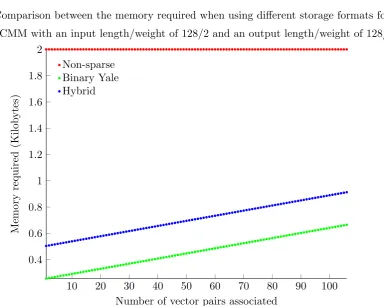
3.4 Scatter plots showing the memory requirements of a CMM using different storage formats, with short and long vectors . . . 68

(10)

3.6 Scatter plots showing the memory requirements of a CMM using different

storage formats, with different input and output vector weights . . . 71

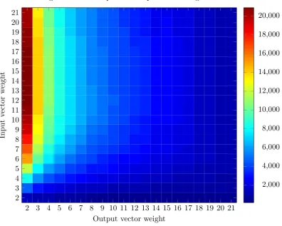
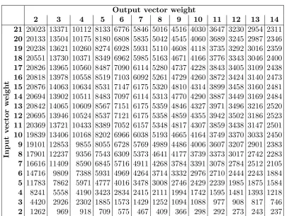
3.7 Heat map showing how the capacity of a CMM changes with vector weights 73

4.1 An example set of rules represented as a list and a tree . . . 78

4.2 Block diagram of ARCA . . . 80

4.3 A visualisation of the tensor product (b:r1)∨(c:r5) . . . 83

4.4 A visualisation of two iterations of the rule chaining process within ARCA . 84

4.5 Contour plots showing the recall performance of ARCA for branching

fac-tors 1 and 2 (non-sparse), plotting memory required against tree depth . . . 89

4.6 Contour plots showing the recall performance of ARCA for branching

fac-tors 1 and 2 (non-sparse), plotting memory required against number of rules 90

4.7 Scatter plots showing the recall performance of ARCA for branching factors

1 and 2 (non-sparse) . . . 92

3 and 4 (non-sparse) . . . 93

1 and 2 (binary Yale format) . . . 96

1 and 2 (hybrid format) . . . 97

4.11 Block diagram of the single CMM ARCA . . . 99

4.12 A visualisation of two iterations of the rule chaining process within the

single CMM ARCA . . . 101

4.13 Scatter plots showing the memory requirements of one- and two-CMM

ARCA for branching factors 1 and 2 . . . 104

ARCA for branching factors 3 and 4 . . . 105

ARCA for branching factor 1 with changing vector lengths . . . 107

ARCA for branching factor 2 with changing vector lengths . . . 108

4.17 Block diagram of multiple arity networks with ARCA . . . 111

(11)

LIST OF FIGURES

4.19 Scatter plots showing the memory requirements of ARCA with multiple

arity rules . . . 114

4.20 Scatter plots comparing the memory requirements of ARCA with single and multiple arity rules . . . 115

4.21 An example tree of rules, where only the path to be found is labelled . . . . 116

4.22 Mechanisms used in order to find the path between two nodes . . . 117

4.23 An English solitaire board . . . 119

4.24 Plots showing the number of operations required by a DFS to determine if a Solitaire state is valid or invalid, compared to the single operation ARCA requires . . . 121

4.25 Scatter plot comparing the number of operations required by a DFS to that required by ARCA to find a solution for a given state . . . 123

5.1 An example of the CANN recognising a simple shape . . . 128

5.2 The “Corner Turning 2” CANN module configuration . . . 129

5.3 Shapes to demonstrate the CANN’s arity network limitations . . . 132

5.4 The 8 patterns trained into the scale invariant CANN . . . 135

5.5 Feature extraction for the scale invariant CANN . . . 136

5.6 An example of the noisy inputs presented to the CANN for recall . . . 139

5.7 Plots showing the recall performance of the CANN with noisy inputs pre-sented at scales 25%–100% . . . 140

5.8 Plots showing the recall performance of the CANN with noisy inputs pre-sented at scales 125%–200% . . . 141

(12)

(13)

List of Tables

2.1 Example tokens, each allocated a binary vector generated using Baum’s

algorithm with n= 12, s= 2,p1= 5, p2 = 7 . . . 37

2.2 Baum codes generated withn= 12, s= 3,p1= 3, p2 = 4,p3 = 5 . . . 43

3.1 Simple operators available in ENAMeL . . . 60

3.2 Advanced operators available in ENAMeL . . . 61

3.3 Additional and compound operators available in ENAMeL . . . 62

3.4 The memory required to associate vector pairs in CMMs of varying size . . 69

3.5 Capacity of a CMM with independently varied input and output weights . . 74

4.1 A subset of the rules given in Figure 4.1, with a binary vector assigned to each individual vector and rule . . . 81

4.2 A set of rules to demonstrate the difficulty with multiple arity, with a binary vector assigned to each individual token vector . . . 110

5.1 Relaxation options for the CANN . . . 133

5.2 Recall results for the scale invariant CANN . . . 137

(14)

(15)

Acknowledgements

I wish to thank my supervisors, Jim Austin and Simon O’Keefe, for their invaluable

guidance, feedback, and support. I would also like to thank my assessors, Dimitar Kazakov

and Marc de Kamps, for giving up their valuable time to assist with this project. My

gratitude is extended to the Department and the EPSRC for providing financial support

for this research. Finally I would like to thank my mother, Tina, for help with

proof-reading this thesis, and most of all my wife Victoria, for her support and encouragement

(16)

(17)

Declaration

I declare that the research described in this thesis is original work, which I undertook at

the University of York during 2010 - 2014. Except where stated, all of the work contained

within this thesis represents the original contribution of the author.

Some of the material in Chapters 3, 4, and 5 have been previously published; where

items were published jointly with collaborators, the author of this thesis is responsible for

the material presented here.

• N. Burles, S. O’Keefe, and J. Austin. Incorporating scale invariance into the cellular associative neural network. In Artificial Neural Networks and Machine Learning–

ICANN 2014, pages 435–442. Springer, 2014

• N. Burles, S. O’Keefe, J. Austin, and S. Hobson. ENAMeL: A language for binary correlation matrix memories. Neural Processing Letters, 40(1):1–23, 2014

• N. Burles, S. O’Keefe, and J. Austin. Improving the associative rule chaining archi-tecture. In Artificial Neural Networks and Machine Learning–ICANN 2013, pages

98–105. Springer, 2013

• N. Burles, J. Austin, and S. O’Keefe. Extending the associative rule chaining archi-tecture for multiple arity rules. In Neural-Symbolic Learning and Reasoning

Work-shop, pages 47–51, Beijing, 5 August 2013

• J. Austin, S. Hobson, N. Burles, and S. O’Keefe. A rule chaining architecture using a correlation matrix memory. InArtificial Neural Networks and Machine Learning–

(18)

(19)

Chapter 1

Introduction

1.1 Motivation

Binary correlation matrix memories (CMMs) are a type of artificial neural network,

specifi-cally they are associative memories. They have been shown to have a high capacity, storing

a large number of associations between binary vectors [112], and their simplicity allows for

very fast storage and recall. CMMs have an ability togeneralise, to recall appropriate

asso-ciations when presented with an unseen input that is similar to known inputs, as well as to

perform correctly in the presence of noisy inputs. Binary CMMs, and architectures based

on them, have been effectively applied to problems in a wide range of domains, including

traffic management [53, 73], pattern recognition [16, 77], rule-based systems [9, 10], and

graph matching [62]. Although these architectures have been shown to be very capable,

some of them have a number of problems or limitations which reduce their applicability.

There are three main foci in this thesis. The first covers the problems which may

be encountered when attempting to incorporate binary CMMs into an architecture.

Al-though binary CMMs are capable of storing a large number of associations between input

and output vectors, their memory requirement is often unnecessarily high due to the use

of inefficient storage mechanisms—especially so when the CMM is not saturated.

Imple-menting CMMs efficiently, both in terms of memory and time, requires domain specific

knowledge that can act as a barrier for entry to the field. A simple implementation which

stores the matrices efficiently can greatly increase the scalability of architectures which

incorporate CMMs.

The second area focused upon is a rule-based architecture—the Associative Rule

(20)

given a starting state, and can be applied to any rule-based problem such as rule chaining.

It is limited, however, in terms of both applicability and memory requirement. As the

number of rules is increased the memory requirement increases exponentially, meaning

that the architecture will not scale to larger problems. In addition to this, all the rules in

a system must have the same arity—the same number of antecedents. Although this may

be sufficient in many cases, the ability to store multiple arity rules would be extremely

beneficial to allow the architecture to be applied to more complicated sets of rules or other

problems where the arity is likely to vary between rules, such as feature matching.

The final focus of this thesis is an architecture for distributed symbolic computation—

the Cellular Associative Neural Network (CANN). The CANN is another example of a

rule-based architecture, and is specifically applied to syntactic pattern recognition.

Pre-vious work has shown that the architecture is capable of performing pattern recognition

successfully [76], even in the case of noisy inputs and when using photographic images

rather than symbolically encoded data [16]. While the design of the CANN ensures that

it supports translation invariant pattern recognition innately, it is distinctly limited in its

suitability for this general task due to the lack of support for scale or rotation invariance.

A solution to incorporating general purpose invariance would enable the CANN to be

applied to a far wider range of pattern recognition problems.

The subject of this thesis is pattern recognition using rule-based CMM architectures,

aiming to develop and extend these architectures in order to enhance their suitability to

their respective applications. The project also aims to reduce the memory requirements

of CMMs in order to improve the scalability of any architectures using them, including

those designed for pattern recognition.

1.2 Thesis Summary

The previous section presented a brief discussion of the motivation behind this project. It

explained the limitations of two CMM-based architectures, and modifications or extensions

that are required in order that the architectures—and CMMs in general—may become

more suited to their intended purposes.

The overall aim of this project is to resolve the problems identified in the ARCA and

CANN systems, two architectures capable of performing rule-based pattern recognition.

Although these architectures have previously been shown to be sufficiently capable, the

(21)

1.2 Thesis Summary

and proficient for use with rule-based systems, demonstrating efficient memory usage and

potential to scale.

Below is a short list of any contributions made in this thesis:

• The development of a domain specific language for use with binary correlation matrix memories (Section 3.2), and an interpreter for this language that utilises an efficient

storage mechanism to allow large-scale simulations to be run (Section 3.3.2).

• An experimental analysis of the Associative Rule Chaining Architecture, comparing the memory requirement to the number of rules stored (Section 4.3.4), as well as when

changing the relative length of different vector types in the system (Section 4.4.3).

• Two methods to reduce the growth of memory required with respect to the number of rules from exponential to linear—using a sparse storage mechanism (Section 4.3.5)

and modifying the architecture (Section 4.4.3).

• Identification of a limitation of the “arity networks” proposed in previous work and provision of an alternative (Section 4.5) that has been tested experimentally—

allowing the Associative Rule Chaining Architecture to be successfully applied to

any directed acyclic graph or forest (Section 4.5.3).

• Demonstration that it is possible to find the path between two nodes using the Associative Rule Chaining Architecture, the first time this has been addressed

(Sec-tion 4.6).

• Application of the Associative Rule Chaining Architecture to a real problem, that of creating a Solitaire solver, providing a comparison between the number of operations

required by alternative methods of tree search (Section 4.7).

• Simplification of the architecture of the Cellular Associative Neural Network, in order that further improvements could be made (Section 5.3).

• Incorporation of a general purpose solution to handling invariance in the Cellular Associative Neural Network (Section 5.4), including a test of this applied to scale

invariance with symbolic images (Section 5.4.2), noisy images (Section 5.5), and

(22)

1.3 Chapter Overview

Chapter 2 begins with a discussion of associative memories, introducing some background

on artificial neural networks before presenting associationism and types of associative

memory—particularly the correlation matrix memory (CMM). Subsequently two

neural-network based architectures for object recognition are reviewed, presenting their salient

features as a means to reveal the motivations behind their development.

Chapter 3 introduces a domain specific language (DSL) for use with binary CMMs—

the Extended Neural Associative Memory Language (ENAMeL). This DSL is intended to

lower the requirements for entry to research using binary CMMs, as well as to provide

an efficient and scalable mechanism for storing binary CMMs. As such, following the

description of the language is an investigation of storage methods that may be employed.

In Chapter 4, a detailed description of a CMM-based architecture is given—the

As-sociative Rule Chaining Architecture (ARCA). The aim of ARCA is to be an efficient

method to perform forward chaining—inference of information by repeated application of

a set of rules to a state. More generically ARCA implements a tree search; whereas a

traditional method such as depth-first or breadth-first search looks at each node in turn,

ARCA inspects an entire layer of the tree simultaneously. After describing the existing

architecture, a number of important improvements are introduced. Firstly the use of an

efficient storage method in ENAMeL reduces the rate of growth of memory required, with

respect to the number of rules stored, from exponential to linear. The architecture is then

modified in order to reduce the memory requirements further. Notably this also reduces

the rate of memory growth from exponential to linear, in the event that the use of an

efficient storage mechanism is not possible. Next an extension to ARCA is introduced

which allows multiple arity rules to be successfully stored and recalled, before a method

is described to perform pathfinding using ARCA. Finally, ARCA is applied to the game

of Solitaire. This demonstrates that ARCA can successfully scale to large problems—in

this case 185.9M rules—and that the pathfinding method works correctly.

Chapter 5 focuses on another CMM-based architecture—the Cellular Associative

Neu-ral Network (CANN). This architecture was developed to perform translation-invariant

syntactic pattern recognition, using ideas from cellular automata. The CANN consists of

a network of simple processing cells, arranged in a regular grid, which in essence is overlaid

on an image. Each cell uses a small section of the image as its input, and by

(23)

1.3 Chapter Overview

performed hierarchically; tokens represent individual features within an image, and rules

combine them until an object is recognised. Rules are stored in CMMs in order to take

advantage of their speed during both training and recall, as well as to provide support

for partial matching in the case of distorted or occluded objects. While the CANN has

previously been shown to be effective, it is limited in its utility as it is not able to perform

scale or rotation invariant recognition. In order to introduce an extension allowing such

invariance the architecture is first modified to remove the “arity networks”. The

capa-bilities of the CANN are then augmented to allow invariant pattern recognition—this is

applied specifically to scale invariance, however the mechanism is suitable for adaptation

to other types of invariance such as rotation, skew, or stretch.

Finally, Chapter 6 conducts a review of the work presented in this thesis, discussing and

evaluating the degree to which the work completed meets the motivations of the project.

This chapter also combines any conclusions from the work presented throughout this thesis,

and draws any final and overarching conclusions from these. The thesis concludes with a

(24)

(25)

Chapter 2

Literature Review

2.1 Introduction

Traditional computing tends to place emphasis on obtaining the exact solution to a

prob-lem; neural networks are better suited to a “fuzzy” approach, finding an approximate

or good enough result. The cost of certainty and precision in some problems can be

large—they can become exponentially more difficult as the required precision increases.

An example given by Zadeh [116] is that of a human parking a car. With a large space to

park in, the problem is simple; as the space is reduced, or the required precision increased,

the difficulty of parking grows rapidly. As such, being imprecise can greatly reduce the

computation required to solve a problem, if the situation can tolerate some uncertainty.

Human cognitive abilities, such as understanding distorted speech and recognising

im-ages, stem from our ability to tolerate imprecision and uncertainty [116]. Pattern

recog-nition in particular is an area that is well suited to a brain-inspired approach—our ability

to recognise similar objects in different positions, invariant of scale and rotation, is due to

our ability to generalise.

In this chapter we first examine artificial neural networks, and in particular associative

memories. Following this we discuss distributed computation, and the use of a correlation

matrix memory as a state machine—a platform for symbolic computing. Finally, a number

of neural network-based architectures for pattern recognition are investigated. The work

reviewed in the following sections provides the background necessary to understand and

illustrate the limitations of current approaches, and the problems which this thesis has

(26)

2.2 Artificial Neural Networks

The human brain is incredibly complex, composed of around one hundred billion neurons

and many times more synapses [111]. These can be mapped during dissection to give a

good idea of the cellular and network structure of the brain. Alternatively, functional

magnetic resonance imaging (fMRI) can be used to determine the areas within the brain

that are used for particular tasks. These techniques do not tell us how the brain functions,

but in the connectionist approach it is assumed that since individual neurons are very basic

that the higher-level capabilities come from the structure.

Artificial Neural Networks (ANNs), often simply called neural networks, are systems

designed to mimic the structure of the brain. McCulloch and Pitts introduced simplified

neurons, as a model of biological neurons, in 1943 [68]. Research interest in ANNs grew

with the advent of back-propagation [89], as hardware development increased the size

and capabilities of these networks [65]. ANNs simulate the behaviour or structure of

animal brains, with many self-contained artificial neurons operating independently of each

other. Although ANNs are inspired by nature, they are not constrained by it and many

different types of ANN have been developed—some of these are designed as an attempt

to solve a specific problem, where others are an attempt to create a more general parallel

computation architecture.

There are many different types of neural network, generally separated into three classes

of learning—supervised learning, unsupervised learning, and reinforcement learning. Each

of these classes has particular types of problems to which it is better suited [59]. Supervised

learning requires pairs of input and output patterns to be presented to a network. The

network attempts to minimise the error between its own output and the expected output,

when presented with a particular input. In unsupervised learning, on the other hand, only

input patterns are presented. The network is provided with a cost function which it must

attempt to minimise—this function can be based on the input data and the network’s

output.

Reinforcement learning often uses a very different approach and explicit input or output

data may not presented at all, instead an agent learns from interactions with an

environ-ment. Numerical “rewards” denote the success of a particular action and an agent seeks to

maximise the reward obtained in the long-term. The cost associated with an interaction

(27)

2.2 Artificial Neural Networks

Input layer Hidden layer Output layer

(a)

i

j

Input

yj

xi

wij

xj

(b)

Figure 2.1: (a) A multilayer perceptron with a single hidden-layer and (b) inputs to a single neuron.

2.2.1 Feed-Forward Neural Networks

A feed-forward neural network is one of the simplest types of network to understand, and

is often employed for classification. The neurons are arranged in layers, and connections

must always go forward from a layer, creating a directed acyclic graph—there are no

connections that go backwards or between nodes within a layer [47].

The multilayer perceptron (MLP) is a commonly used feed-forward neural network,

able to distinguish linearly inseparable data. Each neuron in the network is a very simple

element, which takes one or more inputs, applies a function, and produces an output. An

example MLP is shown in Figure 2.1a, with a single “hidden” layer (a layer of neurons

which is not exposed as an input or output). Any function may be used in a neuron,

but the most common functions are linear, sigmoidal, or a simple threshold; in order to

distinguish linearly inseparable data the neuronal activation function of one or more layers

of neurons must be nonlinear [47].

As each of the neurons is independent of the others, it is possible for every neuron

to have a different function—during training, each of the parameters to this function can

then be gradually updated until the difference between the expected and actual output is

minimised. More commonly, every neuron in a layer will use the same, fixed function [92],

and instead the “weight” of a connection between two neurons is modified. The weight

of a connection is simply a factor by which the output of a neuron is multiplied before it

(28)

neuronj,yj, is thus:

yj =αj+

X

i

wijxi (2.1)

xj =f(yj) =f(αj+

X

i

wijxi) (2.2)

wherexi is the output of a neuroni,wij is the weight of the connection from neuron ito

neuronj, andαj is a constant offset or bias. The output of neuronj, orxj, is the result

of applying the neuron’s function toyj, as in Equation 2.2.

It is common for literature which introduces neural networks to discuss pattern

recog-nition, which may lead to a misapprehension that this is the only task to which neural

networks are applied. Although they are particularly well suited to it, they are not

lim-ited to this application and have been used in various fields including control, database

retrieval, and fault-tolerant computing [95].

The learning algorithm typically used with an MLP, error back-propagation, can limit

the practical use of these networks. The training period commonly occurs offline, meaning

the network is unavailable, and so this algorithm is not suitable for real-time

applica-tions [47]. Additionally it is possible for the back-propagation algorithm to become stuck

in alocal minimum, rather than finding theglobal minimum as is the aim [44,70]. Finally,

Tesauro and Janssens [102] showed an exponential relationship between the number of

neurons in an MLP’s input layer and the time required to train it. This demonstrated

a scaling problem—although MLPs have been successfully applied to small problems in

many areas, as problems grow larger they become computationally infeasible.

2.3 Associative Memories

In traditional computer memories, data is accessed using anaddress. This type of memory

is also known as a listing memory. Palm [80] defines a listing memory Ml as storing a

sequence of messages, where each message is a symbolstaken from an alphabet Σ:

Ml(Σ) = (s1, . . .,sn) :n∈N,s1, . . .,sn∈Σ (2.3)

(29)

2.3 Associative Memories

order to combine two sequences of messagesM and M0_{, they are simply concatenated:}

M = (s1, . . .,sn)

M0= (s01, . . .,s0k)

M+M0= (s1, . . .,sn,s01, . . .,s0k) (2.4)

Associative memories, or mapping memoriesMm, operate in a very different manner—

essentially they provide a system able to answer questions. Formally they are defined:

Mm(P, A) ={m:Q→A,Q⊆P,|Q|<|N|} (2.5) where a messagemis a mapping from a questionQto an answerA, andQis a finite subset

of the set of all possible questionsP. In this type of memory, messages are combined as

a set union—as long as the sets of questions are disjoint—with the answer to a question

q being provided by the appropriate mapping:

M =_{m:Q_→A_}

M0 =_{m0 :Q0 _→A0_}

(M+M0)(q) =

 



M(q) ifq_∈Q

M0(q) ifq_∈Q0

whereQ∩Q0 =∅ (2.6)

Stated more simply, a listing memory sequentially stores elements selected from an

alphabet and data is referenced directly by an address. An associative memory, on the

other hand, creates mappings between inputs and outputs—or questions and answers—

and data is referenced by the presentation of a known input causing the return of its

associated output.

Although their properties are very different, Palm [80] showed that it is trivial to

implement a mapping memory using a listing memory and vice versa. In order to store

mapped data in a listing memory, we can simply create a list where:

s1 =q1,s2 =a1, . . .,s2n−1 =qn,s2n=an (2.7)

and to implement a listing sequence in an associative memory we use the mapping:

(30)

While using a conventional listing memory to implement an associative memory in

this way is simple, it is also very slow and inefficient. In order to recall the output value

associated with an input qn, we must inspect the data stored at every address in turn

until we find the input and its associated output. Various methods, such as hashing [63],

may be used in order to improve upon this and reduce the number of memory accesses

required. Because the input must still be compared to that stored at a particular location,

however, a minimum of two memory accesses will always be needed—firstly to read the

input stored atsi and then to retrieve the output associated with this input fromsi+1.

A content addressable memory (CAM) is one that is designed to be fast for use with

mapping memories, storing data by value rather than by reference [1]. The simplest

implementation of this would be to use the binary value of an input as the address in which

to store the associated output. For example if we wanted to associate an input ‘2001’ with

an output ‘Kubrick’, we would store ‘Kubrick’ in address 2001 or 0b11111010001. It is clear that this method is not practical, however, as it is likely to lead to inefficient memory

utilisation and relies on input data having a binary representation that is short enough to

suitably use as an address. CAMs are therefore often implemented in specialised hardware

which searches the entire memory in parallel for a given input, and returns a list of all

outputs associated with it. Ternary CAMs provide a form of partial matching [79] by

introducing a value “don’t care” (X) in addition to the usual binary (0and1).

In general, however, both binary and ternary CAMs implemented using specialised

hardware are expensive and have a low capacity. As such, we will now investigate

alter-native methods based on artificial neural networks.

2.3.1 Hopfield Networks

Recurrent networks differ from feed-forward neural networks in that they form a directed

cyclic graph. They may contain feedback loops, which can be used to cause the network to

have astate—essentially a form of storage [88]. The Hopfield network, originally proposed

in 1982 [54], is one of the better known recurrent neural networks. Instead of having layers

of neurons like an MLP, every neuron in a network is connected to all of the others—

although some of the connections may have a weight of 0, which is equivalent to having

no connection.

Figure 2.2 shows an example Hopfield network with four neurons, in which the output

(31)

Inputs Outputs

Figure 2.2: A Hopfield network with four neurons

neuron may affect the input of every other neuron, these connections create feedback loops

that greatly increase the complexity of the network dynamics. Theenergy of a Hopfield

network,E, is calculated using Equation 2.9:

E=₋1 2

X

i,j

wijsisj−

X

i

iisi (2.9)

wherewij is the weight of the connection between neuronsiand j,si is the current state

of neuron i(a binary value), and ii is the value on the input to neuron i. Binary values

in this system can either be typical binary (0, 1) or bipolar (-1, 1). Typically Hopfield networks contain no self-connections, and all other connections are symmetric:

∀i:wii= 0 (2.10)

∀i, j :wij =wji (2.11)

Upon presentation of an input to the network, the activity of the neurons will gradually

update until the energy function has been minimised [54], this is then the final and stable

output state. In Hopfield’s original work the update function is asynchronous—a single

neuron is chosen at random, and its value is updated in order to minimise the energy of the

network. Hopfield networks can be updated synchronously, where all neurons are updated

simultaneously, however this is not biologically realistic as it requires a global clock [45].

One differentiating factor of these neural networks is that they are designed to continue

to run indefinitely; the outputs of a Hopfield network are influenced by the network’s

current state. In a feed-forward neural network an output is generated in direct response

to the presentation of an input, this means that changing the inputs will result in a series

of corresponding outputs—as the feed-forward network has no state, repeat presentation

of an input will always generate the same response. The Hopfield network, on the other

(32)

Due to the nature of the update operation, it is not designed to process a series of inputs—

with unstable inputs, the network may not reach a minimum before inputs are changed.

Additionally, the minimum reached with a given input may differ from one presentation to

the next as both the input and the current state of the neurons affect the next state. The

network continuously provides an output throughout its operation, which can potentially

give an estimation of a result as the optimisation is under way.

Training and operation of Hopfield networks are distinct, and so these networks are

required to be taken offline in order to train new information—depending on the

applica-tion this may be problematic. The training method is simple and fast, however, especially

when compared to error back-propagation [89]. They have, therefore, been successfully

used—particularly in pattern recognition (for example [75]), due to their ability to act as

a hetero-associative or auto-associative memory through careful training of the minima of

the network’s energy function.

The capacity of a Hopfield associative network has been studied rigorously in [69],

finding that under certain conditions the capacity is moderate. In contrast, however,

Baum et al. find that using a single layer matrix memory and a local representation can

result in a higher capacity [13]. One problem with Hopfield networks used in this fashion

that does not seem to have been adequately resolved stems from the nature of the recall

operation. For any given input, the network will continuously update until a minimum of

the energy function has been reached. There is the potential for the network to reach a

minimum that was not originally trained—although with careful training the probability

of this can be reduced.

Perhaps more interesting is the assumption that for any given input, a stable output is

desired. In alternatives, such as the Correlation Matrix Memory or Holographic Reduced

Representation that we will see later, presentation of an untrained input should result in

either an empty output, or an output with low confidence. Using a Hopfield network there

is no way to distinguish between items that have or have not been trained, or to determine

how much confidence should be assigned to the output.

2.3.2 Tensor Products

The concept of tensor products was introduced by Smolensky, described in detail in [96].

In this work, Smolensky discusses various vector representations: local, quasi-local, and

(33)

input neuron stores a single concept, and each concept is stored by only a single input

neuron. Local representations thus suffer from two limitations: they fail to efficiently

scale, as the number of input neurons increases with the number of concepts to be stored,

and the system may fail to operate if only a single neuron fails.

The quasi-local representation helps to resolve the second limitation of local

represen-tations, but at the expense of the first. In this case each neuron is used by only a single

concept, but a number of neurons represent each concept. In this way, multiple neuron

failures are required before the system will fail, however it multiplies the length of the

input and so compounds the problem of scaling. Finally, in a distributed representation

a concept is represented by the pattern of activity over a number of neurons. These

pat-terns may overlap, meaning that up to 2n patterns may be represented with onlynbinary neurons.

Smolensky [96] uses real-valued vectors and matrices, and presents two methods for

producing the matrix of associations—simple Hebbian learning, and a modified version

known as the “delta rule” which incorporates error-correction. Hebb [48] hypothesised

that:

When an axon of cell A is near enough to excite a cell B and repeatedly or

persistently takes part in firing it, some growth process or metabolic change

takes place in one or both cells such that A’s efficiency, as one of the cells firing

B, is increased.

In Hebbian learning the tensor product is found by calculating the outer product of

two vectors—that is to say that the value, or activation, of a neuron is set to the product of

its input and output activations. The superposition of two real-valued tensor products is

then found by using the sum operation. Using the delta rule, the activation of a neuron is

set to the product of its input activation and the difference between the output activation

and an expected value provided by an external teacher.

In the case that the vectors used are orthogonal, the two training methods produce

identical matrices [96]. Smolensky claims that the original Hebb’s method is therefore

somewhat limited—using the delta rule will result in a correct matrix for both local and

distributed representations, where Hebb’s method will only work correctly in local

rep-resentations (or a distributed representation where all the vectors have been carefully

selected to be orthogonal). Smolensky does not specify what is considered to be an

(34)

would produce the wrong result when a vector is recalled from it.

A particular problem with the use of tensor products in cognition is that the number of

matrix dimensions increases for every level of additional binding required, quickly causing

the tensor product to become too large to be feasible—biologically or otherwise—for all but

the smallest of problems [107]. It is argued (e.g. [43,99]) that this limitation can be avoided

through the use of reduced representations [49], such as convolution [84] (discussed further

in Section 2.3.6), elementwise multiplication [41, 60], or permutation-based thinning [87].

Jackendoff [58] presented four challenges for cognitive neuroscience, positing that the

connectionist approaches at the time—such as tensor products—failed to resolve the

prob-lems. Gayler [42] presented responses to each of these challenges, demonstrating that

Vec-tor Symbolic Architectures—a development of Smolensky’s tensor products—are able to

meet the challenges successfully. Further than this, Gayler emphasises that tensor product

networks are able to cope with The Problem of Variables. The productivity of language

leads to the difficulty that humans can generate and understand an infinite number of

sentences using a finite neural network. The use of variables allows for this

productiv-ity, assuming each variable may contain an arbitrary value [58]—allowing for complex

structures such as recursion.

In summary, although tensor products are relatively simple, they can be used to solve

certain sophisticated problems. Networks which make use of tensor products in more

com-plex architectures, or those which have developed from—and enhanced—tensor products,

have been shown to be capable of solving a range of complex challenges (e.g. [19, 20, 42]).

2.3.3 Correlation Matrix Memories

Correlation Matrix Memories (CMMs) and tensor products are very similar, both storing

the associations between pairs of vectors using the outer product. One distinction is

their intended purpose—CMMs are designed to be used as associative memories; tensor

products are intended to provide a distributed representation of a variable/value pair [97].

CMMs are thus a special type of feed-forward neural network that store associations

between pairs of vectors in a number of neurons, often represented as a matrix [64, 112].

They are a single layer, fully connected network, as every input neuron is directly connected

to every output neuron. Although CMMs may be “real-valued”—where the matrix of

connection weights may contain any real number—we are interested in a sub-class of

(35)

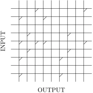
INPUT

[image:35.595.241.404.73.235.2]

OUTPUT

Figure 2.3: A binary correlation matrix memory

p q

r s

a

b

c d

(a)

b a

d c

Input layer Output layer

p q

r s

(b)

Figure 2.4: A small binary CMM, represented as (a) a matrix and (b) a feed-forward neural network. The neurons are labelled a–d, and the connections p–s. Neurons are generally not explicitly presented in matrix form, rather they are implicitly understood to be present.

Binary CMMs are a form of hetero-associative memory, or content-addressable

mem-ory [13]—information is recalled based on an association with input information, rather

than the knowledge of a particular storage location [74]. Depending on the content trained,

they can also act as an auto-associative memory—where the presentation of partial

infor-mation causes the recall of the complete inforinfor-mation, for example coping with occlusion

when performing pattern recognition [110].

Figure 2.3 shows an example binary CMM. Each horizontal line, or wire, represents

an input neuron, and each vertical wire an output neuron. This representation shows the

clear relationship between a CMM and its matrix—each intersection between wires is a

cell in the matrix of weights. In this binary CMM, a weight of 1 is marked, and a weight

of 0 is unmarked.

To aid comparison with other neural networks Figure 2.4 shows a very small (2×2)

binary CMM, firstly as a matrix and then as a feed-forward neural network. In these

(36)

between neurons have a weight of either 1 or 0, distributing an input or blocking the signal

respectively. The output neurons act in the manner common to perceptron networks, by

summing their inputs before applying a threshold.

A significant benefit of CMMs compared to many other neural networks is that they

may be trained while online, using high-speed, Hebbian learning. As mentioned earlier,

associations are formed using the outer product of input and output vectors; in a binary

CMM, tensor products can simply be superimposed onto an existing matrix using a logical

OR operation. The equation for training is formalised in Equation 2.12:

M=

n

_

i=1

xiyiT (2.12)

whereMis the resulting matrix of binary weights (the CMM),xis the set of input vectors,

yis the set of output vectors,nis the number of training pairs, andW

indicates the logical

OR of binary matrices.

Considering Smolensky’s claim that Hebbian learning is not suitable for use with

dis-tributed vectors, except if they are orthogonal, binary CMMs might be considered to

be somewhat limited when compared to real valued matrices. The delta rule cannot be

adapted for binary networks, as the activations of all neurons can only be set to either one

or zero—adjusting an activation to minimise error is simply not possible. In Willshaw’s

original work [112], however, it was demonstrated that using an appropriate threshold

method and value can overcome this apparent limitation and allow binary CMMs to

ef-fectively store a number of associations even with non-orthogonal vectors.

The recall process is similarly rapid, as shown in Equation 2.13. A non-binary vector

is first calculated by performing a matrix multiplication between the transposed input

vectorxT and the CMM M. A threshold functionf must then be applied to this vector, in order to produce the final binary output vector.

y=f(xTM) (2.13)

This recall operation may be greatly optimised, using the fact that the input vector

contains only binary components. For the jth _{bit in the output, the result of a matrix}

(37)

Token Binary vectorT Token Binary vectorT Token Binary vectorT

a 000100001000 e 000010000100 i 010000100000 b 000100100000 f 100000000010 j 000010010000 c 001000010000 g 010000000001 k 100000001000 d 100001000000 h 001001000000 l 100000100000

Table 2.1: An example set of tokens, with a fixed-weight binary vector allocated to each token. These binary vectors were generated using Baum’s algorithm [13] with a length of 12 and weight of 2 (with partition lengths 5 and 7), and assigned to the tokens randomly. The column vectors are shown here transposed for practical reasons.

of matrixM, represented asM[:,j]:

yj =xT ·M[:, j] (2.14)

The vector dot product is defined in Equation 2.15, where lis the input vector length

andMi,j is the value stored in the jth column of the ith row of matrix M.

yj = l

X

i=1

xiMi,j (2.15)

Given the binary nature of x, it is clear that this dot product is equal to the sum of all values Mi,j where xi = 1. The complete recall operation (without application of

a threshold) is thus formalised in Equation 2.16, where M[i,:] represents the ith _{row of}

matrixM:

y=

l

X

i=1

 



M[i,:] ifxi= 1

0 ifxi= 0

(2.16)

2.3.3.1 Tensor Product Representation

To describe the contents of a CMM or tensor product, without resorting to the use of

binary matrices, we use a pictorial representation. Using the example tokens given in

Table 2.1, the tensor product a : b1 _{is shown in Figure 2.5a. Below this matrix, in}

Figure 2.5d, is our higher-level representation of a tensor product—each displayed column

is labelled at the top with the input token it contains, and at the bottom with the output

token to which the input was bound.

Figures 2.5b and 2.5e show the result of superimposing this first tensor product with

1

(38)

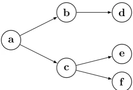
e:i. As there is overlap between the output vectorsb andi, the seventh column contains both vectors a and e superimposed. Finally, Figures 2.5c and 2.5f show a CMM trained with all of the associations in Figure 2.6. Although the matrix contains a large number

of trained vector pairs, in the pictorial representation it is still possible to quickly

deter-mine which columns contain a particular vector. Columns which are not displayed in a

tensor product are assumed to be filled entirely with zeros; it is possible that they contain

extraneous noise, however this is irrelevant for the purposes of the diagram.

2.3.4 Capacity of Correlation Matrix Memories

In [13], Baum et al. compared the capacity of an associative memory created using a

Hop-field network to the capacity of a binary CMM using a local representation. Quoting [69],

they state that in a Hopfield network with an input of lengthN, N/4 lnN pairs of vectors

may be associated while still allowing for correct recall.

In comparison, using a local representation stored in a binary CMM provides a capacity

that “is at least comparable to that of the Hopfield model” [13]. The lack of a definitive

capacity is due to the lack of fault-tolerance provided by a local representation—as only

a single neuron is used to represent each individual concept, if it were to fail then that

concept would be lost. In order to make the network more robust, the use of a quasi-local

representation is proposed—as long as every copy of a neuron does not fail, no content is

lost and the memory can be repaired.

Austin and Stonham [11] calculated a conservative estimate for the probability of recall

failure of a particular binary CMM trained with a number of associations to be:

P = 1−

 



1−

"

1−

1− N I

HR T#I

 



H

(2.17)

whereP is the probability of a recall failure (the recalled vector differs in some way from

the expected result),R andI are the length and weight of the input vector,H andN are

the length and weight of the output vector, andT is the number of pairs of vectors stored

in the matrix. Equation 2.17 says that as the “capacity” of an associative memory is

reached, when further associations are stored in the matrix, the probability of accurately

recalling any given vector will gradually decrease.

Turner and Austin [104] developed this further, creating a probabilistic framework

(39)

0 0 0 0 0 0 0 0 0 0 0 0 0 0 0 0 0 0 0 0 0 0 0 0 0 0 0 0 0 0 0 0 0 0 0 0 0 0 0 1 0 0 1 0 0 0 0 0 0 0 0 0 0 0 0 0 0 0 0 0 0 0 0 0 0 0 0 0 0 0 0 0 0 0 0 0 0 0 0 0 0 0 0 0 0 0 0 0 0 0 0 0 0 0 0 0 0 0 0 1 0 0 1 0 0 0 0 0 0 0 0 0 0 0 0 0 0 0 0 0 0 0 0 0 0 0 0 0 0 0 0 0 0 0 0 0 0 0 0 0 0 0 0 0

(a)

0 0 0 0 0 0 0 0 0 0 0 0 0 0 0 0 0 0 0 0 0 0 0 0 0 0 0 0 0 0 0 0 0 0 0 0 0 0 0 1 0 0 1 0 0 0 0 0 0 1 0 0 0 0 1 0 0 0 0 0 0 0 0 0 0 0 0 0 0 0 0 0 0 0 0 0 0 0 0 0 0 0 0 0 0 0 0 0 0 0 0 0 0 0 0 0 0 0 0 1 0 0 1 0 0 0 0 0 0 1 0 0 0 0 1 0 0 0 0 0 0 0 0 0 0 0 0 0 0 0 0 0 0 0 0 0 0 0 0 0 0 0 0 0

(b)

1 1 1 0 1 1 0 1 1 0 0 1 0 0 0 0 0 0 0 0 0 0 0 0 1 0 0 0 1 0 0 0 0 1 1 0 1 0 1 1 0 1 1 1 0 0 0 0 0 1 0 0 0 0 1 0 0 0 0 0 0 1 1 0 0 1 0 0 0 0 0 1 1 0 0 0 0 1 0 0 0 0 0 0 1 0 0 0 1 0 0 0 0 1 1 0 0 0 1 1 0 0 1 1 0 0 0 0 0 1 0 0 0 0 1 0 0 0 0 0 1 0 0 0 1 0 0 1 1 0 0 0 0 0 0 0 0 0 0 0 0 0 0 0

(c) b a b a d , f , k b ∨ c ∨ f (d) i e b a

b,i a_∨e

[image:39.595.121.522.163.517.2]

d , f , k b ∨ c ∨ f (e) d , f , k b ∨ c ∨ f g , i d ∨ e c , h a ∨ d b a e , j c ∨ f d , h b ∨ d b , i a ∨ e c , j a ∨ f k f e c f c g d (f)

(40)

a

b

c

d

e

f

g

h

i

j

k rab

rac

rbd

rce

rcf

rdg

rdh

rei

rf j

rf k

Figure 2.6: A set of associations represented as a tree, where the nodes represent vector tokens and the edges represent associations between them. In this tree the branching factor is 2, meaning that each node has at least one and at most two children.

any depth, as well as allowing for matching of partially presented inputs. A limitation

of all capacity estimations to date, however, is that they calculate the performance of

binary CMMs storing randomly-generated fixed-weight vectors. As we shall see in the

next sections, the capacity of a CMM is affected by the choice of threshold function and

increased significantly by increasing the orthogonality of vectors.

2.3.5 Threshold Functions

There are a number of functions which may be used as the threshold during a recall from

a binary CMM, although the choice of function may be limited by the application and

the data representation used. In a typical feed-forward neural network, the threshold can

be applied locally and independently in each individual output neuron. In a CMM there

may instead be a global function, applied to the values across all of the output neurons.

2.3.5.1 Willshaw’s Threshold

One of the simplest threshold functions isWillshaw’s threshold [112]. When training the

CMM, all input vectors are required to have the same fixed weight—the number of bits

set to1. During a recall, this fixed input weight is used as a simple threshold: any output neuron with a value greater than or equal to this weight is set to 1, and neurons with values below the limit are set to 0. When using this threshold with a complete input, the CMM is guaranteed to successfully recall all of the expected output bits. If a CMM

becomes saturated (with too many vector pairs associated in it) there may be additional

(41)

interactions and interference between similar patterns within the matrix.

Willshaw’s threshold allows for partial matching; relaxation is achieved by simply

reducing the threshold. For example if the fixed input weight is 4, then using a value

of 3 as the threshold will allow patterns missing a single input bit to be recognised.

Similarly, reducing the threshold further will allow recall with fewer correctly set input bits.

Reducing the threshold value can, however, have the negative side effect of increasing the

number of ghosts recalled—particularly if the matrix is approaching saturation. Without

employing relaxation the method will fail to recall if the presented input differs in any

way from that trained, meaning that it is susceptible to errors if recall inputs may be

noisy [11].

Finally, when using Willshaw’s method of thresholding, binary CMMs have the unusual

property of continuing to operate correctly when input vectors are superimposed [5]. The

resultant output vector then contains the superposition of the expected output vectors.

To illustrate this, consider the example set of vector tokens given in Table 2.1, and rules in

Figure 2.6. Figure 2.5c shows the matrix that results if these rules are trained into a CMM.

A recall of the vectorb (or 000100100000) results in an output of 201102110000. After applying Willshaw’s threshold with a value of 2 (the weight of an input vector), we recover

the vector100001000000—the expected vectord. Similarly, recallinge(or000010000100) results in an output of 020000200000, or 010000100000 after a threshold—again this is the expected vectori.

The superposition of these input vectors, b∨e, is 000110100100. The result of re-calling this from the CMM is 221102310000; it can be clearly seen that after applying the threshold, still using a value of 2, the vector110001100000contains the superposition of both of the expected outputs,d_∨i. Due to overlap between the vectors, however, all of the set bits that form vector l are present in the superimposed output. When using a distributed encoding, it is often not possible to determine which individual vectors are

actually present in a superimposed vector, and which simply appear to be present due to

overlap with other vectors.

2.3.5.2 L-max Threshold

An alternative threshold function is known as theL-max threshold [6]. In this case, when

training the CMM, all output vectors are required to have the same fixed weight. The

(42)

values to1and the rest to0—where lis the fixed weight of an output vector.

Austin and Stonham [11] showed that compared to Willshaw’s threshold this method

provides improved recall performance, and hence capacity, when presenting noisy input

vectors. It similarly provides an implicit ability for relaxation—by setting the highest

values to 1, the output values do not necessarily need to be as high as the weight of an input vector and so not all of the input bits need to be correctly set.

L-max suffers from one potential limitation—that an input may be associated with

only a single output—due to the requirement that l must be known. If an input vector

is individually associated with two output vectors, then the number of set bits in the

expected output cannot be determined. Similarly, input vectors cannot be superimposed

prior to a recall, aslis unknown.

2.3.5.3 L-wta Threshold

The final threshold function requires that vectors are generated using a specific algorithm,

known asBaum’s algorithm [13]. Baum et al. recognised that if the orthogonality between

vectors can be maximised, then the interference between pairs of stored vectors should be

minimised. To generate vectors of lengthn, and weights(where the weight of a vector is

the number of ones it contains), their algorithm is as follows.

Choose sco-prime numbers such that they sum tonand each number is greater than

the last:

p1 < p2 <· · ·< ps ,n= s

X

i=1

pi ,∀ij, i6=j⇒pi⊥pj

Every generated vector then contains a single “one” in the first p1 bits, another in the

next p2 bits, etc. As an example, with n = 12, s = 3, p1 = 3, p2 = 4, and p3 = 5, the

vectors—or codes—would be generated as shown in Table 2.2. Hobson [52] notes that the

requirement thatp1 < p2 <· · · is not strictly necessary, it is sufficient that the numbers

are all co-prime. Including the requirement in the algorithm does not lose any generality,

although it does not provide any benefit either.

Using the requirement, if only p1×p2 codes are generated, the minimum Hamming

distance between them will be 2s−2, as there will be at most a single 1 overlapping between any two codes. Similarly ifp1×p2×p3 codes are generated, there will be at most

two1s overlapping between two codes, giving a minimum Hamming distance of 2s−4 [13]. Without the monotonically increasing ordering, the same property holds—amending

(43)

1. 1 0 0 1 0 0 0 1 0 0 0 0

2. 0 1 0 0 1 0 0 0 1 0 0 0

3. 0 0 1 0 0 1 0 0 0 1 0 0

4. 1 0 0 0 0 0 1 0 0 0 1 0

5. 0 1 0 1 0 0 0 0 0 0 0 1

6. 0 0 1 0 1 0 0 1 0 0 0 0

..

. ... ... ... ... ... ... ... ... ... ... ...

Table 2.2: Baum codes generated with n= 12, s= 3,p1 = 3, p2= 4, p3 = 5

values. In general, if up to

t

Y

i=1

pi Baum codes are generated, for the smallest values of pi,

the minimum Hamming distance between any two codes will be 2(s₋t+ 1).

Baum et al. briefly mention the ability to exploit the known structure of the codes,

using a “winner takes all” approach to the threshold. This is developed by Hobson [52]

and termed theL-wta threshold. This method of thresholding is essentially an extension of

the L-max threshold—for each section of the recall result with lengthpi, L-max is applied

with anl-value of 1. Thus, in each of thessections the highest value is mapped to a one,

and everything else maps to zero.

Casasent and Telfer had previously experimented with the capacity of CMMs and

determined that, of those threshold methods they tried, using fixed-weight vectors and

the L-max threshold method allowed a CMM to have the highest capacity [23]. As such,

Hobson compared the storage capacity of a CMM when using L-max and L-wta. His

experimental results showed that when using Baum codes, the capacity achieved in a

CMM with the L-wta threshold is always the same or greater than that achieved with the

L-max threshold [52].

As the L-wta threshold is very similar to L-max, it suffers the same limitation: requiring

that l is known. For each of thes sections, the expected output is a single one, and so

output vectors cannot be superimposed—neither due to the superposition of input vectors,

nor association of a single input vector with multiple output vectors.

2.3.6 Alternatives to Tensor Products

One of the criticisms of tensor products is the potentially large amount of memory required

to store vector associations. Storing associations between two vectors of lengthsl and m

requires a matrix of sizel_×m. If a third vector is to be associated, of lengthn, then this

(44)

to store sparse matrices using a compressed representation, it is clear that the storage

requirements can increase rapidly for compositional structures, or for non-sparse codes.

Plate [84] proposes an alternative method of storing associated vectors. Rather than

simply using an outer product operation, associations are constructed using circular

convo-lution. The result of this operation is effectively a compressed form of the outer product, a

vector of the same length as those originally associated, known as the Holographic Reduced

Representation (HRR).

The general equation for circular convolution (~) is given in Equation 2.18 and shown

in Figure 2.7. The figure is an illustration of convolution applied to a pair of 3-bit vectors.

The 3×3 matrix is the outer product of vectors x and y, and vector z is the result of compressing—or convolving—this matrix [85].

z=x~y

zi= n−1

X

j=0

xjy(i−j) modn (2.18)

Under certain conditions, given an HRR storing only a single associated pair of vectors,

circular correlation (#) will work as the approximate inverse operation—performing a

recall operation to recover an associated vector, and giving a somewhat noisy result [84].

Equation 2.19 gives the general equation for this operation, and Figure 2.8 demonstrates

the process of reversing the previous circular convolution.

y≈z# x

yi ≈ n−1

X

j=0

z(i+j) modnxi (2.19)

In order to compose HRRs, Plate suggests simply adding them together. Having done

so, the recall operation will only work effectively to determine the presence of an associated

vector within the HRR, rather than to obtain the associated vector, due to the additional

noise that will be output. For a system using HRRs to be able to perform a full recall,

and actually retrieve the associated vectors, Plate proposed an additional stage after the

circular correlation—passing the retrieved vector through an auto-associative memory to

correct any errors.

Plate claims that “the exact method of implementation of the [auto-associative]

(45)

how-2.3 Associative Memories

x0

y0

z0

x1

y1

z1

x2

y2

z2

z=x~y

z0=x0y0+x1y2+x2y1

z1=x0y1+x1y0+x2y2

z2=x0y2+x1y1+x2y0

Figure 2.7: Circular convolution with vectors of length 3 (n= 3) [85]. Each of the circles is an element of the outer product of x and y. Each of the elements of the final circular convolution are sums along the diagonal lines.

z0

x0

y0

z1

x1

y1

z2

x2

y2

y≈z# x

y0 ≈z0x0+z1x1+z2x2

y1 ≈z0x2+z1x0+z2x1