A remarkably flat relationship between the average star formation rate
and AGN luminosity for distant X-ray AGN
F. Stanley,
1‹C. M. Harrison,
1D. M. Alexander,
1A. M. Swinbank,
1J. A. Aird,
1,2A. Del Moro,
1R. C. Hickox
3and J. R. Mullaney
41Centre for Extragalactic Astronomy, Department of Physics, Durham University, South Road, Durham DH1 3LE, UK 2Institute of Astronomy, University of Cambridge, Madingley Road, Cambridge CB3 0HA, UK
3Department of Physics and Astronomy, Dartmouth College, 6127 Wilder Laboratory, Hanover, NH 03755, USA 4Department of Physics & Astronomy, University of Sheffield, Hounsfield Road, Sheffield S3 7RH, UK
Accepted 2015 July 22. Received 2015 June 26; in original form 2015 February 25
A B S T R A C T
In this study, we investigate the relationship between the star formation rate (SFR) and AGN luminosity (LAGN) for∼2000 X-ray detected AGN. The AGN span over three orders
of magnitude in X-ray luminosity (1042 < L
2−8 keV<1045.5 erg s−1) and are in the redshift
rangez=0.2–2.5. Using infrared (IR) photometry (8–500 μm), including deblendedSpitzer
andHerschelimages and taking into account photometric upper limits, we decompose the IR spectral energy distributions into AGN and star formation components. Using the IR luminosities due to star formation, we investigate the average SFRs as a function of redshift and AGN luminosity. In agreement with previous studies, we find a strong evolution of the average SFR with redshift, tracking the observed evolution of the overall star-forming galaxy population. However, we find that the relationship between the average SFR and AGN luminosity is broadly flat at all redshifts and across all the AGN luminosities investigated; in comparison to previous studies, we find less scatter amongst the average SFRs across the wide range of AGN luminosities investigated. By comparing to empirical models, we argue that the observed flat relationship is due to short time-scale variations in AGN luminosity, driven by changes in the mass accretion rate, which wash out any underlying correlations between SFR andLAGN. Furthermore, we show that the exact form of the predicted relationship between
SFR and AGN luminosity (and its normalization) is highly sensitive to the assumed intrinsic Eddington ratio distribution.
Key words: galaxies: active – galaxies: evolution – infrared: galaxies – X-rays: galaxies.
1 I N T R O D U C T I O N
One of the key outstanding problems in studies of galaxy evolu-tion is understanding the connecevolu-tion between active galactic nuclei (AGN) and star formation. Both AGN activity and star formation are predominately dependent on the availability of a cold gas supply from the galaxy, as it is the fuel of both processes, and therefore a first-order connection between these two processes may be ex-pected. However, the scales of AGN activity and star formation are very different, which has lead to suggestions that any tight con-nection between them must be due to one process regulating the other (see Alexander & Hickox2012; Fabian2012; Kormendy & Ho2013for recent reviews).
E-mail:[email protected]
There are several pieces of empirical evidence for at least a broad connection between AGN activity and star formation. For example, the tight correlation observed between the mass of the supermassive black hole (SMBH) and the galaxy spheroid for galaxies in the local Universe (e.g. Kormendy & Richstone1995; Magorrian et al. 1998), serves as archaeological evidence of a connection between the growth of the SMBH (through mass accretion, where it becomes visible as AGN activity), and the growth of the galaxy (through star formation). Additionally, observations of AGN have found that the volume average of the SMBH mass accretion rate tracks that of the star formation rate (SFR), within∼3–4 orders of magnitude, up to redshifts ofz∼ 2 (e.g. Heckman et al.2004; Merloni, Rudnick & Di Matteo2004; Aird et al.2010) suggesting a co-evolution of AGN and star-forming activity. Despite how significant these results may appear, they only provide indirect evidence for a relationship between AGN activity and star formation and cannot place strong constraints on the form of the relationship.
C
To acquire more direct evidence on the form of the relationship between AGN activity and star formation requires sensitive mea-surements of the AGN and star-forming luminosities of individual galaxies. X-ray and far-infrared (FIR;λ=30–500 μm) observa-tions are ideal for quantifying the amount of AGN and star forma-tion activity, respectively. A key advantage of X-ray observaforma-tions, specifically in the hard band (e.g. 2–8 keV), over other tracers of AGN activity, is that they are not greatly affected by the presence of obscuration and contamination effects from the host galaxy (see sections 1 and 2 of Brandt & Alexander2015for more details of the use of the X-ray as an AGN tracer). A key advantage of FIR observations, as a measurement of star formation, is that they trace the peak of the obscured emission from star-forming regions sur-rounded by cold gas and dust. Even though the FIR provides an indirect tracer of star formation, a significant advantage over more direct tracers, such as the UV and optical emission from the young massive stars, is that it does not suffer significantly from obscura-tion (e.g. Kennicutt1998; Calzetti et al.2007; Calzetti et al.2010; see also section 2.2 in Lutz2014). Indeed, as shown by Dom´ınguez S´anchez et al. (2014), for luminous infrared galaxies (FIR lumi-nosities ofLFIR1044 erg s−1) more than 75 per cent of the total emission due to star formation is produced at FIR wavelengths, a fraction that increases at higherLFIR.1However, the AGN can also contribute to the FIR luminosity due to the thermal re-radiation of obscuring dust from the surrounding torus (e.g. Antonucci1993). Hence, for the most reliable measurements of the star formation it is important to apply decomposition methods of the AGN and star formation components at infrared wavelengths (e.g. Netzer et al. 2007; Mullaney et al.2011; Del Moro et al.2013; Delvecchio et al. 2014).
A number of studies have used X-ray and FIR observations to understand the connection between distant AGN activity and star formation by measuring the mean SFRs of AGN and star-forming galaxy samples (e.g. Lutz et al.2010; Shao et al.2010; Mainieri et al.2011; Harrison et al.2012; Mullaney et al.2012a; Rovilos et al.2012; Santini et al.2012; Rosario et al.2013a,b; Lanzuisi et al.2015). The main results shown by these studies are that: (1) the average star formation rates (SFR) of AGN track the increase with redshift found for the overall star-forming galaxy population; (2) theSFRof AGN are higher than those of the overall galaxy population (i.e. when including quiescent galaxies); and (3) the spe-cific SFRs (i.e. the ratio of SFR over stellar mass, which serves as a measure of the relative growth rate of the galaxy) of AGN are in quantitative agreement with those of star-forming galaxies. The majority of the current studies also find no correlation between the AGN luminosity andSFRfor moderate luminosity AGN (X-ray luminosities ofL2−8 keV1044 erg s−1; e.g. Lutz et al.2010; Shao et al.2010; Harrison et al.2012; Mullaney et al.2012a; Rovilos et al.2012). However, there are significant disagreements in the re-sults for high luminosity AGN (L2−8 keV1044 erg s−1). There are studies arguing that theSFRincreases at high AGN luminosities (e.g. Lutz et al.2010; Rovilos et al.2012; Santini et al.2012), a result that seems in agreement with the concept of AGN and star formation activity being connected due to their mutual dependence
1We note that for less luminous infrared galaxies (L
FIR1044 erg s−1), Dom´ınguez S´anchez et al. (2014) find that the FIR emission accounts for∼50 per cent of the total emission due to star formation. However in this work, we find that our galaxies have averageLFIR1044 erg s−1and so the majority of the star formation is expected to be produced at FIR wavelengths.
on the cold gas supply in the galaxy. Other studies have argued that the SFR decreases at high AGN luminosities (e.g. Page et al.2012; Barger et al.2015), potentially suggesting that the AGN may be responsible for reducing or even quenching the ongoing star forma-tion (a result also inferred by some simulaforma-tions of galaxy evoluforma-tion; e.g. Di Matteo, Springel & Hernquist2005; Hopkins et al.2005; Debuhr, Quataert & Ma2012). There are also studies arguing that
SFRremains constant up to high AGN luminosities (i.e. a broadly flat relationship; e.g. Harrison et al.2012; Rosario et al.2012; Azadi et al.2015), extending the trend seen for moderate luminosity AGN. Nevertheless, the difference in the conclusions of such studies could be attributed to the low source statistics for high-luminosity AGN, and strong field to field variations (e.g. Harrison et al.2012). For ex-ample, Harrison et al. (2012) demonstrated that when using a large high-luminosity AGN sample the broadly flat relationship between
SFRand AGN luminosity found for moderate luminosity AGN continues to high luminosities, with no clear evidence for either a positive or negative correlation (see also Harrison2014for a recent review).
To first order a flat relationship betweenSFRand AGN lumi-nosity can seem surprising, since it appears to suggest the lack of a connection between AGN activity and star formation. However, Hickox et al. (2014) have shown that a true underlying correla-tion between AGN luminosity andSFR can be masked if the AGN varies significantly (i.e. by more than an order of magni-tude) on much shorter time-scales than the star formation across the galaxy. In fact, observational studies such as Rafferty et al. (2011), Mullaney et al. (2012b), Chen et al. (2013), Delvecchio et al. (2014), and Rodighiero et al. (2015) have shown that when the average AGN luminosity is calculated as a function of SFR (i.e. taking the aver-age of the more variable quantity as a function of the more stable quantity) a positive relationship is found, suggesting that AGN ac-tivity and star formation are correlated on long time-scales. Studies using small-scale hydrodynamical simulations of SMBH growth (e.g. Gabor & Bournaud2013; Volonteri et al.2015) have indeed suggested that AGN activity can vary by a typical factor of∼100 over∼Myr time-scales, which results in a flat relationship between
SFRand AGN luminosity over a wide range of AGN luminosity. These studies therefore demonstrate that the relationship between AGN luminosity andSFRcan potentially place constraints on the variability of mass accretion on to the SMBH in galaxies. However, to date, the observational constraints of theSFRof AGN as a func-tion of AGN luminosity and redshift have lacked the accuracy to be able to distinguish between the different SMBH mass accretion models.
Most of the current studies on theSFRof distant X-ray AGN suffer from a variety of limitations, which affect the accuracy of
SFRmeasurements, such as: (1) small number of sources, which can lead to large statistical uncertainties, particularly at high AGN luminosities; (2) high levels of source confusion at FIR wavelengths, which can cause the overestimation of the flux; (3) use of a single FIR band from which to derive SFRs, which will result in large uncertainties on theSFRand will not take into account possible contamination of the SFR measurements from the AGN; (4) neglect of the information that can be obtained from the photometric upper limits of the FIR undetected AGN, which make up the majority of the distant AGN in X-ray samples (this final point is not applicable for studies that use stacking analyses).
and measure the SFR for each source in our sample. We use de-blended FIR photometry fromHerschel, which provides the best constraints on the FIR fluxes of individual sources by reducing the contamination due to blended and confused sources, the most significant drawback of theHerschelfield maps. Furthermore, we make use of the photometric upper limits in the fitting procedure to better constrain the SED templates and SFRs. We finally calculate theSFRvalues as a function of X-ray luminosity, with the in-clusion of sources with only upper limit constraints using survival analysis techniques (e.g. Feigelson & Nelson1985; Schmitt1985). Our methods ensure the use of all available data (i.e. photometric detections and upper limits, SFR measurements and upper limits) to provide improvedSFRas a function of X-ray luminosity and redshift. In Section 2, we outline the photometric catalogues used in this work, as well as the choice of redshift and the choice of matching radii between photometric positions. In Section 3, we analyse our methods of SED-fitting as well as the calculation of the average IR luminosity due to star formation (LIR,SF). Finally in Section 4, we present and discuss our results. In our analysis, we use H0=71km s−1,M=0.27,=0.73 and assume a Chabrier (2003) initial mass function (IMF).
2 AG N S A M P L E , I R P H OT O M E T RY A N D R E D S H I F T S
In this work, we use the available mid-IR (MIR;λ≈3–30) to far–IR (FIR;λ≈30-500 μm) photometric data to constrain the average SFRs of a large sample of X-ray detected AGN over the redshift rangez≈0.2–2.5. To construct a large sample of X-ray detected AGN we make use of three fields with deep X-ray observations: (1)ChandraDeep Field North (CDF-N; Alexander et al.2003b), (2)ChandraDeep Field South (CDF-S; Xue et al.2011), and (3) a combination ofChandra-COSMOS (C-COSMOS; Elvis et al. 2009) andXMM-COSMOS (Cappelluti et al.2009). To construct our final AGN sample, we obtain the MIR and FIR photometry from observations of the X-ray deep fields made with theSpitzer(Werner et al.2004) andHerschel(Pilbratt et al.2010) space observatories. The recentHerschel observational programmes PEP/GOODS-H
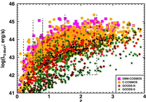
(Elbaz et al.2011; Lutz et al.2011) and HerMES (Oliver et al. 2012) in the three fields of GOODS-N, GOODS-S, and COSMOS, covering the wavelength range of 70–500μm are our main source of the FIR photometry (details in Section 2.2). We therefore restrict the CDF-N and CDF-S X-ray catalogues to these regions with sensitive MIR–FIR coverage, i.e. the GOODS-Nand GOODS-Swith areas of 187 arcmin2each, but use the full 2 deg2of COSMOS. In total, these areas cover 3609 X-ray sources. Fig.1shows the X-ray sources in GOODS-N, GOODS-S, C-COSMOS, andXMM-COSMOS in the L2−8 keV–zplane.
In the following subsections, we describe our sample selection and the catalogues used for the sample. In Section 2.1, we present the X-ray observations used to define our AGN sample and to determine their X-ray luminosities. In Section 2.2, we present the MIR and FIR photometric catalogues used to constrain the SFRs of the AGN hosts via SED fitting. In Section 2.3, we describe the method of matching the X-ray sources to the MIR and FIR catalogues and the redshift counterparts.
2.1 X-ray data
[image:3.595.309.548.55.222.2]To select the sample of AGN for our study, we use the publicly available X-ray catalogues for the CDF-N (Alexander et al.2003b), CDF-S (Xue et al.2010) and COSMOS (Cappelluti et al.2009; Elvis
Figure 1. X-ray (2–8 keV) luminosity (L2−8 keV) versus redshift (z) for the X-ray sources in the GOODS-N, GOODS-S, and COSMOS regions described in Section 2.1. Black centres indicate the X-ray sources without a direct hard-band detection (as described in Section 2.1). The vertical dashed lines indicate the four redshift ranges used in this study. The lower X-ray luminosity threshold (L2−8 keV>1042 erg s−1) used to define our AGN sample is shown with the horizontal dashed line. The combination of the three fields enables us to explore the SFRs of AGN over three orders of magnitude in AGN luminosity.
et al.2009) fields, restricted to the areas covered by
PEP/GOODS-Hand HerMES observations as described above (see Fig.1). For the COSMOS field, we use the C-COSMOS X-ray catalogue as the primary sample, while for the sources over the larger region, not covered byChandra, we use theXMM-COSMOS catalogue. Rest-frame, hard-band 2–8 keV luminosities were calculated following Alexander et al. (2003a) with the equation,
L2−8 keV=4π×D2L×F2−8keV×(1+z)(−2), (1) whereF2−8 keVis the observed X-ray hard-band flux (2–8 keV),DL is the luminosity distance,zis the redshift (see Section 2.3), and is the photon index used fork-corrections, which was fixed to a standard value of=1.9 (e.g. Nandra & Pounds1994). Although the hard-band observations in CDF-N and CDF-S are in the energy range of 2–8 keV, the C-COSMOS andXMM-COSMOS catalogues report hard-band fluxes of the energy range of 2–10 keV. To convert the 2–10 keV to 2–8 keV fluxes we assume=1.9 which yields a conversion factor of 0.85.
For the 20 per cent of X-ray sources in our final sample (see below) not detected in the hard band we used the full band of 0.5–8 keV (or the soft band of 0.5–2 keV if undetected in the full band) to estimate the hard-band flux. We estimated the hard-band flux assuming a = 1.4 spectral slope, unless this provided a measurement greater than the hard-band upper limit, in which case we assumed a=2.3 spectral slope; the assumed range in spectral slope is motivated by the range observed in AGN (e.g. Nandra & Pounds1994; George et al.2000). Overall, with this procedure, the hard-band fluxes were estimated assuming=1.4 for 19 per cent and=2.3 for 1 per cent of sources in our sample (see Fig.1).
2.2 Mid-IR & far-IR data
wavelength range of 8–500μm, provided by observations carried out by:Spitzer-IRAC at 8μm;Spitzer-IRS at 16μm;Spitzer-MIPS at 24μm, 70μm;Herschel-PACS at 70, 100, 160μm; andHerschel -SPIRE at 250, 350, 500μm. One of the advantages of our study over several previous studies, is the use of catalogues of deblended FIR
Herschelimages (details below). The deblending of sources in the PACS and SPIRE observations allows us to overcome the blending and confusion issues encountered in dense fields that can lead to an overestimation of the flux densities (e.g. Oliver et al. 2012; Magnelli et al.2013). It also ensures the direct association between the measured FIR flux densities and the sources used as priors in the deblending process. In addition to this, we also make sure that we have a reliable photometric upper limit for sources not detected in the FIR. This enables us to constrain the star-forming galaxy templates and gain an upper limit on the IR luminosity due to star formation, as we describe in Section 3.1.
The MIPS 24μm photometric catalogues that we use were cre-ated by Magnelli et al. (2013). These catalogues are made by si-multaneous point spread function fitting to the prior positions of 3.6μm sources. The catalogues were limited to a 3σdetection limit at 24μm going down to 20μJy in GOODS-Nand GOODS-S, and 50 μJy in COSMOS. The PACS 70, 100 and 160μm catalogues were also created by Magnelli et al. (2013) using the MIPS 24μm detected sources, described above, as the priors for the deblending of the PACS maps. Only sources with at least a 3σ detection at MIPS 24μm were used as priors and the resulting PACS catalogues were also limited to a 3σdetection limit.2The SPIRE 250, 350, and 500μm catalogues were created following the method described in Swinbank et al. (2014), again using these MIPS 24μm positions as priors to deblend the SPIRE maps.
Although both the PACS and SPIRE catalogues have been pro-duced in the same way, Magnelli et al. (2013) do not provide flux upper limits. In order to keep the priored FIR catalogues consistent with each other, we calculate upper limits for the non-detections in the PACS catalogues of Magnelli et al. (2013) in a similar way to the upper limit calculation performed for the SPIRE priored catalogues of Swinbank et al. (2014). This was done by performing aperture photometry at thousands of random positions in the PACS residual maps and taking the 99.7th percentile of the distribution of the mea-sured flux densities as the 3σupper limit on the non-detections. To account for the fact that the deblending is more uncertain in regions of luminous sources, we calculated these 3σupper limits as a func-tion of the pixel values in the original maps (see Swinbank et al. 2014). Consequently, this approach results in upper limits being higher for non-detected sources that lie near a bright source, when compared to non-detected sources in blank areas of the maps.
Due to the fact that we are using MIPS 24μm priored catalogues for the FIR photometry of our sources, any undetected at 24μm will not have FIR measurements in the published catalogues. Therefore for the 24μm undetected sources, we extracted the FIR photometry at the optical counterpart positions following the method described in Swinbank et al. (2014). Overall there are only 23 sources that are undetected at 24μm but have FIR counterparts, making up a very small fraction of our overall sample.
In the MIR bands, we also use the catalogues ofSpitzer–IRAC 8μm observations as described in Wang et al. (2010), Damen et al.
2The PACS catalogues for GOODS-Nand GOODS-Sare published in Magnelli et al. (2013). The catalogue for COSMOS was created in the same way and is available online (http://www.mpe.mpg.de/ir/Research/ PEP/DR1).
(2011), and Sanders et al. (2007), for GOODS-N, GOODS-S, and COSMOS, respectively, as well asSpitzer–IRS 16μm from Teplitz et al. (2011) for GOODS-Nand GOODS-S. Since all the IRAC catalogues have their detections determined by the 3.6μm maps, and the 16μm catalogues have been produced with the use of 3.6μm priors, they are all consistent with the deblended PACS and SPIRE catalogues described above.
2.3 Redshifts and catalogue matching
For our SED fitting analysis (see Section 3.1), we need matched catalogues containing X-ray fluxes, MIR-FIR photometric flux den-sities, and redshifts. To obtain the appropriate counterparts for each X-ray source, we matched the catalogues starting with the X-ray catalogues described in Section 2.1. We first match the positions of the optical counterparts of the X-ray sources to the MIPS 24μm positions in the catalogues of Magnelli et al. (2013).3To choose the matching radii between catalogues, we measure the number of total matches as a function of radius and estimate the fraction of spuri-ous matches for each matching radius. The matching radius of the X-ray to the MIPS 24μm catalogue for GOODS-Nand GOODS-S
was 0.8 arcsec, while for C-COSMOS andXMM-COSMOS it was 1 arcsec. This matching radius was chosen to maximize the num-ber of matches while minimizing the numnum-ber of spurious matches, with a ratio of spurious to true matches of 1 per cent. Due to the way that the FIR catalogues were deblended, each MIPS 24μm detected source also has a corresponding photometric measurement or flux upper limit for PACS 70, 100, 160μm and SPIRE 250, 350, 500μm (see Section 2.2). For the sources not matched to a MIPS 24μm counterpart, we use the FIR data extracted at their optical counterpart positions, as described in Section 2.2. We then match to the IRAC, and to the IRS 16μm catalogues for the two GOODS fields (see Section 2.2) using the same method.
A necessity for this analysis are the redshifts of the X-ray sources. To allocate the redshift counterpart of the sources in GOODS-Sand C-COSMOS we make use of the spectroscopic and photometric redshift compilation by Xue et al. (2011) and Civano et al. (2012), respectively. We also added redshifts from Teplitz et al. (2011) for sources in GOODS-Swhen necessary. For the sources in GOODS-N, we created our own compilation using catalogues of spectro-scopic redshifts from Barger et al. (2008) and Teplitz et al. (2011) and photometric redshifts from Wirth et al. (2004) and Pannella et al. (2009). Overall we obtained redshifts for 91.4 per cent of the X-ray sources.
In total, there are 3297 X-ray sources covered byChandra,XMM, and PEP/GOODS-Hobservations with a redshift (see Fig.1). For this study, we restrict this sample to redshifts ofz=0.2–2.5 and a luminosity range ofL2−8 keV>1042 erg s−1, resulting in our parent sample of 2139 AGN. Of the parent sample 53.3 per cent have spec-troscopic redshifts and 67.4 per cent are detected at MIPS-24μm (see Table1for a summary of the three fields).
3 DATA A N A LY S I S
In this study, we are interested in measuring the mean SFRs of galaxies, hosting an X-ray detected AGN, as a function of the AGN luminosity and redshift. We use multiband IR photometry, including
Table 1. Number of X-ray detected AGN in our parent sam-ple (L2−8 keV>1042erg s−1;z=0.2–2.5) in each field, as well as the number of sources with a spectroscopic redshift and the number of sources with a 24µm counterpart. Field AGN With spec-z With 24µm
GOODS-N 177 98 137
GOODS-S 209 128 154
COSMOS 1753 914 1151
Total 2139 1140 1442
photometric upper limits, to perform SED fitting for all 2139 X-ray detected AGN in our parent sample (see Section 2.3; Fig.1). For each source, we decompose the contribution of AGN activity and star formation to the overall SED. This allows us to measure the IR luminosity due to star formation (LIR,SF), the key quantity for this study, which we can use as a proxy for SFR (e.g. Kennicutt 1998; Calzetti et al.2007; Calzetti et al. 2010). In Section 3.1, we outline the SED fitting procedure and describe the calculation ofLIR,SF. In Section 3.2, we describe the method that we follow for the calculation of the averageLIR,SF as a function ofL2−8 keV (our tracer of the AGN luminosity) for the whole sample, where we include both directLIR,SFmeasurements and upper limits. The calculation of these values thus allows us to investigate how SFR relates to AGN luminosity (Section 4).
3.1 SED fitting procedure
To calculate individualLIR,SF values for our sample, we perform SED fitting to the MIR and FIR photometry. In these bands there
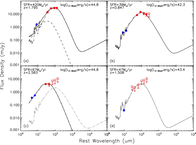
could be a contribution from both AGN and star formation, with emission from the AGN peaking at MIR wavelengths and dropping off at the FIR wavelengths (e.g. Netzer et al.2007; Mullaney et al. 2011). Those factors make it important to decompose the contribu-tion from both star formacontribu-tion and AGN to the overall SED so as to avoid an overestimation of the SFR measurement. In Fig.2, we give example SED fits to demonstrate our procedure.
To fit and decompose the IR SED of our sources, we develop the publicly availableDECOMPIRcode of Mullaney et al. (2011), and use the 8–500μm data and upper limits described in Section 2.2. We use a set of empirical templates that consist of the mean AGN template and the five star-forming galaxy templates originally de-fined in Mullaney et al. (2011), and extended by Del Moro et al. (2013) to cover the wide wavelength range of 3–105 μm. We also include the Arp220 galaxy template from Silva et al. (1998) which serves as a sixth template to ensure that we are also covering the possibility of extremely dusty star-forming systems. The advantage of using a few, but representative, templates to fit the data is that we can avoid the degeneracy in the fitting procedure caused by a large number of templates. Furthermore as many of our sources have lim-ited photometric detections (with only one or two data points), it is sensible to keep the number of free parameters as small as possi-ble. We note that the set of star-forming galaxy templates described above covers a broad range of empirical shapes, including the large template library of Chary & Elbaz (2001), as shown in fig. 2 of Del Moro et al. (2013), and the templates described by Kirkpatrick et al. (2012).
In our fitting procedure, the only free parameters of the fit are the normalization of the star-forming galaxy and AGN templates. Since there are two free parameters in the fit we require that the source has
[image:5.595.130.465.400.648.2]at least three photometric detections to simultaneously fit the AGN and star-forming galaxy templates. When we have less than three photometric detections we can only derive upper limits onLIR,SF, as we cannot constrain the AGN contribution (see below).
When a source is detected in three or more photometric bands, we perform a series of fits following the method of Del Moro et al. (2013). We fit the data in two steps: first, we fit using each of the six star-forming galaxy templates separately without including the AGN component, and secondly we fit again with each of the star-forming galaxy templates in combination with the AGN template. We fit to the photometric flux density detections, but use the avail-able flux density upper limits to eliminate the fits which are above any of the upper limits. This procedure results in a maximum of 12 models (the six star-forming galaxy templates without an AGN and the six star-forming galaxy templates with an AGN) to choose from.
To determine the best-fitting solution of the 12 possibilities de-scribed above, we use the Bayesian Information Criteria (BIC; Schwarz 1978) which allows the objective comparison of differ-ent non-nested models with a fixed data set, and is defined as
BIC= −2×lnL+k×lnN, (2)
where L is the maximum likelihood, k is the number of free pa-rameters, and N the number of data points. This method penalizes against models with extra free parameters counterbalancing the fact that a model with more free parameters can fit the data better, irre-spective of the relevance of the parameters. This is an improvement over a simpleχ2test or a maximum likelihood comparison that would tend to favour the model with more free parameters. For each source, the BIC value is calculated for all of the different fits. The best-fitting model will be the one which minimizes the BIC value, its absolute value being irrelevant; however for one model to be significantly better than the others it needs to have a difference in BIC value ofBIC≥2. IfBIC≤2 then both models are consid-ered equally valid (e.g. Liddle2004). Our final best-fitting solution is the one with the lowest BIC value; however, we only accept the AGN component as significant if the inclusion of it reduces the BIC value by≥2. In Fig. 2(a), we show a best-fitting SED that includes the AGN and star formation component, and in Fig.2(b) a best-fitting SED with only the star formation component. From the best-fitting SEDs, we then measure the integrated 8-1000 μm IR luminosity of the star formation component (LIR,SF). Further-more, if multiple fits have BIC values equal to the minimum BIC value, we consider them equally valid and take the average of their derivedLIR,SF.
For sources detected in fewer than three photometric bands, we can only calculate upper limits onLIR,SF, due to the insufficient degrees of freedom to calculate the AGN contribution to the IR luminosity. To calculate the upper limits of the normalization of each star-forming galaxy template, we increase the normalization of each template until it reaches one of the 3σupper limits, or exceeds the 3σuncertainty of a data point. We take the star-forming galaxy template with the highest upper limit ofLIR,SFas our conservative upper limit for that source (e.g. see Fig.2d). Using the same method, we also derive upper limits on the star formation contribution for sources where the best fit is fully dominated by the AGN (e.g. see Fig.2c).
Due to the limited photometry and quality of the data, our proce-dure is not expected to significantly detect an AGN component in the IR SEDs of all sources. Indeed, the detection of the AGN com-ponent in the MIR will be dependent on the relative ratio ofLIR,SF over the IR luminosity due to the AGN (LIR, AGN); for example, a
source with a high ratio ofLIR,SFoverLIR, AGNwill not show strong evidence of an AGN component in its IR SED (e.g. see appendix A of Del Moro et al.2013). However, we note that if we force an AGN component to be present in the IR SEDs of each of our sources, our results of mean LIR,SF in bins of X-ray luminosity and redshift (see Section 3.2) only change within a∼5 per cent level, which is smaller than the uncertainty of the meanLIR,SF results presented in Section 4.1. We also verified that our results were not sensitive to the choice of AGN template that we used. by refitting sources with two different AGN templates. One template is representative of low-luminosity AGN, while the other template is representative of high-luminosity AGN, as provided by Mullaney et al. (2011). The first template is ‘colder’ than that used in our main analysis, with less emission in the MIR and extended emission to the FIR wavelengths, and the second template is ‘hotter’, with most emission occurring at MIR wavelengths and a steep drop-off in the FIR (in agreement with the mean empirical templates of Quasars in the FIR; e.g. Netzer et al. 2007). Between them, these two templates, encompass most clumpy torus models (see fig. 7 in Mullaney et al.2011). In both cases, our results of meanLIR,SFin bins of X-ray luminosity and redshift (see Section 3.2) only change within a∼10 per cent level, which again is smaller than the uncertainty in the meanLIR,SFresults presented in Section 4.1.
Using our SED fitting approach, we have a sample of 2139 AGN with individual measurements (including upper limits) ofLIR,SF. From our results for the whole sample, there are 263 fits that required a significant AGN component in addition to star formation, 274 fits that required only the star-forming galaxy template, and for 1602 sources only upper limits on the star formation component could be derived due to limited photometry.
3.2 Calculating average source properties
For this study, we aim to constrain the average SFRs of our X-ray AGN sample as a function of redshift and X-X-ray luminosity. A challenge for all studies usingHerschelFIR photometry is the low detection rate of individual sources (e.g. Mullaney et al.2012a). In our sample, we can only place upper limit constraints on theLIR,SF for many of our sources, i.e. 1612 out of the 2139 (75.4 per cent) sources in our sample, due to the limited photometry or because they are AGN-dominated. In our study, we have placed conservative upper limits on theLIR,SFfor the AGN for which it was not possible to directly identify the star formation component (see Section 3.1). In order to not bias our study to only the FIR bright sources we study the average properties of the whole X-ray selected AGN sample by using a Survival Analysis technique (e.g. Feigelson & Nelson1985; Schmitt1985) to calculate the mean IR luminosities with the inclusion of all of the upper limits (details below).
of this method is that it does not assume an underlying distribution. We will refer to this method as the K-M method for the rest of this paper.
The main requirement for the use of the K-M method, is for the upper limit values to be randomly distributed among the measured values and independent of them. Due to the different types of up-per limits that result from our fitting procedure (see Section 3.1) the upper limits onLIR,SF are indeed random enough for the use of this method.4Furthermore, a K-S test on ourL
2−8 keV–zbins, with a probability threshold of 1 per cent, shows no evidence of the distributions of upper limits and measured values being drawn from different distributions. This method also requires that the lowest LIR,SFvalue in each bin is a measurement and not an upper limit. For the 12 bins where this is not the case, we follow the popu-lar procedure amongst studies using this method, and assume that the lowest value is a measurement (e.g. Feigelson & Nelson1985; Zhong & Hess2009). These 12 bins are randomly distributed with L2−8 keVand redshift (see Table2), and therefore do not affect our conclusions on the trends ofLIR,SFwith redshift, andL2−8 keV.
Feigelson & Nelson (1985) use the K-M method to estimate means with up to a censorship (i.e. the fraction of upper limits) of 90 per cent, but argue that there can be a significant bias in such cases. Additionally, a study by Zhong & Hess (2009) estimating the bias of this method for a wide range of distribution types, find that the estimated means are within a factor of 2 for up to 80– 90 per cent censorship levels. In our work, we have imposed a limit of 90 per cent censorship on our bins, and have discarded seven bins with greater censorship. The median censorship level amongst the remaining 45 bins we have used in our analysis is∼73 per cent, with 11 of them having a censorship of 80–90 per cent (see Table2). For the calculation of the uncertainty on the mean, we use the bootstrap technique, for which we take 10 000 random samplings in each bin and recalculate the mean. We then take the 16th and 84th percentiles of the overall distribution as the 1σerrors. As discussed above, bins of high censorship levels could suffer from additional uncertainties of a factor of2. However, when comparing to the results of the stacking procedure, we find that the two methods are consistent (see Appendix), and hence, we do not have concerns about the high censorship levels in our bins causing a significant systematic bias.
We show our final results ofLIR,SFas a function ofL2−8 keV in Fig.3. In our plots, throughout Section 4, we also include axes of SFR and AGN bolometric luminosity (LAGN) to help interpret the LIR,SF and L2−8 keV measurements. We calculate LAGN from L2−8 keVby using the luminosity dependent relation of Stern (2015) to convert theL2−8 keV to an AGN 6μm luminosity density. We then multiply this by a factor of 8 to convert the 6μm luminosity density toLAGN(following Richards et al.2006). The SFRs were calculated from theLIR,SFwith the use of the Kennicutt (1998) relation corrected to a Chabrier IMF (Chabrier2003).
4Our SED fitting procedure provides upper limits for the cases where a source is: (a) MIR–FIR undetected; (b) MIR–FIR detected, but in less than three bands; (c) AGN-dominated, i.e. the fit does not require any contribution from the SF templates. In the case of (a) the upper limits are calculated by constraining the SF templates to the flux upper limits, while in the cases of (b) and (c) they are calculated by constraining the SF templates to the 3σ flux errors or the flux upper limits. The fact that bright IR sources can meet the criteria of (b) and (c), in combination with the spatial dependence of the FIR flux upper limits, helps drive the similarity between the distributions of theLIR,SFupper limits and measurements.
4 R E S U LT S A N D D I S C U S S I O N
In this section, we present our results and explore the form of the relationship between the average SFR,LIR,SF, and X-ray lumi-nosity,L2−8 keV, for our sample of 2139 X-ray detected AGN (see Section 2). In Section 4.1, we present our results of average SFR (calculated fromLIR,SF) as a function of X-ray (and bolometric) AGN luminosity for four redshift ranges within z= 0.2–2.5. In Section 4.2, we compare the SFR of the AGN to those of the overall star-forming galaxy population, for a subsample of our sources with reliable host-galaxy masses. In Section 4.3, we compare our results to the predictions from two empirical models that connect AGN activity to star formation.
4.1 Mean SFR as a function of X-ray luminosity
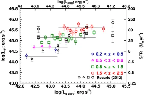
The main focus of this paper is to determine the form of the re-lationship between the average SFR and AGN X-ray luminosity over four redshift ranges. The results of our analysis as described in Section 3.2 are presented in Fig.3and Table2. In Fig. 3, the data are colour coded by redshift where each point is the mean of
≈40 sources and the error bars correspond to the 1σ of the boot-strap errors (see Section 3.2). We find that theLIR,SF(and hence SFR) increases with redshift, by a factor of∼3 between each red-shift range, in agreement with both the observed evolution found for normal star-forming galaxies (e.g. Elbaz et al.2011; Schreiber et al.2015) and previous studies on AGN populations (e.g. Shao et al.2010; Mullaney et al.2012a; Rosario et al.2012; Rovilos et al. 2012). However for the individual redshift ranges, we find no strong correlation betweenLIR,SFandL2−8 keV, a result inconsistent with that suggested by some other studies which have reported a rise or fall ofLIR,SFat high X-ray luminosities (e.g. Lutz et al.2010; Page et al.2012; Rovilos et al.2012; although see Harrison et al. 2012).
We find that our results are in general agreement to those stud-ies that stack the FIR data to derive SFRs using large numbers of sources (e.g. Harrison et al.2012; Rosario et al.2012); however, our results have reduced scatter and reduced uncertainties on the AGN contribution to the IR luminosity. We look in more detail at how our results compare to those of stacking in the appendix of this paper. Additionally, we compare our results directly to those of Rosario et al. (2012), who explore the average 60μm luminosity (νL60µm) values (as a tracer of SFR) in the same redshift ranges as our study, by stackingHerschel–PACS data. We use the average difference betweenνL60µmandLIR,SFfrom our SED fitting results, LIR,SF/νL60µm=2.2, to convert the results of Rosario et al. (2012) toLIR,SF. In Fig.4, we plot our results in comparison to those of Rosario et al. (2012, hollow black symbols) and find broad agree-ment with our results both as a function of redshift andL2−8 keV, although we have moreL2−8 keVbins and our results show less scat-ter. To compare to the highestL2−8 keVbins of Rosario et al. (2012) at the redshift ranges ofz=0.8–1.5 and 1.5–2.5, we calculate the
LIR,SFfor the five highestL2−8 keVsources in our study in both of these redshift ranges (plotted in Fig.4with solid black symbols). We find that our highestL2−8 keVsources are in agreement with those of Rosario et al. (2012); however, due to the very small number of sources in these bins (5–23 sources across both studies), we do not interpret them any further.
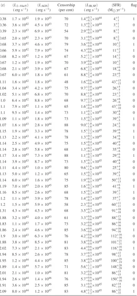
Table 2. The average redshift, X-ray luminosity, AGN bolometric luminosity, IR lumi-nosity due to star formation, and SFR, for the data presented in Fig.3. The errors on the
LIR,SFare calculated using the bootstrap analysis (see Section 3.2). We also provide the censorship level of each bin, and a flag indicating when the minimum value of the sources in that bin is an upper limit (when the flag has a value of 1), which can result to an extra uncertainty on theLIR,SF(see Section 3.2).
z L2−8 keV LAGN Censorship LIR,SF SFR flag ( erg s−1) ( erg s−1) (per cent) ( erg s−1) (M yr−1) 0.38 1.7×1042 1.9×1043 70 1.4+0.3
−0.3×1044 4+ 1
−1 1
0.36 3.6×1042 4.5×1043 72 1.3−+00..33×1044 3+ 1
−1 0
0.39 2.3×1043 6.9×1044 54 2.9+0.5
−0.5×10
44 8+1
−1 0
0.65 2.0×1042 2.3×1043 70 3.1+0.6
−0.7×1044 8+ 2
−2 0
0.68 3.7×1042 4.6×1043 79 3.6+0.8
−0.8×1044 10+ 2
−2 1
0.66 5.9×1042 7.9×1043 74 4.3+0.6
−0.6×1044 11+ 2
−2 1
0.68 8.2×1042 1.2×1044 67 5.2+1.1
−1.1×1044 14+ 3
−3 0
0.67 1.2×1043 1.9×1044 70 3.9+0.6
−0.6×1044 10+ 2
−2 0
0.68 2.1×1043 3.9×1044 67 6.8+2.2
−2.2×1044 18+ 6
−6 0
0.67 6.0×1043 1.8×1045 61 8.8+−22..44×1044 23+−67 0 1.11 1.6×1042 1.8×1043 48 1.6+0.6
−0.6×1045 43+ 15
−15 0
1.04 3.4×1042 4.2×1043 75 9.7+−22..00×1044 26+−55 0 1.02 5.1×1042 6.8×1043 70 8.8+−11..00×1044 23+−33 0
1.0 6.4×1042 8.8×1043 68 9.7+2.2
−2.3×1044 26+ 6
−6 0
1.1 7.9×1042 1.1×1044 65 1.6+0.4
−0.4×1045 43+ 10
−10 0
1.1 9.5×1042 1.4×1044 73 1.1+−00..33×1045 30+−88 0 1.09 1.1×1043 1.8×1044 73 1.5+−00..22×1045 39+−55 1 1.07 1.6×1043 2.8×1044 88 9.0+1.8
−1.8×1044 24+ 5
−5 0
1.15 1.9×1043 3.3×1044 78 1.5+−22..22×1045 39+−66 1 1.13 2.2×1043 4.1×1044 78 1.3+0.2
−0.2×1045 34+ 6
−6 1
1.14 2.5×1043 4.9×1044 75 1.5+0.4
−0.3×1045 40+ 9
−9 0
1.14 2.8×1043 5.8×1044 68 1.3+0.2
−0.2×1045 35+ 6
−6 0
1.17 3.4×1043 7.3×1044 88 1.1−+00..22×1045 29+ 6
−6 1
1.14 3.9×1043 8.7×1044 73 1.5+0.3
−0.3×1045 40+ 8
−8 0
1.11 4.4×1043 1.0×1045 80 9.6+1.6
−1.6×1044 25+ 4
−4 0
1.13 5.0×1043 1.2×1045 65 1.5+0.2
−0.2×1045 39+ 5
−5 0
1.14 6.0×1043 1.6×1045 75 1.9+0.5
−0.5×1045 50+ 13
−13 0
1.19 7.0×1043 2.0×1045 85 1.6+0.2
−0.2×1045 41+ 6
−6 1
1.16 8.5×1043 2.6×1045 68 1.5+−00..33×1045 39+−77 1 1.2 1.1×1044 3.9×1045 78 1.4+0.3
−0.3×1045 37+ 7
−7 0
1.2 1.5×1044 5.9×1045 58 2.3+0.4
−0.4×1045 60+ 11
−11 0
1.31 4.3×1044 4.5×1046 68 3.5+0.7
−0.7×1045 91+ 18
−18 0
1.88 3.2×1042 4.0×1043 61 3.3+−00..66×1045 88+−1516 0 1.83 1.1×1043 1.7×1044 73 3.2+0.6
−0.6×1045 86+ 16
−16 0
1.86 2.4×1043 4.6×1044 85 3.6+0.6
−0.6×1045 94+ 16
−16 1
1.9 3.0×1043 6.3×1044 76 4.2+0.6
−0.6×1045 112+ 16
−16 0 1.88 3.8×1043 8.5×1044 81 3.8+0.8
−0.8×1045 101+ 21
−21 0 2.02 7.3×1043 2.1×1045 83 4.4+0.6
−0.6×1045 116+ 16
−16 1 1.94 8.5×1043 2.6×1045 78 3.7+0.5
−0.5×1045 98+ 12
−12 0
1.95 1.2×1044 4.4×1045 85 3.8+0.9
−0.7×1045 100+ 25
−19 0 1.89 1.4×1044 5.7×1045 71 5.6+1.1
−1.1×1045 148+ 28
−29 0 2.01 2.1×1044 1.0×1046 81 3.2+0.6
−0.6×1045 86+ 15
−15 0
1.94 2.6×1044 1.4×1046 76 5.7+0.6
−0.6×1045 150+ 16
−16 0 1.91 3.6×1044 2.5×1046 85 3.1+0.5
−0.6×1045 82+ 14
−15 0
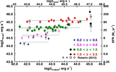
Figure 3. Mean IR luminosity due to star formation,LIR,SF, as a function of X-ray luminosity,L2−8 keV, for four redshift ranges. EachL2−8 keVbin has∼40 sources. We also give the corresponding SFR values using the Kennicutt (1998) relation corrected to a Chabrier IMF (Chabrier2003), and the bolometric AGN luminosityLAGNcalculated fromL2−8 keVusing the luminosity dependent relation of Stern (2015). The errors on theLIR,SFare calculated using the bootstrap analysis as described in Section 3.2 (see also Section 3.2 for a discussion on the additional uncertainties).
Figure 4. LIR,SFas a function ofL2−8 keV, as plotted in Fig.3(also to be referred to for axis definitions). The horizontal grey lines indicate the overall meanLIR,SFacross all of theL2−8 keVbins for each redshift range. The dashed grey lines indicate the meanLIR,SFfor (1) the one or two highest
L2−8 keVbins and (2) the lowerL2−8 keVbins for each redshift range (see Section 4.1). The black hollow symbols are the stacking results of Rosario et al. (2012), and the black filled symbols are bins of the highestL2−8 keV sources from our study (we note that there are very few sources in these bins for both studies; see Section 4.1). Our results are broadly consistent with a flat relationship; however, for the redshift ranges withz <1.5 the highest
L2−8 keVbins are systematically a factor of∼2 higher than the meanLIR,SF.
0.5< z <0.8 and 0.8< z <1.5, and by 0.4 dex (factor of 2.5) at the highest redshift range of 1.5< z <2.5. However, we note that the form of the observedflat relationshipofLIR,SFwithL2−8 keV (Fig.3) shows little to no change for all redshift ranges, in this extreme scenario.
To test whether our results are consistent with a flat trend of
LIR,SFwithL2−8 keV, we show in Fig.4, as a horizontal grey line, the meanLIR,SFfor each redshift range. Across all redshifts, the data lie within a factor of 2 of the mean. However, we find that the
LIR,SFvalues of the most luminous AGN for all of the redshift ranges atz <1.5 are systematically above the overall mean. To
quantify the deviation between theLIR,SFof the highL2−8 keVbins to the rest of the data we make two fits; one to the two highest L2−8 keVbins (with the exception ofz=0.2–0.5 where we use only the highestL2−8 keVbin); and one to the rest of the luminosity bins in the same redshift range (see the grey dashed lines of Fig.4). We find an increase inLIR,SFby a factor of∼2 for the highest L2−8 keV when compared to the lowerL2−8 keVbins in each of the redshift ranges withz <1.5. Forz=1.5–2.5, there is no significant difference inLIR,SFbetween the highest and lowestL2−8 keVthat we cover. We note that the systematic increase ofLIR,SFat high L2−8 keVvalues observed in the redshift ranges ofz <1.5 does not correspond to a systematic increase of the redshifts at highL2−8 keV values (see Table2). Thus, the modest trends observed at the high L2−8 keV are not driven by redshift. We investigate the observed trends further in Section 4.3.
4.2 Comparing to the average SFRs of the overall star-forming galaxy population
[image:9.595.48.287.326.474.2]Figure 5. LIR,SFas a function ofL2−8 keVfor the subsample of sources that have a reliable stellar mass (M∗) measurement in Ilbert et al. (2013, see Section 4.2; also see Fig.3for the axis definitions). The grey solid lines are the means for each redshift range of the whole parent sample (see Fig.4). The shaded regions correspond to the expected range inLIR,SFfor the overall star-forming galaxy population at the mean redshift and meanM∗ of each bin as defined by Schreiber et al. (2015). For all redshift ranges the
LIR,SFvalues of the AGN appear to be consistent with normal star-forming galaxies.
with a reliableM∗, we calculate theLIR,SFas described in Sec-tion 3.2. Due to the reduced number of sources with masses, we can no longer use bins of≈40 sources and we therefore reduce the number of sources required in each bin to 25. We show theLIR,SF as a function ofL2−8 keV, for the subsample with reliableM∗values, in Fig.5. We note that this subsample haveLIR,SFvalues consis-tent with the whole parent sample (see Fig.5), with the exception of thez=1.5–2.5 range which appear to be systematically higher. We use the mean redshift and meanM∗of each bin in Fig.5to calculate the expected range inLIR,SFfor ‘main-sequence’ galaxies using equation 9 of Schreiber et al. (2015). The shaded regions, colour-coded by redshift, correspond to the range of LIR,SF cov-ered by the main-sequence galaxies at the mean redshift and mean
M∗of the sources in each bin; i.e. a scatter of 2 around the mean results from Schreiber et al. (2015). We also find that these re-sults are the same if we use the Elbaz et al. (2011) definition of the ‘main sequence’. We find that, for this sample of X-ray AGN withL2−8 keV1044 erg s−1, theLIR,SFin all redshift ranges with z < 1.5 are consistent with that of star-forming galaxies of the same mean redshift and mass. This result agrees with the results of previous studies (e.g. Bongiorno et al. 2012; Harrison et al. 2012; Mullaney et al.2012a; Lanzuisi et al.2015). However, for the redshift range ofz=1.5–2.5, theLIR,SFis systematically at the higher end of theLIR,SF region covered by ‘main-sequence’ galaxies, which may be due, in part, to a bias due to the fact that only 26 per cent of the parent sample at those redshifts have reliable masses, and these have systematically higherLIR,SFvalues than the parent population (see Fig.5).
4.3 Comparing to empirical models
As shown in Fig. 4, the trend of LIR,SF(SFR) withL2−8 keV (LAGN) is broadly consistent with being flat. This result may ini-tially seem in disagreement with the results of studies such as Rafferty et al. (2011), Mullaney et al. (2012b), Chen et al. (2013), Delvecchio et al. (2014), and Rodighiero et al. (2015), which find a correlation between the averageLAGNand SFR of star-forming
Figure 6. The probability distribution of the Eddington ratio (λ) for the three cases assumed in Fig.7(i.e. two broken power-law distributions with a faint end slope ofα= −0.65 andα= −0.2, and a lognormal distribution with 0.4 dex dispersion; see section 2.2 in Aird et al.2013). This also serves as a schematic representation of the three distributions assumed for the Hickox et al. (2014) model, assuming that the shape of the distributions represent the variability function of individual AGN (see sections 4.3 and 2 of Hickox et al.2014).
galaxies. However, these studies start with a parent population of
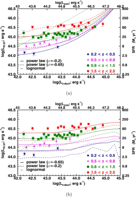
galaxiesfor which they calculate the averageLAGN, while in this study we start with a population of AGN for which we calculate the average SFR. It has been suggested that the variability of AGN, taking place on smaller time-scales to that of star formation, could flatten any intrinsic correlation between the SFR and theLAGNwhen not averaging over the most variable quantity (i.e. by taking the av-erageLAGNover bins of SFR; e.g. Hickox et al.2014). To assess what could be the driver of the flat relationship that we observe, and if indeed it is AGN variability that is driving its shape, we compare to two empirical ‘toy-models’ that predict theLIR,SFas a function ofLAGN. First that of Hickox et al. (2014) and secondly, a model based on Aird et al. (2013, also see Caplar, Lilly & Trakhtenbrot 2014, for a similar model).
The empirical ‘toy-model’ presented in Hickox et al. (2014) as-sumes that SFR is correlated toLAGNwhen averaged over time-scales of the order of 100 Myr. To create the SFR distribution of the galaxies in their model, they assume the redshift dependent IR lumi-nosity function (LF) from Gruppioni et al. (2013). In the model, the individual AGN are allowed to vary on short time-scales on the basis of an assumedLAGN/LAGNdistribution, which serves as a tracer of the Eddington ratio distribution of individual AGN in the absence of black hole masses (see details in Hickox et al.2014). The fiducial model assumes that the distribution ofLAGN/LAGNhas the form of a Schechter function (broken power-law form) with a faint end slope ofα= −0.2 and a cutoff luminosity ofLcut =100LAGN (see the dashed red curve in Fig.6for a schematic of this distri-bution). The model can then predict the average SFR as a function of instantaneous (i.e. observed)LAGNof a large population of sim-ulated AGN. We ran the model for the four redshift ranges of this study and plot the results in Fig.7(a) with solid tracks. The model successfully reproduces an increase of theLIR,SFwith redshift, for a fixed range inLAGN,5and is in good agreement with the data
5The increase of theL
[image:10.595.44.282.60.218.2]Figure 7. LIR,SFas a function ofL2−8 keVin four redshift ranges com-pared to model tracks from (a) Hickox et al. (2014) and (b) the extended Aird et al. (2013) model (see Fig.3for the axis definitions). The solid lines in both cases show the predictions of the models with their originally assumed Eddington ratio distribution. From the two models, the one of Aird et al. (2013), which is based solely on observational data, is in better agreement to our results; however both models demonstrate how the flatness of the trends in our results are likely to be a consequence of the assumed Eddington ratio distribution, or AGN variability. We also investigate how different the trends are when assuming different Eddington ratio distributions in the two models (i.e. two broken power-law distributions with a faint end slope ofα= −0.65 andα= −0.2, respectively, and a lognormal distribution for which we only show the tracks for 0.8<z <1.5 to avoid confusion; see Fig.6). The dif-ferent assumed Eddington ratio distributions show significant differences in the predicted trends. See Section 4.3 for more details.
atz=0.2–0.5; however, it fails to reproduce the trends observed for the higher redshift ranges. In particular, the normalization of the predicted trends are too low compared to our data and the rise of
LIR,SFwithLAGNis much steeper than that observed. The steep-ness of the predictedLIR,SFtrends at the highestLAGNcould be a result of the enforced correlation between SFR and the long-term
LAGN, or could be caused by the lack of an explicit Eddington limit
a correlation of SFR and the long-term-averagedLAGN. However, even though the increase ofLIR,SFwill be accompanied by an increase in the long-term-averagedLAGN, there is not a significant difference in the range of instantaneousLAGN, across the simulated population, which is the quantity we effectively observe for an X-ray AGN sample.
in the model but rather a cut-off limit at highLAGN/SFR ratios (see Hickox et al.2014for details). We investigate how the predicted relationship varies with different variability prescriptions later on in this section.
The second empirical ‘toy-model’ that we have compared to is based on Aird et al. (2013), which we extended to make predictions for the relationship between AGN luminosity and star formation. This model uses the observed redshift dependent stellar mass func-tion (SMF) of galaxies (from Moustakas et al.2013) in combination with the probability function of a galaxy of a given stellar mass and redshift hosting an AGN, based on measurements in Aird et al. (2012) for z 1. This model predicts the distribution of stellar masses, for which they correct to BH masses assumingMBH=0.002 ×M∗based on Marconi & Hunt (2003), as a function of X-ray lu-minosity. In contrast to the Hickox et al. (2014) model they use an Eddington ratio distribution in the form of a broken power-law function with the faint end slope being steeper withα= −0.65 (see the blue curve in Fig.6for a schematic of this distribution).6 In order to compare to our results, we have extended the model to cover the same redshift range as that of our sample and convert the predictions of stellar mass to predictions of SFR. To achieve this, we adopt the measurements of the SMF by Ilbert et al. (2013) at z=1–2.5 as an extension of the Moustakas et al. (2013) SMF up toz=1, and extrapolate the redshift-dependence of the probability of a galaxy hosting an AGN from Aird et al. (2012) toz >1 (which is consistent with thez >1 measurements from Bongiorno et al. 2012). Furthermore, we make the assumption that all of the AGN are hosted by normal star-forming galaxies that lie on the ‘main sequence’ as derived by Elbaz et al. (2011), which is motivated by the results of our study (see Section 4.2).7We convert from the model predicted stellar masses to SFRs, allowing for a scatter of 0.3 dex in SFR around the ‘main-sequence’ relation. In Fig.7(b), we present the resulting predictions ofLIR,SFas a function ofLAGN, plotted with solid lines, in comparison to our results for each of the four redshift ranges. The predicted trends of the mean SFR in this case are flat for a wide range ofLAGN, similar to our data, with a slight rise inLIR,SFat highLAGN(i.e.LAGN 1045 erg s−1). On the basis of this modified Aird et al. (2013) model, the slight rise ofLIR,SFobserved in our data (see Section 4.1) may be driven by a small increase in the average masses of the galaxies hosting very luminous AGN.
To first order, the data are better described by the extended Aird et al. (2013) model than the Hickox et al. (2014) model; see the solid tracks in Fig.7(b) compared to those in Fig.7(a). However, since the two models have assumed different Eddington ratio distributions (or, equivalently,LAGN/LAGNfor the Hickox et al.2014model), we also explore how sensitive the results are to this assumption. We therefore also ran the models with a series of three different Ed-dington ratio distributions to understand how sensitive the predicted trends ofLIR,SFwithLAGNare on the assumed Eddington ratio distribution. We used (1) a broken power-law withα= −0.2 (i.e. the fiducial distribution assumed by Hickox et al.2014); (2) a broken power-law withα= −0.65 (i.e. the fiducial distribution assumed
6We note that Aird et al. (2013) use an observed specific accretion rate distribution (i.e.LAGN/M∗) which they convert to an Eddington ratio dis-tribution.
by Aird et al.2013); and (3) a narrow lognormal distribution with a dispersion of∼0.4 dex centred at an Eddington ratio of∼0.06, as defined by Kauffmann & Heckman (2009) for nearby AGN residing in star-forming galaxies. These three distributions can be seen in Fig.6.
In Figs7(a) and (b), we show the three sets of tracks which correspond to the resulting trends ofLIR,SFwithLAGNfor the different assumptions of the Eddington ratio distributions. A clear correlation betweenLIR,SFandLAGNis predicted for the log-normal distribution while, by comparison, the power-law models predict a much flatter relationship. With a change of power-law slope fromα= −0.2 toα= −0.65, the normalization of the model tracks increase and the trend becomes flatter. The different shapes of the model tracks are driven by the relative difference between the low Eddington ratio slope and the slope of the low-mass end of the galaxy SMF (i.e. forM<M∗,α∼0). The predicted correlation betweenLIR,SFandLAGNfor the lognormal distribution is due to the narrow range of probable Eddington ratios. For the assumptions behind our models when assuming the lognormal distribution, most of the AGNs are accreting at a broadly similar Eddington ratio and therefore an increase inLAGNis predominantly due to an increase in stellar mass (and hence SFR since we assume the main sequence of star-forming galaxies). By contrast, the steep low-Eddington ratio slope for the power-law models, when compared to the low-mass end slope of the galaxy SMF, allows for a broad range of Eddington ratios across a narrow range in stellar mass; i.e. there is a higher probability for an AGN of a given luminosity to be hosted in a high-mass galaxy with a low Eddington ratio than a low-high-mass galaxy with a high Eddington ratio. Indeed, on the basis of the extended Aird et al. (2013) model, the population of low-to-moderate luminosity AGN (LAGN 1045 erg s−1) predominantly reside in galaxies of similar stellar mass (M∗ ∼1010.5–11M ), and thus similar SFRs, but with a wide range of possible Eddington ratios.
Overall, our results suggest that the observed trends ofSFR– LAGNare due to AGN being highly variable and residing, on aver-age, in normal star-forming galaxies. Similar results have also been found by hydrodynamical simulations that show that AGN variabil-ity can cause a flat trend betweenLAGNand SFR (e.g. Gabor & Bournaud2013; Volonteri et al.2015). The Eddington ratio distri-butions of AGNs are typically constructed to describe a population of AGN. However, as adopted in our models, they can also be under-stood as the distribution of Eddington ratios for an individual AGN over time, and hence could be used as a variability prescription of the AGN (as originally adopted in Hickox et al.2014). As is clear from Figs7(a) and (b), the choice of Eddington ratio distribution plays a major role in the form of the predictedSFR–LAGN rela-tionship. For example, our results are much better described with the use of a broken power-law Eddington ratio distribution with a faint end slope ofα= −0.65, than with a narrow lognormal Ed-dington ratio distribution, which predicts a qualitatively different
SFR–LAGN relationship to that found from our data. Thus, the SFR(orLIR,SF)–LAGNplane can be a useful diagnostic tool for placing constraints on the intrinsic Eddington ratio distribution of AGN (also see Veale, White & Conroy2014).
5 C O N C L U S I O N S
We have created a large sample of X-ray detected AGN with FIR coverage and individual SFR measurements. Our sample has a total of 2139 AGN at redshifts of z= 0.2–2.5, with 1042< L
2−8 keV< 1045.5 erg s−1. Using the available photometry from 8–500μm, we
have performed individual SED fitting to all of the sources in our sample, and measure the IR luminosity due to star formation,LIR,SF. Our analysis has a number of key advantages over many previ-ous studies: (a) the use of deblended source catalogues for the FIR photometry, which ensures better constraints on the flux density measurements and eliminates the overestimation due to blending and confusion of sources (see Section 2.2); (b) the use of photo-metric upper limits in the SED fitting analysis, which achieve better constraints on the fitted SEDs (see Section 3.1); (c) the decom-position of the AGN and star formation contributions to the FIR emission, which provides values ofLIR,SFthat are not contaminated by the AGN (see Section 3.1); (d) the calculation of upper limits onLIR,SFwhen the data are insufficient to identify the star-forming component directly (i.e. not enough photometric data points, poor S/N data, or dominant AGN component), which allows us to esti-mate theLIR,SFfor all the sources in our sample avoiding the bias that could be caused by removing these sources (see Section 3.2).
With the LIR,SF measurements for each source, we derived the meanLIR,SFvalues (LIR,SF; a proxy of theSFR) as a function ofL2−8 keV(a proxy of the AGN luminosity;LAGN) in bins of∼40 sources, for the redshift ranges of 0.2–0.5, 0.5–0.8, 0.8–1.5, and 1.5– 2.5. In comparison to previous studies, our results show less scatter amongstLIR,SFacross the wide range ofL2−8 keVinvestigated in this study. Overall we found that
(i) theSFRincreases by more than an order of magnitude from redshifts of 0.2–0.5 to 1.5–2.5, in agreement with previous studies on the redshift evolution of the SFR for the general star-forming galaxy population. See Section 4.1.
(ii) For each redshift range, theSFRshows no strong depen-dence on AGN luminosity; however, we note that for the redshift ranges ofz≤1.5 the highestLAGNsystems haveSFRvalues that are systematically higher than those of lowerLAGNsystems by a factor of≈2. See Section 4.1.
(iii) For the∼40 per cent of the sources within the COSMOS area with reliable stellar masses, we compare theirSFRto the ‘main sequence’ of the overall star-forming galaxy population. The X-ray AGN, at all redshift ranges, haveSFRthat are consistent with normal star-forming galaxies at the same redshifts and masses. Due to a lack of secure masses for the highLAGNsystems in our sample this result is restricted to moderate AGN luminosities (i.e.L2−8 keV
1044.2 erg s−1orL
AGN1045.5 erg s−1). See Section 4.2. (iv) To qualitatively understand the flat relationship between the
SFRandLAGN, we compared to two empirical ‘toy-models’ that make predictions for this relation: Hickox et al. (2014) and an ex-tended version of Aird et al. (2013). These models take mock galaxy populations and assign them with SFR values based on observed distributions, and instantaneousLAGNvalues based on an assumed Eddington ratio distribution. We find that the flat relationship seen in our data could be due to short time-scale variations in the mass accretion rates, which, in combination with the relative shapes of the Eddington ratio distribution and the galaxy SMF, can wash out the long-term relationship betweenSFRandLAGN. See Section 4.3