Tracking and diameter estimation of retinal vessels using Gaussian process and Radon transform

(1)

Gaussian process and Radon transform

.

White Rose Research Online URL for this paper:

http://eprints.whiterose.ac.uk/135023/

Version: Accepted Version

Article:

Asl, ME, Koohbanani, NA, Frangi, AF orcid.org/0000-0002-2675-528X et al. (1 more

author) (2017) Tracking and diameter estimation of retinal vessels using Gaussian process

and Radon transform. Journal of Medical Imaging, 4 (3). 034006. ISSN 2329-4302

https://doi.org/10.1117/1.JMI.4.3.034006

(c) 2017, Society of Photo-Optical Instrumentation Engineers (SPIE). This is an author

produced version of a paper published in the Journal of Medical Imaging. Uploaded in

accordance with the publisher's self-archiving policy.

[email protected] https://eprints.whiterose.ac.uk/

Reuse

Items deposited in White Rose Research Online are protected by copyright, with all rights reserved unless indicated otherwise. They may be downloaded and/or printed for private study, or other acts as permitted by national copyright laws. The publisher or other rights holders may allow further reproduction and re-use of the full text version. This is indicated by the licence information on the White Rose Research Online record for the item.

Takedown

If you consider content in White Rose Research Online to be in breach of UK law, please notify us by

(2)

Tracking and diameter estimation of retinal vessels

using Gaussian process and Radon transform

Masoud Elhami Asl,aNavid Alemi Koohbanani,aAlejandro F. Frangi,band Ali Gooyab,* a_{Tarbiat Modares University, Faculty of Electrical and Computer Engineering, Tehran, Iran}

b_{University of Sheffield, Centre for Computational Imaging and Simulation Technologies in Biomedicine,} Department of Electronic and Electrical Engineering, Sheffield, United Kingdom

Abstract. Extraction of blood vessels in retinal images is an important step for computer-aided diagnosis of ophthalmic pathologies. We propose an approach for blood vessel tracking and diameter estimation. We hypoth-esize that the curvature and the diameter of blood vessels are Gaussian processes (GPs). Local Radon trans-form, which is robust against noise, is subsequently used to compute the features and train the GPs. By learning the kernelized covariance matrix from training data, vessel direction and its diameter are estimated. In order to detect bifurcations, multiple GPs are used and the difference between their corresponding predicted directions is quantified. The combination of Radon features and GP results in a good performance in the presence of noise. The proposed method successfully deals with typically difficult cases such as bifurcations and central arterial reflex, and also tracks thin vessels with high accuracy. Experiments are conducted on the publicly available DRIVE, STARE, CHASEDB1, and high-resolution fundus databases evaluating sensitivity, specificity, and Matthew’s correlation coefficient (MCC). Experimental results on these datasets show that the proposed method reaches an average sensitivity of 75.67%, specificity of 97.46%, and MCC of 72.18% which is comparable to the state-of-the-art.©2017 Society of Photo-Optical Instrumentation Engineers (SPIE)[DOI:10.1117/1.JMI.4.XX.XXXXXX]

Keywords: diameter estimation; Gaussian process; Radon transform; retinal imaging; vessel tracking. Paper 17019RR received Jan. 24, 2017; accepted for publication Aug. 9, 2017.

1 Introduction

Analysis of vascular structures in retinal images can be impor-tant for diagnosis of several pathologies related to diabetes, cardiovascular disorders, and hypertension.1,2_{For instance,}

dia-betic retinopathy can be detected early by examining morpho-logical variations in vasculatures, preventing vision loss and blindness.3–5 _{To quantify these complications, accurate retinal} vessel detection and diameter estimation are often required.6 Generally, semiautomatic or automatic vessel segmentation tools are preferred over manual delineation, because the latter is difficult and user-dependent. However, due to imaging imper-fections and noise, accurate delineation imposes a special chal-lenge on nonmanual methods, particularly when thin vessels are of concern.7

A wide range of vessel extraction methods from medical images has been proposed in the literature. Interested readers are referred to Patton et al.,8Lesage et al.,9Mookiah et al.,10 and Fraz et al.11for detailed reviews. However, each method only excels in a few particular quality aspects such as computa-tional load, robustness to variation of region of interest, and im-aging modality. The performance of vessel segmentation methods can usually be improved by a preprocessing step.12 The aim of this stage is to intensify valuable information and eliminate noise, which could otherwise adversely affect the final outcome. Different methods have been proposed for this purpose.13,14_{Even though a preprocessing step could improve}

segmentation, it can lead to loss of important features, particu-larly at edges and narrow vessels. Therefore, despite some

relative successes, vessel extraction still remains an active research area.

Sun15_{classified blood vessel detection strategies into two}

major categories: tracking- and scanning (pixel-based)-based approaches. In scanning methods, a number of features are com-puted for every pixel, and based on these features, each pixel is individually classified as a vessel or nonvessel sample. Since each pixel is classified independently, a disadvantage of such methods is that gaps can appear in the segmented vessels, lead-ing to an unconnected vessel network.16In contrast, tracking approaches track a single vessel at a time, rather than detecting the entire vascular network. Tracking consists of following the vessel centerlines guided by local information, usually search-ing for a path that best matches a given vessel intensity model profile.17_{Compared to pixel-based methods, the main problem}

with tracking algorithms is the complexity of dealing with bifurcations.8 _{Furthermore, tracking approaches need initial}

seed points, which can be selected manually or automatically. The main advantage of the tracking approaches is the guaranteed connectedness in the acquired vessel segments.15In addition, tracking approaches can provide accurate vessel specific widths and other structural information that is often unavailable using other methods.11_{Owing to these properties, a probabilistic}

sel tracking approach is proposed that is able to handle thin ves-sels and detect bifurcations.

Aylward and Bullitt18proposed an algorithm for blood vessel tracking based on eigenvalue and eigenvector decomposition of the image Hessian matrix. Due to the fact that Hessian matrix is a second-order derivative descriptor for the local structure of the image, the algorithm’s efficacy is adversely and highly

(3)

influenced by the background noise, in particular when thin ves-sels are considered. To alleviate this, Xu et al.19 _combined

Aylward’s method with the recursive geometrical tracking approach proposed by Sun.15 In contrast, Tavakoli et al.20 and Pourreza et al.21 _{proposed a tracking algorithm which}

uses Radon transform to compute local line integrals of the image, thus not relying on the Hessian. As a result their pro-posed method performs relatively well in the presence of noise. Zhang and Couloigner22 _{proposed an algorithm to}

increase the sensitivity of the Radon transform-based approaches when handling thick tubular objects. However, in these methods, the vessel trajectory is detected by searching for peak projection values in Radon space, which can be difficult and unreliable. In addition, these methods do not utilize any prior knowledge about the vascular structures (such as continu-ity and constraint of the curvature of the vessels).

Chutatape et al.,23on the basis of given training samples, designed a second-order derivative Gaussian matched filter to position the centerline points and estimated the width of the cross-sectional profile. Yin et al.16 proposed a probabilistic tracking method that used vessel sectional intensity profile for detection. In their approach, a vessel’s edge points and new directions were updated using a maximuma posteriori cri-terion, considering the local gray level statistics and the vessel’s continuity properties. However, due to using a Gaussian model to approximate the vessel’s cross-sectional intensity profile, the performance of their method is suboptimal when the vessel’s sectional intensity deviates from a Gaussian pattern. Other meth-ods for vessel tracking in the literature include Refs.24–26. The majority of these methods lack the required efficiency when dealing with noisy images and small vessels. Our method is par-ticularly designed to address these complications.

For robust tracking of blood vessels, a prior knowledge of the structures of vessels can be very useful. Continuity of centerline, curvature, and diameter of tubular vessel segments has been exploited by Sun.15_{Gooya et al.,}27_{on the other hand, proposed}

a level set-based shape regularization scheme for vessel segmen-tation that improved the continuity of the extracted structures, preventing gaps, however, the technique was computationally expensive. Aylward and Bullitt18used the inner product of tan-gents to centerlines to compare and update the vessel direction for effective tracking. Thus, the use of prior information has been exploited in different ways to extract vascular structures. The recent highlighted papers in this area are as follows: Azzopardi et al.28 _{proposed a filter based on a combination}

of shifted filter responses that is sensitive to vessels. Continuing the previous work, Strisciuglio et al.29 selected the filters in an automatic process that opts for the best-perform-ing ones. Orlando et al.30 _{utilized a conditional random field}

model and fully connected pairwise potentials to extract retinal vasculature. Deep neural networks have recently entered the retinal image segmentation field by Liskowski and Krawiec.31 After applying a preprocessing step, they use several deep learn-ing architectures to segment vessels. Second-order locally adap-tive derivaadap-tives have been used in several papers for extracting vessel structures; Zhang et al.32_{proposed a simpler version of}

this method by avoiding a computation of full Laplacian in ves-sel enhancements (geometric diffusions), which is much easier to understand and reproduce.

In this study, a new approach is proposed to track blood ves-sel centerlines and their diameters. For a single fragment of a vessel having no bifurcations, the curvature and the diameter

often vary smoothly in such a way that the new direction and diameter can be statistically predicted from past values. We exploit these properties as prior information and hypothesize that the curvature and the diameter of blood vessels are Gaussian processes (GPs). To gain further noise robustness, we train the GPs by computing the local features, which are line integral descriptors, using Radon transform. Furthermore, in order to determine bifurcations, multiple GPs are deployed for estimation of the directions. The increased difference between estimated directions from each of these GPs is used to detect bifurcations. Combining GPs with Radon features results in a significantly improved performance in dealing with thin and noisy vessels.

The rest of this paper is organized as follows. A brief review of GP regression is presented in Sec.2, and this is followed by the proposed method for vessel tracking and diameter measure-ment in Sec.3. Experimental results and comparison to the state-of-the-art are described and discussed in Sec. 4, and finally, some concluding remarks are drawn in Sec.5.

2 Gaussian Process

A GP is a supervised learning method, which addresses the problem of learning input-output mappings from training data. GP provides a principal, practical, and probabilistic approach to learn these relations using kernels.33In GP, having observedN input vectorsx1; : : : ;xN, and their corresponding output variablest1; : : : ; tN, we wish to make a prediction for new inputxNþ1that we have not seen in the training dataset.34 For linear regression of values oft, we define the model pre-dicted values using yðxÞ ¼wT_ϕ_ð_x_Þ_{, a linear combination of} M fixed basis functions given by the elements of the vector

ϕðxÞ, wherewis anM-dimensional weight vector. The relation-ship between the observed and predicted variables is modeled as tn¼ynþεn, whereyn¼yðxnÞandεnis a Gaussian noise var-iable. If the values ofy1;· · ·; yN become jointly Gaussian dis-tributed, the functionyðxÞ is said to be a GP.

Thus, we are interested in the joint Gaussian distribution of the function valuesyðx1Þ; : : : ; yðxNÞ, which is denoted by the vectorygiven by

EQ-TARGET;temp:intralink-;e001;326;322

y¼Φw; (1)

whereΦis the design matrix. In practice, since we do not have any prior knowledge about the mean ofyðxÞ, it is set to zero. This assumption is equal to choosing the mean of the prior over the weight values, i.e.,pðwjαÞ, to be zero in the basis function viewpoint.

Under these hypotheses, the joint distribution of the target values tN ¼ ðt1; : : : ; tNÞT conditioned on the values of yN¼ ðy1; : : : ; yNÞT is given by an isotropic Gaussian

pðtNjyNÞ ¼NðtNjyN;β−1INÞ; (2)

whereIN denotes theN×Nidentity matrix, andβ is the pre-cision of the random noise.

According to the definition of GP, the marginal distribution pðyNÞis a Gaussian distribution of zero mean and its covariance is defined by a Gram matrixK

pðy_NÞ ¼N_ðy_Nj0;KÞ: (3)

(4)

xn andxm, the corresponding valuesyðxnÞandyðxmÞare more correlated than the points with considerably different values.

Integrating over yextracts the marginal distribution pðtNÞ, conditioned on the input valuesx1; : : : ;xN, which is given by

pðtNÞ ¼

Z

pðtN;yNÞdyN ¼

Z

pðtNjyNÞpðyNÞdyN

¼N_ðtNj0;CNÞ; (4)

where the elements of covariance matrixCN are

Cðxn;xmÞ ¼kðxn;xmÞ þβ−1δnm: (5)

Thus far, a model for the joint Gaussian distribution over sets of data points is built using a GP viewpoint. Given a set of train-ing data, the main goal in regression is to make predictions of the target variables. In other words, in order to predict the target values, the predictive distributionpðtNþ1jtNÞshould be evaluated. According to Eq. (4), the joint distribution over tNþ1¼ ðt1; : : : ; tNþ1ÞT is given as

pðtNþ1Þ ¼NðtNþ1j0;CNþ1Þ; (6)

where the elements of covariance matrix CNþ1 are given by Eq. (5). It can be shown that the conditional distribution pðtNþ1jtNÞis a Gaussian distribution with the mean and covari-ance given as

mðxNþ1Þ ¼kTC−N1tN; (7)

σ2ðxNþ1Þ ¼c−kTC−N1k; (8)

whereCNis a covariance matrix with elements given by Eq. (5), kis a vector with elementskðxn; xNþ1Þfor n¼1; : : : ; N, and the scalar c¼kðxNþ1;xNþ1Þ þβð−1Þ. These equations are the key results that define a GP regression.

The prediction values in GP are strongly controlled by covariance function.35From a practical point of view, instead of defining a fixed covariance function, a parametric family of functions is used where their parameters are estimated from the data. Typical techniques to train the hyperparameters are based on the evaluation of the likelihood functionpðtNjθÞ, where the hyperparameters of the GP are denoted byθ. By esti-matingθand maximizing the log likelihood function, the hyper-parameters’value can be obtained.

3 Proposed Method

In what follows, first, we describe our blood vessel centerline tracking method using GP regression and Radon transform. Next, we extend the method to detect the bifurcations and track the diameters using multiple GPs. For better illustration, the proposed method is divided into three main steps: develop-ing a probabilistic algorithm for trackdevelop-ing the centerline in a sim-ple vessel which is the base algorithm, generalizing the basic algorithm to detect bifurcations and extracting the whole vessel tree, and estimating the diameters of the vessel lumen through an approach similar to the basic algorithm.

3.1 Vessel Centerline Tracking Method

In order to track blood vessel centerlines, we assume that in a single vessel fragment with no bifurcations, the curvature varies

smoothly and has a Gaussian distribution. Therefore, we hypothesize that the curvature of blood vessels, by differentiat-ing their positive and negative values, is a GP with a zero mean given by

pðtNÞ ¼NðtNj0;CNÞ; (9)

wheretN¼ ðt1; : : : ; tNÞTindicates the curvature along the ves-sel. As shown in Fig.1, curvature has a direct relationship with the directional variation, and the deduction is that the directional variation along a vessel is a zero mean GP. According to Fig.1, as the curvature increases, the corresponding directional varia-tion also increases. An advantage of using direcvaria-tional variavaria-tion, however, is that the positive and negative curvature values can be easily discerned. In this paper, we consider clockwise and anticlockwise directions as having positive and negative signs, respectively.

The first step to track the centerlines is feature extraction. These features are extracted by Radon transform and used as an input (xN) to the GP. The Radon transform in two dimensions (2-D) is given by integrating along lines having different dis-tance (ρ) and angle (θ) values from the origin. In a 2-D Euclidean space, the Radon transform of a functiongðx; yÞ is defined as

Rðρ;θÞ ¼ Z _þ_∞

−∞ Z _þ_∞

−∞

gðx; yÞδðρ−xcosθ−y sinθÞdxdy;

(10)

whereδðrÞis the Dirac function whose value is infinite at zero and zero in other arguments. Owing to cancelation of noise by the process of integration, Radon transform is robust to the pres-ence of noise.36_{To extract features for vessel centerline tracking,}

a Radon transform is computed with the following settings:

ρ¼0; (11)

θ¼θN−89 deg; : : : ;θN−1 deg;θN;θN

þ1 deg; : : : ;θNþ89 deg; (12)

where θN is the vessel direction in the previous (N’th) step (which for starting the process is selected manually).

O3 O2

O1

R1

R2

R3

θ 0

θ1 θ 2

θ3 t1

t2 t3

O0

Fig. 1 The assumption to track blood vessel is that the curvature (the

reciprocal of the local radiusRn) along the vessel can be represented

as a zero mean GP. Since the curvature has a direct relationship with directional variation (ti), we can assume that directional variation is a

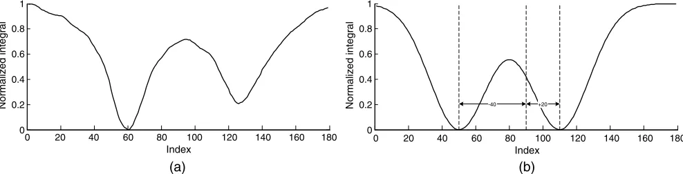
[image:4.630.327.565.551.694.2]

(5)

Figure 2(a) schematically shows our Radon transform-based feature extraction algorithm. Before using Radon transform, weights are defined for each pixel on the basis of distance from the centerline point ON. Since the closest pixels to ON have more valuable information, the corresponding weights are higher (weights close to 1). Based on a cubic interpolation, the weighted line integrals are computed and form a vector con-taining 179 elements. Figure 2(b) shows an example of the extracted features. For this example, we assume that vessels are darker than the background (for retinal images), hence it is obvious that the middle elements of the extracted vector have smaller values compared to marginal ones.

In each step, our goal is to make a prediction of the direc-tional variationtNþ1for a new input vectorxNþ1by evaluating the predictive distribution pðtNþ1jtN;x1; : : : ;xN;xNþ1Þ. Using Eq. (9), the distribution over target values is directly given by

pðtNþ1Þ ¼NðtNþ1j0;CNþ1Þ: (13)

Consequently, as mentioned in Sec.2,pðtNþ1jtNÞwill be a Gaussian distribution whose mean and covariance are given by Eqs. (7) and (8), respectively. That is

pðtNþ1jtNÞ ¼NtNþ1jmðxNþ1Þ;σ2ðxNþ1Þ: (14)

SincepðtNþ1jtNÞhas a Gaussian distribution, the most prob-able value fortNþ1is a Gaussian distribution’s meanmðxNþ1Þ. Therefore,

tNþ1¼mðxNþ1Þ (15)

and the new vessel direction (θNþ1) is calculated by

θNþ1 ¼θNþtNþ1; (16)

where θN is the vessel’s previous direction. For instance, mðxNþ1Þ ¼0means no change in the local direction (zero cur-vature), andmðxÞ≫0means high curvature (high directional variation) in a vessel.

In order to find a new centerline point, we move forward a step in the new vessel direction (θNþ1). The step length has an inverse relationship with tNþ1, i.e., when the curvature increases, the step length decreases, and vice versa. More spe-cifically, we use the following relation to obtain the step length, d, at each iteration:

d¼1 π

π

2−tNþ1

: (17)

To generate training data, shown in Figs.2(d),4(b), and5(d), synthetic images are designed to simulate vascular structure. Vessels with various curvatures and diameters and also different kinds of bifurcations are modeled for both uniformly dark ves-sels and those having reflections around their centerlines which frequently occur in retinal images, caused by light reflection from vessel surfaces that are parallel to the incident light.37

By moving along the centerline in the synthetic images and computing Radon transform, two sets of training data are gen-erated for tracking both the directional variation and diameter of the lumen. To further enrich the training data, some noise was also added to the synthetic images before computing the Radon features. Examples of these synthetic images are shown in Fig.3. Each training data has a target value corresponding to the directional variation. For instance, in Fig.2(d), the corre-sponding target value for the dotted, solid, and dashed lines

a1

a2

a90

a179

θN

0 20 40 60 80 100 120 140 160 180 0

0.2 0.4 0.6 0.8 1

Index

0 20 40 60 80 100 120 140 160 180 Index

ON

ON-1

ON+1

tN+1

tN

θN– 1

θ N

θN+ 1

-40 +40

Normalized integral

0 0.2 0.4 0.6 0.8 1

Normalized integral

(a) (b)

(c) (d)

Fig. 2 Radon features and tracking of a simple vessel: (a)aishows the result of Radon transform in each

direction. (b) A real extracted feature vector. (c) Schematic of blood centerline tracking algorithm,Oi,θi,

andtirepresent the centerline points, vessel local directions, and its variation, respectively. (d) Samples

[image:5.630.66.571.63.325.2]

(6)

are−40 deg, 0 deg, andþ40 deg, respectively, showing direc-tional variation for each one.

In summary, our vessel centerline tracking method can be explained as follows [see Fig.2(c)]. First, a seed point is selected and its corresponding feature vector is computed using the Radon transform. Then, a target directional variation is com-puted using Eq. (7). Finally, by adding this variation to the pre-vious direction, a new vessel direction is calculated. Moving a step forward along the new direction, this process continues until the end of the vessel is reached.

3.1.1 Estimation of the Kernel hyperparameter

The update process given in Eq. (16) requires evaluating a covariance matrix whose elements, in this paper, are defined using a radial basis function given by

kðxn;xmÞ ¼expð−αkxn−xmk2Þ; (18)

whereαis a hyperparameter controlling the degree of the cor-relation between the data points. We learn the latter from the training data by maximizing the likelihood function pðtNjαÞ with regard toα. In practice, we use a gradient descent approach, where we update the values ofαby moving along the gradient direction until convergence. Using the definition of a standard multivariate Gaussian distribution, the log likelihood function can be written as

EQ-TARGET;temp:intralink-;e019;326;752lnpðtjαÞ ¼− 1

2 lnjCNj− 1 2t

T_C−1

N t− N

2 lnð2πÞ: (19)

Therefore, the gradient of the log likelihood function with respect to the parameterαis calculated as

∂

∂α lnpðtjαÞ ¼−

1 2tr

C−_N1∂CN

∂α

þ1

2t T_C−1

N ∂C_N

∂α C −1

N t:

(20)

Furthermore, with respect to the predefined kernel [Eq. (18)], ∂CN

∂α elements are evaluated using

∂Cðxn;xmÞ

∂α ¼−kxn−xmk

2 _exp_ð₋_α_k_x

n−xmk2Þ

¼−kxn−xmk2kðxn;xmÞ: (21)

By following Eqs. (20) and (21), a good convergence is often achieved after 110 gradient iterations, taking less than 1 min.

3.2 Bifurcation Detection

Thus far, tracking of only simple vessels with no bifurcations was described. To obtain a more comprehensive description of the entire vascular tree, bifurcations must be detected and used to initiate further tracking. Note that, facing a bifurcation, the proposed algorithm in Sec.3.1will track the path with the smaller directional change, because it is hypothesized that cur-vature in a blood vessel has a zero mean Gaussian distribution. Therefore, using only one GP, a branch with a larger deviation angle can be dismissed. To address this problem, we will, therefore, use multiple GP’s to enable tracking through both branches.

A different set of Radon transform-based features are used to detect the branching points. As shown in Fig.4(a), in the case of a bifurcation, the obtained feature vector may indicate two local minimums that correspond to the existing branches. Therefore, in order to track both, two directions are predicted in each step. To achieve this, we use a simple approach where two indepen-dent GPs are implemented to track the smaller and larger deviation angles, respectively.

In theN’th step, lettN;1andtN;2be targets of the two inde-pendent GPs. We assume thattN;1andtN;2indicate the left and right branches, respectively, thus tN;1≤tN;2. For example in Fig. 4(b), we have tN;1¼−40 and tN;2¼ þ20. In order to train GPs, bifurcation training data should also be added to

0 20 40 60 80 100 120 140 160 180 0

0.2 0.4 0.6 0.8 1

Index

0 20 40 60 80 100 120 140 160 180 Index

-40 +20

Normalized integral

0 0.2 0.4 0.6 0.8 1

Normalized integral

(a) (b)

Fig. 4 Extracted feature in a bifurcation: (a) a real extracted feature vector. (b) A synthetic feature vector

with the corresponding target values attN;1¼−40andtN;2¼ þ20.

Fig. 3 Examples of synthetic images to generate training data are

[image:6.630.61.305.59.191.2] [image:6.630.67.561.597.723.2]

(7)

the previous data. Hence, for each training data,tN;1and tN;2, take different or the same values to represent a bifurcation or simple vessel points, respectively. For example, in Fig. 2(d)

for the doted profile, we define tN;1¼tN;2¼−40, whereas for the bifurcation shown in Fig.4(b), the corresponding targets are set astN;1¼−40and tN;2¼ þ20.

Having the training data, the kernel parameter is first estimated (see Sec. 3.1.1). Next, at each step, two Gaussian distributions, i.e., pðtNþ1;1jtN;1Þ andpðtNþ1;2jtN;2Þ are used to estimate the new target values at the means given by

tNþ1;1 ¼m1ðxNþ1Þ ¼kTC−N1tN;1; (22)

tNþ1;2 ¼m2ðxNþ1Þ ¼kTC−N1tN;2; (23)

wheretN;1andtN;2denote the left- and right-hand side branch values, respectively.

The difference between tNþ1;1 and tNþ1;2 directions is considered to be an indicator of a branching point. More specifically, if this difference becomes larger than 30 deg, we consider the current position as a bifurcation point. This thresh-old has been selected based on cross-validation experiments, minimizing the detection error on training data with known bifurcation points. Finally, when the difference between the estimated directional variations becomes less than the specified threshold, the smaller value is chosen for moving along the vessel centerline.

3.3 Diameter Estimation

In addition to the vessel centerline, diameter values are also tracked using an independent GP. Here, we assume that the diameter varies smoothly around its initial value following a nonzero mean Gaussian distribution given by

pðrNÞ ¼NðrNjr0;JNÞ; (24)

where r0 and JN represent the vessel’s initial diameter and covariance matrix, respectively.

The process of diameter tracking remains similar to before with exceptions due to some minor alterations due to the nonzero mean property of the GP. More specifically, Eq. (7) is reformulated as follows:

mðzNþ1Þ ¼aþkTJ−N1ðr−aÞ: (25)

aandzNþ1denote the mean of the GP and the feature vector in theNþ1’th step, respectively.JN and kare the kernelized covariance and similarity vector defined as earlier [see Eq. (18)]. Note that in this section, we use a different set of Radon features which are more appropriate for thickness detection. Namely, in each step after estimating vessel direction, we let

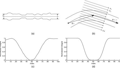
α¼θNþ1, and vary ρ to generate diameter sensitive features as shown in Fig.5(b). In this way, the line integrals are com-puted along the vessel direction, resulting in more robustness to random intensity variations across the vessel lumen. An example of such an extracted feature is shown in Fig. 5(c). A brief review of the proposed method is given in Algorithm1.

r0

θN

θN +1

b₁ b2

bM

0 10 20 30 40 50 60 70 80 90 100 Index

0 0.2 0.4 0.6 0.8 1

Normalized integral

0 0.2 0.4 0.6 0.8 1

Normalized integral

(a) (b)

(c) (d)

Fig. 5Feature extraction method for diameter estimation: (a) we assume that vessel diameter changes

smoothly along the initial diameter, (b) settingα¼θNþ1, we compute Radon transform for various values

[image:7.630.68.559.428.705.2]

(8)

4 Experimental Results

In this section, we briefly introduce the criteria that are used to quantify the performance of the proposed algorithm and review the characteristics of the data sets. Next, using various noisy images, the robustness of the methods is investigated and com-pared with other state-of-the-art techniques.

4.1 Performance Criteria

The performance is evaluated based on classification of pixels into positive (vessel) and negative (background) groups. At the final stage of the tracking step, the centerline and diameter tracking results are used to construct a binary image, segment-ing the vascular network from the background. Pixels in the neighborhood of each centerline point with radiusdare con-sidered as vessel, wheredindicates the corresponding diam-eter. By comparing the segmentation result to the reference labeled data, we are able to quantify segmentation quality. We evaluate sensitivity, specificity, and Matthew’s correlation coefficient (MCC).

Sensitivity (SN), measured by the ratio of the number of cor-rectly classified vessel pixels to the total number of vessel pixels in the image field of view [TP∕ðTPþFNÞ], reflects the ability of the algorithm to detect the vessel pixels. Specificity (SP) is the ability to detect nonvessel pixels and is measured by the ratio of

the number of correctly classified background pixels to the total number of background pixels [TN∕ðTNþFPÞ].

The MCC is often used to measure the quality of a binary classification system when the size of samples in the two classes varies substantially. In retinal fundus images, around 10% of the pixels belong to the vessels; therefore, the MCC can be used to evaluate the algorithm’s performance. The MCC is defined as

MCC¼ ffiffiffiffiffiffiffiffiffiffiffiffiffiffiffiffiffiffiffiffiffiffiffiffiffiffiffiffiffiffiffiffiffiffiffiffiffiffiffiffiffiffiffiffiffiffiffiffiffiffiTP∕N−S×P

P×_S×ð₁₋_SÞ×ð₁₋_PÞ

p ; (26)

whereN¼TPþTNþFPþFNis the total number of pixels of the image, S¼ ðTPþFNÞ∕N, and P¼ ðTPþFPÞ∕N. MCC returns a value between−1andþ1, whereþ1indicates a per-fect prediction, 0 indicates a random prediction, and−1 indi-cates a completely wrong prediction.

4.2 Databases

The DRIVE, STARE, CHASEDB1, and high-resolution fundus (HRF) databases are common databases used in this research to evaluate the performance of the proposed methods. The DRIVE database38consists of 40 color retinal images divided into train-ing and test sets, and obtained from a diabetic retinopathy screening program in The Netherlands. Each image has a size of 565×_{584 pixels} _{with eight bits per color channel.}

For the test images, two manual segmentations are available, set A and set B. 12.7% and 12.3% of pixels were marked as vessels in sets A and B, respectively. The performance is evalu-ated on the test set using set A, which is the ground truth.

The STARE database39_{consists of 20 color retinal images}

with sizes of700×_{605 pixels}_{and eight bits per color channel}

each, and are available in the PPM format. The database con-tains two sets of manual segmentations acquired by two differ-ent observers. The first observer segmdiffer-ented 10.4% of the pixels as vessels and the second one segmented 14.9%. Performance is evaluated using the first observer as the ground truth.

The CHASEDB1 dataset40_{consists of 28 color retinal fundus}

images with sizes of999×_{960 pixels}_{, acquired from both the}

left and right eyes of 14 child subjects enrolled in the program Child Heart And Health Study in England. The data set contains two groups of manually segmented images provided by two observers. The public HRF image dataset41_{contains 45 images}

with the size of3504×_{2336 pixels}_{, divided into healthy,}

glau-coma, and diabetic retinopathy groups. Ground truth segmenta-tion for these images has been made by a group of experts. For these datasets, we use green channel images as they provide a maximal contrast between vessels and the background.42

4.3 Qualitative Sample Results

The method described in Sec.3.1is able to track locally linear vessels without bifurcations. Figure6 shows results obtained from this algorithm when applied to real and synthetic data. The method is able to successfully track narrow and low con-trasted vessels as well as considerable diameter variations, sim-ulating stenoses and vasodilations in a synthetic vessel [see Fig.6(b)].

Figure7shows the performance of the same algorithm when applied to simulated and real vessels having bifurcations. As shown in Figs.7(a)and7(c), in addition to the missing branches, the bifurcation points are erroneously displaced in both cases. This error can be explained due to the use of a single GP,

Algorithm 1 Blood vessel tracking algorithm.

Input:Seed point and vessel initial diameter

Output:Vessel direction and diameter

1. Compute the vessel direction-related features using Radon transform (ρ¼0)

2. Estimate the kernel’s hyperparameter value

3. Generate the covariance matrix used to estimate the directional variation

4. Calculatet1andt2based on Eqs. (22) and (23)

5.if(t1−t2>30)then

6. {Bifurcation:}

7. Estimate new vessel directions for each branch

8.else

9. {Simple Vessel}

10. Select minimum oft1ort2as directional variation

11. Estimate new direction

12.end if

13. Compute diameter-related features using Radon transform (θ¼θNþ1)

14. Generate the covariance matrix used to estimate the vessel diameter

15. Estimate the vessel diameter (rNþ1) using Eq. (25)

(9)

which allows for tracking only one branch at a time, and the intensity information from the missing branch disturbs the proc-ess and causes deviations of the predicted centerline in the vicin-ity of the bifurcation. By using two GPs, as shown in Figs.7(b)

and 7(d), we can both resolve the localization problem and effectively detect the bifurcations.

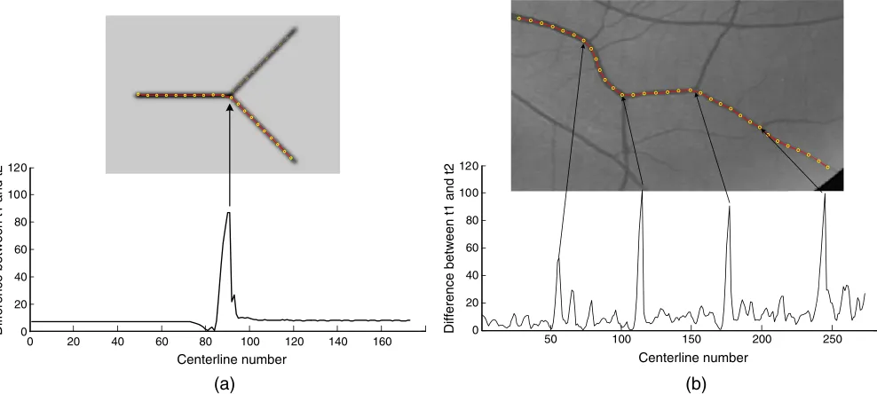
By moving forward along the vessel centerlines without bifurcations, a negligible difference betweent1andt2is detected and by approaching bifurcations, the difference increases. This is demonstrated using simulated and real images in Figs.8(a)

and8(b), respectively. As seen, the difference betweent1andt2 also shows the angle in the given bifurcation. In this paper, we apply a simple thresholding onjt1−t2jto detect bifurcations. To determine its value, we run cross validation experiments using 20 DRIVE data sets, where the threshold value is opti-mized to minimize the detection error. This process results in 30 deg as the optimal threshold. The example results in using multiple GPs for tracking narrow vessels in noisy images, and vessels with reflections on the centerlines are shown in Fig.9. It is worth noting that there are crossover points in retinal images that are required to be detected. The algorithm is able to track the main branches when two branches are perpendicular. However, approaching a crossover where the branches are not

0 20 40 60 80 100 120 140 160

Centerline number Centerline number

0 20 40 60 80 100 120

50 100 150 200 250

Difference between t1 and t2 0

20 40 60 80 100 120

Difference between t1 and t2

(a) (b)

Fig. 8 Approaching the bifurcations, the difference betweent1andt2(the predicted directional changes)

increases. Examples of (a) phantom and (b) retinal images.

Fig. 7Performance of the proposed algorithm in bifurcation. (a, c) Centerline deviation in bifurcations

using a single GP and (b, d) bifurcation detection using two independent GPs.

Fig. 6 Examples of vessel tracking and diameter estimation are

[image:9.630.64.304.59.271.2] [image:9.630.90.540.347.448.2] [image:9.630.69.563.501.723.2]

(10)

perpendicular, the algorithm behaves the same as bifurcations and tracks both branches. In the final step, for generating a binary image, the algorithm eliminates the overlapped points.

4.4 Quantitative Results

The proposed algorithm is robust against the imaging noise owing to using the Radon transform and application of GP. In this section, we quantify its robustness by segmenting a few sets of synthetic images degraded with variable degrees of Gaussian noise. The maximum and minimum levels of inten-sities in these images are set to be zero and one. For visual

examination, some of these phantom images along with the acquired segmentations are shown in Fig.10. The quantitative results are also shown in Table 1. Despite adding a strong Gaussian noise with a variance of 0.5, the algorithm segments the images with an average sensitivity of 62.81%. Furthermore, the obtained segmentation matches the target vessels to a large extent.

Table1also shows the capability of the algorithm in tracking the vessels until their end, even in the presence of excessive noise. In general, sensitivity decreases as the variance of noise increases, which can be associated with the poor accuracy in the estimated diameters. As the integration region for diameter

Fig. 10 Phantom images affected by various levels of Gaussian noise (left) used to evaluate the

robust-ness of the proposed algorithm, and their corresponding results (right). Variances in each row are (a) 0, (b) 0.05, and (c) 0.5, respectively.

Fig. 9 Sample vessel tracking and bifurcations detection in retinal images. The original images (left) and

[image:10.630.108.523.59.270.2] [image:10.630.67.565.477.716.2]

(11)

estimation is far smaller than that for direction estimation, features obtained for the former can be noisy, leading to the degraded performance, hence a reduction in the sensitivity.

4.5 Comparison with Other State-of-the-Art

Techniques

[image:11.630.324.564.84.526.2]

The proposed method has been compared to the state-of-the-art based on the values of sensitivity, specificity, and MCC mea-sures, reported in the literature. Tables2and3show the results obtained for each of the test images in the DRIVE and STARE databases, respectively. It can be noticed that the proposed

Table 1 Results obtained from segmentation of images in Fig.10by

adding different values of Gaussian noise. lin, bif, cir, and sin indicate linear, bifurcation, circle, and sinuous phantom, respectively.

Noise variance Image SN SP MCC

0 lin 0.9989 0.9999 0.9989

bif 0.9632 0.9993 0.9760

cir 0.9996 0.9962 0.9406

sin 0.9262 0.9970 0.9411

Avg 0.9720 0.9981 0.9641

0.01 lin 0.9970 0.9992 0.9880

bif 0.8979 0.9994 0.9355

cir 0.9947 0.9970 0.9642

sin 0.9097 0.9977 0.9357

Avg 0.9498 0.9983 0.9558

0.05 lin 0.9357 0.9999 0.9669

bif 0.9139 0.9997 0.9507

cir 0.9139 0.9992 0.9417

sin 0.9121 0.9970 0.9330

Avg 0.9189 0.9989 0.9481

0.1 lin 0.8224 0.9999 0.9017

bif 0.8207 0.9996 0.8972

cir 0.8372 0.9997 0.9074

sin 0.8359 0.9983 0.8965

Avg 0.8291 0.9993 0.9007

0.5 lin 0.6211 0.9999 0.7813

bif 0.6391 0.9991 0.7754

cir 0.6463 0.9995 0.7893

sin 0.6061 0.9996 0.7626

Avg 0.6281 0.9995 0.7772

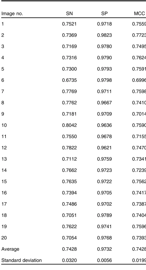
Table 2 Segmentation performance of the proposed method on the

DRIVE database.

Image no. SN SP MCC

1 0.7521 0.9718 0.7559

2 0.7369 0.9823 0.7723

3 0.7169 0.9780 0.7495

4 0.7316 0.9790 0.7624

5 0.7300 0.9793 0.7591

6 0.6735 0.9798 0.6996

7 0.7769 0.9711 0.7598

8 0.7762 0.9667 0.7410

9 0.7181 0.9709 0.7014

10 0.8042 0.9636 0.7590

11 0.7550 0.9678 0.7155

12 0.7822 0.9621 0.7470

13 0.7112 0.9759 0.7341

14 0.7662 0.9723 0.7239

15 0.7635 0.9722 0.7562

16 0.7394 0.9705 0.7417

17 0.7486 0.9702 0.7387

18 0.7051 0.9789 0.7404

19 0.7622 0.9741 0.7596

20 0.7054 0.9768 0.7393

Average 0.7428 0.9732 0.7428

[image:11.630.65.309.99.582.2]

Standard deviation 0.0320 0.0056 0.0199

Table 3 Segmentation performance of the proposed method on

the STARE database.

Image no. SN SP MCC

1 0.7100 0.9719 0.7049

2 0.7241 0.9822 0.7421

3 0.7317 0.9623 0.6134

4 0.7688 0.9807 0.7851

5 0.7046 0.9830 0.7583

6 0.6933 0.9823 0.7401

[image:11.630.325.567.575.741.2]

(12)

method reaches an average sensitivity of 74.28% and 74.19%, specificity of 97.32% and 97.06%, and MCC of 74.28% and 72.48% on the DRIVE and STARE databases, respectively. Table 4 reports the results achieved on the new published CHASEDB1 and HRF databases. Results are increased in terms of specificity. An average sensitivity of 75.35% and 77.15%, specificity of 97.67% and 97.57%, and MCC of 70.62% and 72.09% are achieved on the CHASEDB1 and HRF databases, respectively. Table4compares the performance of the proposed algorithm with other state-of-the-art techniques on the DRIVE, STARE, CHASEDB1, and HRF databases. Overall, MCC is improved on average on the CHASEDB1 dataset, when com-pared to Refs.41and 30.

The proposed algorithm is able to successfully track tiny vessels. This is due to integration of the local intensities that are used to compute the Radon transformations in conjunction with the smoothness in the centerlines made by GP. However, missing some branches due to blood vessel discontinuity, which is one disadvantage of the tracking approach, adversely affects the sensitivity of the algorithm.

[image:12.630.61.304.69.385.2]

The quantified results can be interpreted as follows: the specificity of the proposed algorithm is relatively high due to using local information around blood vessels and ignoring back-ground pixels and regions far away from the vessel centerline. However, the algorithm suffers from undesirable properties. The hypothesis for diameter estimation is that the corresponding distribution of vessel diameter is Gaussian with a mean at the initial diameter value. Considering the symmetry of Gaussian distribution, the hypothesis assumed is equivalent to equality of the diameter frequencies with smaller and larger values than

Table 3(Continued).

Image no. SN SP MCC

8 0.7104 0.9725 0.7262

9 0.7461 0.9627 0.7077

10 0.7308 0.9636 0.6930

11 0.7456 0.9718 0.7074

12 0.7700 0.9711 0.7503

13 0.7549 0.9697 0.7341

14 0.7427 0.9766 0.7453

15 0.7395 0.9725 0.7391

16 0.7490 0.9726 0.7575

17 0.7248 0.9719 0.7273

18 0.7838 0.9576 0.7182

19 0.7682 0.9545 0.6972

20 0.8067 0.9583 0.7178

Average 0.7419 0.9706 0.7248

[image:12.630.64.568.426.746.2]

Standard deviation 0.0282 0.0084 0.0348

Table 4 Comparison of the proposed algorithm with existing methods using the DRIVE, STARE, CHASEDB1, and HRF databases.

DRIVE STARE CHASEDB1 HRF

Methodology Year SN SP MCC SN SP MCC SN SP MCC SN SP MCC

Human observer — 0.7760 0.9730 0.7601 0.8951 0.9387 0.7225 0.7425 0.9793 0.7475 — — —

Martinez-Perez et al.43 ₂₀₀₇ _0.7246 _0.9655

— 0.7506 0.9569 — — — — — — —

Al-Diri et al.44 ₂₀₀₉ _0.7282 _0.9551 _— _0.7521 _0.9681 _— _— _— _— _— _— _—

Marn et al.42 ₂₀₁₁ _0.7067 _0.9801

— 0.6944 0.9819 — — — — — — —

You et al.45 ₂₀₁₁ _0.7410 _0.9751 _— _0.7260 _0.9756 _— _— _— _— _— _— _—

Miri and Mahloojifar46 ₂₀₁₁ _0.7352 _0.9795 _— _— _— _— _— _— _— _— _— _—

Odstrcilik et al.41 ₂₀₁₃ _0.7060 _0.9693

— 0.7847 0.9512 — — — — 0.7741 0.9669 —

Zhao et al.7 ₂₀₁₄ _0.7354 _0.9789 _— _0.7187 _0.9767 _— _— _— _— _— _— _—

Roychowdhury et al.47 ₂₀₁₅ _0.7390 _0.9780 _— _0.7320 _0.9840 _— _— _— _— _— _— _—

Azzopardi et al.28 ₂₀₁₅ _0.7655 _0.9704 _0.7475 _0.7716 _0.9701 _0.7335 _0.7585 _0.9587 _0.6802

— — —

Zhang et al.32 ₂₀₁₆ _0.7743 _0.9725 _— _0.7791 _0.9758 _— _0.7626 _0.9661 _— _0.7978 _0.9717 _0.7410

Strisciuglio et al.29 ₂₀₁₆ _0.7777 _0.9702 _0.7525 _0.8046 _0.9710 _0.7536 _— _— _— _— _— _—

Annunziata et al.48 ₂₀₁₆

— — — 0.7128 0.9836 — — — — 0.7128 0.9836 —

Orlando et al.30 ₂₀₁₇ _0.7897 _0.9684 _0.7556 _0.7680 _0.9738 _0.7417 _0.7277 _0.9712 _0.7046 _0.7874 _0.9584 _0.6897

(13)

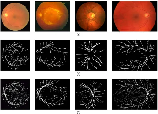
the initial diameter. However, since in retinal images vascular diameters decrease when moving away from the optic disk, the frequency of vessels with diameters smaller than the initial diameter is often greater. Thus, the diameters of narrow vessels are often overestimated as larger, lowering the specificity. This limitation happens at bifurcation and crossover points where the vessel width might not be continuous. Nevertheless, in contrary to pixel-based methods, the proposed tracking method provides direct diameter estimations and decomposes the vascular tree into constitutive branches. Sample segmentations obtained using our method are shown in Fig.11, which shows a reason-able resemblance to the reference segmentations.

The average processing time per image in DRIVE and STARE databases is about 90 s (Ubuntu 14.04 64 bit, used one processor core of Intel Core i7 @ 2.40 GHz and 8 GB RAM). It is worth noting that computational complexity for inverting a covariance matrix isOðn3_Þ_{and this fact along with the present} integration in Radon transform would lead to more computa-tional complexity compared with the other methods.

5 Discussion and Conclusion

Considering the outbreak of diabetes, its effect on retinal ves-sels, and the growing demand for periodical examination of reti-nal images, the automatic areti-nalysis of retireti-nal images is a relevant problem in medical image processing. In this paper, we

presented a new approach to track blood vessel centerlines and their diameters based on GP and Radon transform. We assumed that for a single fragment of a vessel, its curvature and diameter are GPs whose kernel parameters are optimized by maximizing the likelihood of the data.

In order to test the performance of the algorithm, the retinal images in DRIVE, STARE, CHASEDB1, and HRF databases, with ground truth pixel labels, were used. We showed that the proposed method is robust to noise and thus able to track thin structures and central arterial reflex, where the signal quality drops significantly. This property is first due to integration of the local intensities used to compute the Radon transformations. Furthermore, the smoothness in the centerlines is enforced by spatial correlations of the predictions made by GP. The result is an increased specificity level when compared to other meth-ods. The proposed method directly measures the vessel diame-ters and detects the bifurcation points that can be useful for further postquantitative and compositional analysis.

[image:13.630.63.566.57.419.2]

The proposed method relies on inverting covariance matrices and computing line integrals for Radon transformations, which can be computationally expensive. One possible interesting research direction is the development of a mechanism to make the algorithm computationally more efficient. This can be achieved using methods such as sparse GPs49,50or Fourier transforms to compute the Radon features.51,52

Fig. 11 Sample segmented results of retinal images from the DRIVE, STARE, CHASEDB1, and HRF

(14)

Disclosures

No conflicts of interest, financial or otherwise, are declared by the authors.

Acknowledgments

The authors would like to thank J. Staal,38 _{A. Hoover,}39

G. Owen,40 J. Odstrcilik,41 and their colleagues for making their databases publicly available.

References

1. X. Jiang and D. Mojon,“Adaptive local thresholding by verification-based multithreshold probing with application to vessel detection in reti-nal images,”IEEE Trans. Pattern Anal. Mach. Intell.25(1), 131–137

(2003).

2. M. D. Abràmoff, M. K. Garvin, and M. Sonka,“Retinal imaging and image analysis,”IEEE Rev. Biomed. Eng.3, 169–208 (2010).

3. H. R. Taylor and J. E. Keeffe,“World blindness: a 21st century perspec-tive,”Br. J. Ophthalmol.85(3), 261–266 (2001).

4. M. D. Abràmoff et al.,“Automated early detection of diabetic retinopa-thy,”Ophthalmology117(6), 1147–1154 (2010).

5. E. Trucco et al.,“Validating retinal fundus image analysis algorithms: issues and a proposalvalidating retinal fundus image analysis algo-rithms,”Invest. Ophthalmol. Visual Sci.54(5), 3546–3559 (2013).

6. O. Faust et al.,“Algorithms for the automated detection of diabetic reti-nopathy using digital fundus images: a review,”J. Med. Syst.36(1), 145–157 (2012).

7. Y. Q. Zhao et al.,“Retinal vessels segmentation based on level set and region growing,”Pattern Recognit.47(7), 2437–2446 (2014).

8. N. Patton et al.,“Retinal image analysis: concepts, applications and potential,”Prog. Retinal Eye Res.25(1), 99–127 (2006).

9. D. Lesage et al.,“A review of 3D vessel lumen segmentation techniques: models, features and extraction schemes,” Med. Image Anal.13(6), 819–845 (2009).

10. M. R. K. Mookiah et al.,“Computer-aided diagnosis of diabetic reti-nopathy: a review,”Comput. Biol. Med.43(12), 2136–2155 (2013). 11. M. M. Fraz et al.,“Blood vessel segmentation methodologies in retinal

images: a survey,”Comput. Meth. Programs Biomed.108(1), 407–433

(2012).

12. T. Teng, M. Lefley, and D. Claremont,“Progress towards automated diabetic ocular screening: a review of image analysis and intelligent sys-tems for diabetic retinopathy,”Med. Biol. Eng. Comput.40(1), 2–13

(2002).

13. A. F. Frangi et al.,“Multiscale vessel enhancement filtering,”inInt.

Conf. on Medical Image Computing and Computer-Assisted

Intervention, pp. 130–137, Springer (1998).

14. R. Manniesing, M. A. Viergever, and W. J. Niessen,“Vessel enhancing diffusion: a scale space representation of vessel structures,”Med. Image Anal.10(6), 815–825 (2006).

15. Y. Sun,“Automated identification of vessel contours in coronary arterio-grams by an adaptive tracking algorithm,”IEEE Trans. Med. Imaging

8(1), 78–88 (1989).

16. Y. Yin, M. Adel, and S. Bourennane,“Retinal vessel segmentation using a probabilistic tracking method,”Pattern Recognit.45(4), 1235–1244

(2012).

17. C. Kirbas and F. Quek,“A review of vessel extraction techniques and algorithms,”ACM Comput. Surv. (CSUR)36(2), 81–121 (2004).

18. S. R. Aylward and E. Bullitt,“Initialization, noise, singularities, and scale in height ridge traversal for tubular object centerline extraction,”

IEEE Trans. Med. Imaging21(2), 61–75 (2002).

19. Y. Xu et al.,“An improved algorithm for vessel centerline tracking in coronary angiograms,”Comput. Meth. Programs Biomed.88(2), 131–

143 (2007).

20. M. Tavakoli et al.,“A complementary method for automated detection of microaneurysms in fluorescein angiography fundus images to assess diabetic retinopathy,”Pattern Recognit.46(10), 2740–2753 (2013).

21. R. Pourreza et al.,“A Radon transform based approach for extraction of blood vessels in conjunctival images,” in Mexican Int. Conf. on

Artificial Intelligence (MICAI 2008), pp. 948–956, Springer (2008).

22. Q. Zhang and I. Couloigner,“Accurate centerline detection and line width estimation of thick lines using the Radon transform,” IEEE Trans. Image Process.16(2), 310–316 (2007).

23. O. Chutatape, L. Zheng, and S. Krishnan,“Retinal blood vessel detec-tion and tracking by matched Gaussian and Kalman filters,”inProc. of the 20th Annual Int. Conf. of the IEEE Engineering in Medicine and Biology Society, Vol. 6, pp. 3144–3149, IEEE (1998).

24. E. Bekkers et al.,“A multi-orientation analysis approach to retinal vessel tracking,”J. Math. Imaging Vision49(3), 583–610 (2014).

25. R. Abielmona et al.,“Vessel tracking and anomaly detection using level 0/1 and high-level information fusion techniques,”inSoft Computing

Applications, pp. 769–780, Springer (2016).

26. Y. A. Tolias and S. M. Panas, “A fuzzy vessel tracking algorithm for retinal images based on fuzzy clustering,” IEEE Trans. Med. Imaging17(2), 263–273 (1998).

27. A. Gooya et al.,“A variational method for geometric regularization of vascular segmentation in medical images,”IEEE Trans. Image Process.

17(8), 1295–1312 (2008).

28. G. Azzopardi et al.,“Trainable COSFIRE filters for vessel delineation with application to retinal images,”Med. Image Anal.19(1), 46–57 (2015).

29. N. Strisciuglio et al.,“Supervised vessel delineation in retinal fundus images with the automatic selection of B-COSFIRE filters,” Mach. Vision Appl.27(8), 1137–1149 (2016).

30. J. I. Orlando, E. Prokofyeva, and M. B. Blaschko,“A discriminatively trained fully connected conditional random field model for blood vessel segmentation in fundus images,”IEEE Trans. Biomed. Eng.64(1), 16–

27 (2017).

31. P. Liskowski and K. Krawiec,“Segmenting retinal blood vessels with deep neural networks,”IEEE Trans. Med. Imaging35(11), 2369–2380

(2016).

32. J. Zhang et al.,“Robust retinal vessel segmentation via locally adaptive derivative frames in orientation scores,” IEEE Trans. Med. Imaging

35(12), 2631–2644 (2016).

33. C. M. Bishop et al.,Pattern Recognition and Machine Learning, Vol.1, Springer, New York (2006).

34. C. E. Rasmussen,Gaussian Processes for Machine Learning, MIT Press, Cambridge, Massachusetts (2006).

35. D. J. MacKay,“Introduction to Gaussian processes,”NATO ASI Ser. F

Comput. Syst. Sci.168, 133–166 (1998).

36. L. M. Murphy,“Linear feature detection and enhancement in noisy images via the Radon transform,”Pattern Recognit. Lett.4(4), 279–

284 (1986).

37. H. Narasimha-Iyer et al.,“Automatic identification of retinal arteries and veins from dual-wavelength images using structural and functional fea-tures,”IEEE Trans. Biomed. Eng.54(8), 1427–1435 (2007).

38. J. Staal et al.,“Ridge-based vessel segmentation in color images of the retina,”IEEE Trans. Med. Imaging23(4), 501–509 (2004).

39. A. Hoover, V. Kouznetsova, and M. Goldbaum,“Locating blood vessels in retinal images by piecewise threshold probing of a matched filter response,”IEEE Trans. Med. Imaging19(3), 203–210 (2000).

40. C. G. Owen et al.,“Measuring retinal vessel tortuosity in 10-year-old children: validation of the computer-assisted image analysis of the retina (CAIAR) program,”Invest. Ophthalmol. Visual Sci.50(5), 2004–2010

(2009).

41. J. Odstrciliki et al.,“Retinal vessel segmentation by improved matched filtering: evaluation on a new high-resolution fundus image database,”

IET Image Process.7(4), 373–383 (2013).

42. D. Marn et al.,“A new supervised method for blood vessel segmentation in retinal images by using gray-level and moment invariants-based fea-tures,”IEEE Trans. Med. Imaging30(1), 146–158 (2011).

43. M. E. Martinez-Perez et al.,“Segmentation of blood vessels from red-free and fluorescein retinal images,”Med. Image Anal. 11(1), 47–61

(2007).

44. B. Al-Diri, A. Hunter, and D. Steel,“An active contour model for seg-menting and measuring retinal vessels,” IEEE Trans. Med. Imaging

28(9), 1488–1497 (2009).

45. X. You et al.,“Segmentation of retinal blood vessels using the radial projection and semi-supervised approach,”Pattern Recognit.44(10), 2314–2324 (2011).

46. M. S. Miri and A. Mahloojifar,“Retinal image analysis using curvelet transform and multistructure elements morphology by reconstruction,”

(15)

47. S. Roychowdhury, D. Koozekanani, and K. Parhi,“Iterative vessel seg-mentation of fundus images,”IEEE Trans. Biomed. Eng.62(7), 1738–

1749 (2015).

48. R. Annunziata et al.,“Leveraging multiscale hessian-based enhance-ment with a novel exudate inpainting technique for retinal vessel seg-mentation,”IEEE J. Biomed. Health Inf.20(4), 1129–1138 (2016).

49. M. Seeger, C. Williams, and N. Lawrence,“Fast forward selection to speed up sparse Gaussian process regression,”inArtificial Intelligence

and Statistics 9, no. EPFL-CONF-161318 (2003).

50. E. Snelson and Z. Ghahramani, “Sparse Gaussian processes using pseudo-inputs,” in Advances in Neural Information Processing

Systems, pp. 1257–1264 (2005).

51. G. Beylkin,“Discrete radon transform,”IEEE Trans. Acoust. Speech Signal Process.35(2), 162–172 (1987).

52. A. Averbuch et al.,“A framework for discrete integral transformations II—the 2D discrete Radon transform,”SIAM J. Sci. Comput.30(2), 785–803 (2008).

Masoud Elhami Aslreceived his BSc degree in biomedical

engineer-ing from Sahand University of Technology in 2012 and his MSc degree in biomedical engineering from Tarbiat Modares University in 2015. Subsequently, he joined R&D department of Saadat Co and worked on ECG signal analysis. Currently, he is a visiting researcher in the Norwegian Colour and Visual Computing Laboratory (ColorLab) at NTNU, Norway. His research interest includes machine learning in medical image analysis and biological signal processing.

Navid Alemi Koohbananireceived his bachelor’s degree from the

University of Isfahan in 2013 and master’s degree from Tarbiat Modares University in 2015. He is now working toward his PhD in the Department of Computer Science, University of Warwick, Coventry. His research interests are medical image analysis and machine learning.

Alejandro F. Frangi(Alex) obtained his undergraduate degree in

telecommunications engineering from the Technical University of Catalonia in Barcelona in 1996 and his PhD at the Image Sciences Institute of the University Medical Center Utrecht in 2001 on model-based cardiovascular image analysis. He is a professor of biomedical image computing at the University of Sheffield (USFD), Sheffield, United Kingdom. He leads the Center for Computational Imaging and Simulation Technologies in Biomedicine and is the academic coordinator of the MSc Bioengineering: Imaging and Sensing program.

Ali Gooyaobtained his MSc degree in electrical engineering from