White Rose Research Online URL for this paper:
http://eprints.whiterose.ac.uk/112594/
Version: Accepted Version
Article:
Das, Tushar, Simmons, David orcid.org/0000-0002-9136-6635 and Urbański, Mariusz
(2017) Dimension rigidity in conformal structures. Advances in Mathematics. pp.
1127-1186. ISSN 0001-8708
https://doi.org/10.1016/j.aim.2016.12.034
[email protected] https://eprints.whiterose.ac.uk/
Reuse
This article is distributed under the terms of the Creative Commons Attribution-NonCommercial-NoDerivs (CC BY-NC-ND) licence. This licence only allows you to download this work and share it with others as long as you credit the authors, but you can’t change the article in any way or use it commercially. More
information and the full terms of the licence here: https://creativecommons.org/licenses/
Takedown
If you consider content in White Rose Research Online to be in breach of UK law, please notify us by
arXiv:1504.01774v2 [math.DS] 29 Dec 2016
TUSHAR DAS, DAVID SIMMONS, AND MARIUSZ URBA ´NSKI
Abstract. Let Λ be the limit set of a conformal dynamical system, i.e. a Kleinian group acting on either finite- or infinite-dimensional real Hilbert space, a conformal iterated function system, or a rational function. We give an easily expressible sufficient condition, requiring that the limit set is not too much bigger than the radial limit set, for the following dichotomy: Λ is either a real-analytic manifold or a fractal in the sense of Mandelbrot (i.e. its Hausdorff dimension is strictly greater than its topological dimension).
Our primary focus is on the infinite-dimensional case. An important component of the strategy of our proof comes from the rectifiability techniques of Mayer and Urba´nski (’03), who obtained a dimension rigidity result for conformal iterated function systems (including those with infinite alphabets). In order to handle the infinite dimensional case, both for Kleinian groups and for iterated function systems, we introduce the notion of pseudorectifiability, a variant of rectifiability, and develop a theory around this notion similar to the theory of rectifiable sets.
Our approach also extends existing results in the finite-dimensional case, where it unifies the realms of Kleinian groups, conformal iterated function systems, and rational functions. For Kleinian groups, we improve on the rigidity result of Kapovich (’09) by substantially weakening its hypothesis of geometrical finiteness. Moreover, our proof, based on rectifiability, is entirely different than that of Kapovich, which depends on homological algebra.
Another advantage of our approach is that it allows us to use the “demension” of ˇStan′
ko (’69) as a substitute for topological dimension. For example, we prove that any dynamically defined version of Antoine’s necklace must have Hausdorff dimension strictly greater than 1 (i.e. the demension of Antoine’s necklace).
Contents
1. Introduction 2
2. Statement of results 5
3. Demension rigidity 8
4. A general rigidity theorem 11
5. Proof of Meta-rigidity Theorem 4.4(d <∞) 16
6. Proof of Meta-rigidity Theorem 4.4(d=∞,k= 1) 19
7. Pseudorectifiability 22
8. Proof of Meta-rigidity Theorem 4.4(d=∞,k >1) 33 9. Proof of Lemma 8.5 (Eliminating the exceptional case) 39 Appendix A. An example regarding pseudorectifiability 42
References 45
2010Mathematics Subject Classification. Primary 53C24, 20H10, 28A80, 37F35.
Key words and phrases. dimension rigidity, conformal dynamics, Hausdorff dimension, rectifiability, Kleinian groups, iterated function systems, iteration of rational functions, Julia sets.
1. Introduction
Beginning with historical perspective, our problem has roots in Poincar´e’s 1883M´emoire sur les groupes klein´eens, in which Poincar´e famously described his investigations into the surprising geometric intricacy of the “limit curves” of a certain family of discrete groups [59,§8]. These groups, generated by inversions in a simple closed chain of circles externally tangent to each other, had been presented to Poincar´e by Klein in the course of their 1881-1882 correspondence [60, p.102], and their limit sets are notable for being perhaps the first examples of “naturally occurring” fractals. For groups in this class such that the limit curve is not a circle, Poincar´e argued that at every parabolic point, the curve had a tangent line but no osculating circle.1 He went on to conjecture that no point of the limit curve which was not a parabolic limit point could have a tangent line.2Both of these facts exemplify strong senses in which the limit curve is not analytic, which were deduced from the assumption that the limit curve is not a circle. Thus they are the prototype of dynamical rigidity theorems: a dichotomy between circles and fractals.
Another historically important source of fractals was the theory of rational functions, whose Julia sets are in many ways analogous to the limit sets of Kleinian groups. In 1920, Fatou proved the following dichotomy regarding these sets [28, p.250]: if some relatively open subset of the Julia set of a rational function is a simple curve that has a tangent at every point, then the Julia set must either be a generalized circle (i.e. a geometric circle or line) or an arc of a generalized circle. Recently, the hypothesis of Fatou’s theorem was weakened as follows:
Theorem 1.1 ([26, Corollary 1 and Theorem 2]; see also [7, Theorem 2]). If a relatively open subset of the Julia set J of a rational function is contained in a smooth curve (i.e. one that that has a tangent at every point), then J is contained in a generalized circle C. Moreover, in this case either J =C,J is an arc in C, or J is homeomorphic to the Cantor set.
Again this theorem can be viewed as a dichotomy: every Julia set is either contained in a generalized circle or is not contained in any smooth curve. It is interesting to ask for a strengthening of the latter case of the dichotomy by describing other fractal properties that the Julia set (or limit set in the case of Kleinian groups) must have in that case. The first result in this direction was given in 1979 by R. Bowen [16], who showed that the limit set of a convex-cocompact quasi-Fuchsian group3is either a generalized circle or has Hausdorff dimension strictly greater than 1. Bowen’s result was improved by D. P. Sullivan [74], P. J. Braam [17], R. D. Canary and E. C. Taylor [18], and finally by C. J. Bishop and P. W. Jones, who proved the following:
Theorem 1.2 ([12, Corollary 1.8]). Let G ≤ Mob(Cb) be a finitely generated Kleinian group, and let Λ denote the limit set ofG. Then eitherΛ is totally disconnected,Λis a generalized circle, or the Hausdorff dimension ofΛ is>1.
1In modern notation, anosculating circle for a setK at a pointp ∈ Kis a circle C such that for allx∈ K,d(x, C) =
o(kx−pk2
).
2Poincar´e writes, “De plus j’ai tout lieu de croire qu’il n’y `a pas de tangente aux points deLqui ne font pas partie deP” [59,
p.79] (“Also I have every reason to believe that there are no tangent points ofLthat are not part ofP”). HereLis the limit curve andP the set of parabolic points. In the case of loxodromic fixed points, the conjecture was proven by Fricke in 1894 [31] (see also [32, pp.399-445]). Although it seems that there has been no interest in the conjecture for the last 120 years, we give the full solution below (Remark 5.6).
3A convex-cocompact Kleinian group G≤Mob(Cb) isquasi-Fuchsian if it is conjugate to some cocompact Fuchsian group
(i.e. a uniform lattice) in Mob(S1
Since Λ is compact, an equivalent way of saying that it is totally disconnected is to say that its topological dimension is equal to zero. So another way to phrase Bishop and Jones’ result is to say that if dimT(Λ)≥1,
then either Λ is a generalized circle or dimH(Λ) >1.4 This way of looking at things suggests a natural
generalization, namely that the “second case” of the dichotomy may be described by the criterion that the Hausdorff dimension is strictly greater than the topological dimension. This point of view was introduced in [48], where the following theorem was proven:
Theorem 1.3([48, Theorem 1.2]; generalized by Theorem 2.2 below). Let (ua)a∈E be a (finite or infinite,
hyperbolic) conformal iterated function system (CIFS) on Rd (3 ≤ d < ∞) which satisfies the open set condition, and let J denote the limit set of (ua)a∈E. Suppose thatdimH(J \J)<dimH(J).5 Then either
dimH(J)> k:= dimT(J), or J is contained in a generalized k-sphere.
Remark. If (ua)a∈Eis a finite parabolic CIFS (see [46] for the definition) with limit setJ, then there is an
associated infinite hyperbolic CIFS (eua)a∈Ee whose limit setJeis equal toJ minus a countable set of points
[46,§5]. So by applying Theorem 1.3 to the CIFS (eua)a∈Ee, one can see that either dimH(J)> k:= dimT(J),
orJ is contained in a generalizedk-sphere.
The proof of Theorem 1.3 uses the tools of rectifiability theory. By contrast, the following rigidity theorem due to M. Kapovich was proven using homological algebra:
Theorem 1.4 ([38, Theorem 1.3]; generalized by Theorem 2.1 below). Let G ≤ Mob(Rd) be a nonele-mentary geometrically finite Kleinian group (d < ∞), and let Λ denote the limit set of G. Then either dimH(Λ)> k := dimT(Λ), orΛ is a generalized k-sphere,6
Kapovich’s paper extended a number of earlier results. For more on the history of this result and for similar results concerning isometry groups of negatively curved spaces, see [38, p.2].
Turning back to Julia sets, the first Hausdorff dimension result was proven by D. P. Sullivan in 1982, as the result of an effort to establish a “dictionary” between Kleinian groups and rational functions [77, p.405], about which we shall say more below. Sullivan showed that if the Julia set of a hyperbolic rational map is a Jordan curve, then it is either a generalized circle or has Hausdorff dimension > 1. Sullivan’s result was improved by D. H. Hamilton, who proved the following:
Theorem 1.5 ([34, Theorem 1]). If the Julia set of a rational map is a Jordan curve, then it is either a generalized circle or has Hausdorff dimension >1.
For polynomials, the assumption that the Julia set is a Jordan curve can be weakened to merely assume that the Julia set is connected; see [78, p.168], where this is proven by combining the results of [23, 61, 82]. The parallels between Theorems 1.3-1.5 harmonize well with many other similarities between the fields of Kleinian groups, iterated function systems, and rational functions. The idea of systematically studying the analogies between the limit sets of Kleinian groups and the Julia sets of rational functions is known as Sullivan’s dictionary, since it was introduced by D. P. Sullivan [77, p.405] (see [51, 52, 74, 75, 76, 80] for
4Here and in the sequel, dim
H(S) denotes the Hausdorff dimension of a setSand dimT(S) denotes its topological dimension. The unsubscripted notation dim(S) will only be used when unambiguous, e.g. whenSis a vector space.
5An easy-to-check equivalent condition for this inequality is described in [48]. 6A subset ofRd
is called a generalized k-sphere if it is either a k-dimensional plane or a geometric sphere contained in a (k+ 1)-dimensional affine subspace ofRd
Kleinian groups and their generalizations
Conformal IFSes and GDMSes7
Rational and meromorphic functions Limit set Closure of limit set Julia set
Radial limit set Limit set Radial Julia set [66]
Poincar´e exponent Unique zero of pressure
Poincar´e exponent [62] Unique zero of pressure [64] Hyperbolic dimension [65, p.320] Dynamical dimension [65, p.320]
(these are all equal8)
Bishop–Jones theorem [12, Theorem 1]
Bowen’s formula [45, Theorem 3.15] [44, Theorem 10.2]
Bowen-type formula [6, 62, 64, 66]
Discreteness assumption Open set condition
Convex-cobounded group Finite IFS/GDMS [45, 47]
NCP map [79] with no parabolic points Special case:
Hyperbolic rational map [80, §2]
Geometrically finite group
[15] Finite parabolic IFS [46]
NCP map [80, Definition 4.1], [79] Special cases:
Parabolic rational map [80,§3] Geometrically finite rational map [53] Patterson–Sullivan measure
[56, 73]
δ-conformal measure [45, p.10]
δ-conformal measure [80, Definition 1.4], [76, Theorem 3] Patterson density of
a Gibbs cocycle [58, p.3]
Equilibrium/Gibbs state of a potential function [47,§2.2]
Equilibrium/Gibbs state of a potential function [39, 49]
Table 1. A three-way dictionary between the theories of Kleinian groups, dynamics of ra-tional functions, and conformal iterated function systems, extending Sullivan’s Dictionary, which consists of the first and last columns. We put the IFS column in the middle because in some sense the theory of IFSes “interpolates” between the theory of rational functions and the theory of Kleinian groups; for example, the fact that it extends to higher dimen-sions is shared with Kleinian groups, while in the theory of rational functions it is often useful to consider an infinitely generated IFS generated by inverse branches of iterates of a rational function.
more discussion of Sullivan’s dictionary). Sullivan’s dictionary has been the inspiration for many theorems both in the theory of Kleinian groups and the theory of rational functions, including the result of Sullivan mentioned above. In many cases, similar proofs work to demonstrate theorems on both sides of Sullivan’s dictionary.
Although the theory of iterated function systems is not traditionally considered to be part of Sullivan’s dictionary, the similarities between it and the other two fields seem significant enough that we include it as a column in our version of Sullivan’s dictionary, Table 1. Thus in our framework, Theorems 1.3-1.5 can all be regarded as variations of a more general “meta-theorem” which applies to all conformal dynamical systems. In fact, in this paper we will prove such a meta-theorem (namely Theorem 4.4) and show that it implies a sequence of theorems (namely Theorems 2.1-2.3) which are similar in spirit to Theorems 1.3-1.5.
The main purpose of this paper is not just to unify these results, but also to extend them to infinite dimensions. Such an extension can be made both in the Kleinian groups and IFS settings, although not in the rational function setting (since holomorphic maps in several complex variables are not conformal). Some motivation for studying the theory of infinite-dimensional Kleinian groups can be found in [21,§1.3]. The strategy of our proof is to extend the rectifiability argument of [48] to infinite dimensions by introducing the notion ofpseudorectifiability, a notion which agrees with the notion of rectifiability for finite-dimensional sets but not for infinite-dimensional ones. We develop the theory of pseudorectifiable sets to the extent of its applicability to our rigidity proof. As a side note, we also show that in infinite dimensions, the notions of pseudorectifiablility and rectifiability already disagree in the realm of limit sets of conformal iterated function systems satisfying the strong open set condition. It would be interesting to study the pseudorectifiability condition further, in the context of nonlinear functional analysis and geometric analysis in infinite dimensions.
Another important goal of this paper is to improve the finite-dimensional versions of these results by replacing the topological dimension with the “demension” of M. A. ˇStan′ko [72]. The demension of a
set in Euclidean space is an integer which is always at least the topological dimension of that set and is sometimes strictly greater. A standard example is Antoine’s necklace, which has demension 1 but topological dimension 0. For more on demension see §3, in which we state a theorem which implies that any “dynamically defined” version of Antoine’s necklace has Hausdorff dimension>1 (Corollary 3.6).
Acknowledgements. The authors thank R. J. Daverman and G. A. Venema for permission to re-use a figure from their book. The research of the first-named author was supported in part by a 2014-2015 Faculty Research Grant from the University of Wisconsin–La Crosse. The research of the second-named author was supported in part by the EPSRC Programme Grant EP/J018260/1. The research of the third-named author was supported in part by the NSF grant DMS-1361677. The authors thank the anonymous referee for valuable comments.
2. Statement of results
Convention 1. Throughout this paper,
• All measures and sets are assumed to be Borel.
• For eachδ≥0,Hδ denotes theδ-dimensional Hausdorff measure.
• Hdenotes a real separable Hilbert space (either finite- or infinite-dimensional). • d= dim(H)∈N∪ {∞}, and 1≤k≤dis fixed (k6=∞).
• Ifµis a measure onX andf :X →Y, thenf(µ) =µ◦f−1 denotes the image measure.
Convention 2. The symbols.×,&×, and≍×will denote coarse multiplicative asymptotics. For example, A.×,K B means that there exists a constant C >0 (the implied constant), depending only on K, such
that A≤CB. In general, dependence of the implied constant(s) on universal objects such as those given in the hypotheses of the main theorems will be omitted from the notation.
The notationA≍× B should not be confused with the notationµ≍ν, which as usual means that the
measuresµandν are equivalent, i.e. each is absolutely continuous to the other.
In the following theorems, we use somewhat unconventional notation: we useK to denote the first row of Table 1, and we useL to denote the second row. The reason for this is that if we used a more standard notation, such as Λ orLfor the first row and Λror Lr for the second row, then this notation would look
somewhat awkward when applied to the second column of Table 1: Λ orLwould denote the closure of the limit set and ΛrorLrwould denote the limit set. So instead, we use the lettersK andL, which hopefully
have less connotative baggage. (The fact thatKsuggests a compact set is a connotation we want to keep, since in the hypotheses of our theorems we assume thatKis compact.)
For definitions of the terms used in Theorems 2.1-2.3, see the proof of Lemma 4.2 below.
Theorem 2.1. LetGbe a group of M¨obius transformations ofH, and letKandLdenote the limit set and the radial limit set ofG, respectively. If d=∞, assume additionally that Kis compact. Let δ= dimH(L)
andk= dimT(K), and assume that
(2.1) Hδ(K\L) = 0
(which holds, for example, ifdimH(L)<dimH(K)). Then the following dichotomy holds: eitherδ > k, or
K is a generalized k-sphere.
Theorem 2.2. Let (ua)a∈E be a (finite or infinite, hyperbolic) conformal iterated function system on
H which satisfies the open set condition. Let L denote the limit set of (ua)a∈E, and let K denote the
closure ofL. If d=∞, assume additionally that K is compact and that (ua)a∈E satisfies the strong open
set condition. Let δ = dimH(L) and k = dimT(K), and assume that (2.1) holds. Then the following
dichotomy holds: either δ > k, or K is the closure of a relatively open and relatively compact subset of a real-analytic k-dimensional manifold M ⊆ H. If d≥3 (or more generally if (ua)a∈E consists of M¨obius
transformations), then in the latter case M is a generalized k-sphere. If (ua)a∈E consists of similarities,
then in the latter caseM is ak-plane.
Theorem 2.3. Let T :Cb→Cb be a rational function, and letK andL denote the Julia set and the radial Julia set of T, respectively. Letδ= dimH(L) andk = dimT(K), and assume that (2.1)holds. Then the
following dichotomy holds: either δ > k, or K is either a generalized circle or a segment of a generalized circle (ifk= 1) or the entire Riemann sphere (if k= 2).
Remark. Theorem 2.1 implies Theorem 1.4, which in turn implies Theorem 1.2 modulo [12, Theorem 1.2]. Theorem 2.2 implies Theorem 1.3. Theorem 2.3 doesn’t quite imply Theorem 1.5, due to the additional hypothesis (2.1), about which we will say more below.
Remark. It is worth noting that in Theorems 2.1-2.3, the weaker inequality δ≥kfollows directly from (2.1) and the classical Szpilrajn theorem:
Theorem 2.4(Szpilrajn’s theorem, [37, Theorem VII.2]). Let X be a metric space and letk= dimT(X).
Then Hk(X)>0. In particular, dim
H(X)≥dimT(X).
Letting X =K, we get Hk(K)>0. On the other hand, ifδ < k then (2.1) implies that Hk(K\L) =
Hk(L) = 0, a contradiction. So δ≥k.
Theorem 2.5 ([25, Theorem 1.8.10]). Let M be a k-dimensional topological manifold and suppose that
S⊆M satisfies dimT(S) =k. ThenS has nonempty interior relative toM.
Theorems 2.4 and 2.5 will both be used in the proof of Theorems 2.1-2.3.
Possible weakenings. We now discuss to what degree it is possible to weaken the hypotheses of Theorems 2.1-2.3.
The hypothesis (2.1). For many examples, this hypothesis is satisfied trivially, since the set K\L has Hausdorff dimension zero. In particular, this is true for geometrically finite Kleinian groups (e.g. [21, Theorem 12.4.5]), finitely generated conformal IFSes (trivially sinceK=L), topological Collet–Eckmann rational functions [63, p.139, para.3], rational functions with no recurrent critical points [79, Theorem 6.1], and certain more general classes of rational functions [67, Corollary 6.3]. However, the hypothesis cannot be removed entirely, as the following examples illustrate:
• By modifying the construction of [57], one can show that for anyε >0 and for any compact nowhere denseF ⊆ H, there exists Ga discrete group of M¨obius transformations such that dimH(L)≤ε
but K\L =G(F). By lettingF be a rectifiable set which is not a generalized sphere, one gets a counterexample to a hypothetical generalization of Theorem 2.1. A similar construction would give a counterexample to a hypothetical generalization of Theorem 2.2.
• In [5], a quasi-Fuchsian group is constructed such thatKis rectifiable but not a generalized circle, and in [10], another quasi-Fuchsian group is constructed such that dimH(K) = dimT(K) = 1 but
Kis not rectifiable.
It is an open question whether the hypothesis (2.1) can be replaced by the hypothesis that Gis finitely generated. The question is solved ford= 2 by Theorem 1.2, but higher dimensions are still open (cf. [38, Conjecture 1.4] for a related conjecture).
It is also open whether Theorem 2.3 holds if the hypothesis (2.1) is removed; cf. [9, p.207], where the same question is asked but with the assumption dimT(K) = 1 replaced by the slightly stronger assumption
thatK is connected. If this hypothesis is strengthened even further to the assumption thatKis a Jordan curve, then the question is solved by Theorem 1.5. In the other direction, if “rational function” is replaced by “transcendental meromorphic function” or “transcendental entire function”, then the answer is known to be negative [35, 11].
The open set condition and strong open set condition. The only reason that these conditions are needed in Theorem 2.2 is to ensure that Bowen’s Formula holds (cf. [45, Theorem 3.15], [44, Theorem 10.2]). So if (ua)a∈Eis an iterated function system for which Bowen’s Formula holds, then the open set hypothesis
is not necessary. For example, this holds when (ua)a∈E is chosen at random from a family of iterated
function systems satisfying the transversality condition [71]. Note that ifd=∞, then a counterexample to Bowen’s formula which satisfies the open set condition but not the strong open set condition is given in [44, Theorem 11.1].
The assumption that T is a rational function. It is natural to weaken this assumption to the hypothesis thatT :C →Cb is a meromorphic function. As it turns out, our proof is valid assuming that
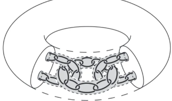
Figure 1. The first- and second-level iterates of Antoine’s necklace construction. In the IFS version of this construction, the generators for the IFS are similarities that send the large torus into the smaller tori. Since the IFS satsifies the strong separation condition, its limit setKwill be totally disconnected. On the other hand, ifγis a loop through the “hole” of the large torus, thenγis not homotopic to zero inH \K, and thusπ1(H \K)6= 0 (see e.g. [13,§2]). Figure used with permission from [22, Figure 2.5].
3. Demension rigidity
This section concerns an improvement of Theorems 2.1-2.3 (in the finite-dimensional case) in which the topological dimension is replaced by the “demension” (short for “dimension of embedding”) of M. A. ˇStan′ko
[72]. It can be skipped on a first reading, since it will not be used in the proofs of Theorem 2.1-2.3.
3.1. Demension. Our rigidity theorems 2.1-2.3 are in a sense motivated by Theorem 2.4, which shows a pre-existing relation (independent of dynamics) between the Hausdorff dimension of a set S⊆ H and its topological structure. A natural question is whether Theorem 2.4 is a complete description of the relation between Hausdorff dimension and topology. The answer is in a sense yes, and in a sense no. The sense in which the answer is yes is that any set S ⊆ H is homeomorphic to a set S′ ⊆ H such that dimH(S′) = dimT(S′) = dimT(S). This is the converse to Theorem 2.4, i.e. the other direction of
Szpilrajn’s theorem [37, Theorem VII.5]. The sense in which the answer is no is that the homeomorphism betweenSandS′ may not be extendable to all ofH.
The best way to illustrate this is with an example. Consider Antoine’s necklace construction [4] (cf. Figure 1), in which a torus in R3 is replaced by a chain of linked tori, each of which is then replaced by a smaller chain of linked tori, and so on infinitely until the intersection is a compact setS(a “necklace”) homeomorphic to the Cantor set. Ifγis a loop through the hole of the first torus, thenγis not contractible inR3\S[13,§2]. On the other hand, ifS′⊆R3is the standard Cantor set, thenR3\S′is simply connected.
Thus, the homeomorphism betweenSandS′cannot be extended to all ofR3. For this reason,Sis sometimes called a “wild” Cantor set.
Given a compact setS⊆ H, what is the smallest possible Hausdorff dimension among sets homeomorphic toSsuch that there is a homeomorphism extendible to all ofH? This question was answered by J. V¨ais¨al¨a [81]: it is thedemension of the setS:
Definition 3.1. Thedemension of a setS⊆ H, denoted dem(S), is the largest integerk such that there exists a piecewise linear polyhedronP of dimension (d−k) andε >0 such that for every continuous map
F :H ×[0,1]→ Hsatisfying the following conditions:
(II) For allt∈[0,1],
kFtk:= sup
x∈H
d(x, Ft(x))≤ε;
(III) Ft(x) =x for allx∈ H \ N(P ∩S, ε) andt∈[0,1];
we haveF1(P)∩S6=. Loosely speaking, dem(S) is the largest integer ksuch that there is a piecewise
linear polyhedronP of dimension (d−k) whose sufficiently small isotopic perturbations all intersectS.
We remark that this definition of demension is not the usual one (which is less relevant for our purposes), but is equivalent to the usual one by [24, Proposition 1.2].
Let us first address the question of how to compute the demension. The following observation is good enough to compute the demension of Antoine’s necklace and its higher-dimensional generalizations (see [13]):
Observation 3.2. IfS⊆ His a compact set such that
(3.1) π1(H \S)6= 0,
then dem(S)≥d−2.
Proof. Letγbe a piecewise linear representation of a noncontractible loop inH\S, and letP be a piecewise linear (possibly self-intersecting) 2-simplex whose boundary is γ. Fix 0 < ε < d(γ,S). Then if F is an isotopy satisfying (I)-(III), thenF1(P) is a 2-simplex whose boundary is γ. Sinceγ is noncontractible, it
follows thatF1(P)∩S6=.
In fact, a nearly complete characterization of the demension is known, but its proof requires deep topological results.
Theorem 3.3 ([24, Theorem 1.4], [69, p.598]). LetS⊆ H be a compact set. • If Sis locally homotopically 1-coconnected, thendem(S) = dimT(S).
• IfSis not locally homotopically 1-coconnected thendem(S) =d−2≥dimT(S)unless the following
case holds: d= 3,dem(S) = 2>dimT(S) = 1.
Here, the setSis said to belocally homotopically 1-coconnected if for everyx∈ Hand neighborhoodU
ofx, there exists a neighborhoodV ofxsuch that every loop inV \Sis contractible inU\S.
The “exceptional” case d = 3, dem(S) = 2 > dimT(S) = 1 can in fact occur, as demonstrated by
H. G. Bothe [14] and independently by D. R. McMillan, Jr. and W. H. Row, Jr. [50].
3.2. Demension and Hausdorff dimension. As mentioned earlier, one characterization of the demen-sion of a compact setS⊆ His that it is the infimum of the Hausdorff dimension of the image ofSunder a homeomorphism of H [81]. In particular, this implies that dimH(S) ≥dem(S). For completeness we
provide an elementary proof of a slightly stronger version of this assertion:
Theorem 3.4 ([40, Theorem 6.15]). Let S⊆ H be any set, and let k= dem(S). Then Hk(S)>0. In particular, dimH(S)≥dem(S).
Definition 3.1 such thatF1=gonU =N(P ∩S, ε/2) and kF1k< d(P \U,S\U). Sincek= dem(S), we haveF1(P)∩S6=and thusg(P)∩S6=.
LetA1, . . . , Ambe a collection of (d−k)-dimensional affine subspaces ofHsuch thatP ⊆Sm1 Ai. Then
for all sufficiently small g ∈ Isom(H), there exists i = 1, . . . , m such that g(Ai)∩S 6= . By Fubini’s
theorem, for somei= 1, . . . , mand for a positive measure set of h∈SO(H), the set ofv∈ H such that (h(Ai) +v)∩S6=is of positive measure. Equivalently,Hk(πV(h)(S))>0, whereV(h) is the orthogonal
complement of the linear part ofh(Ai) (which satisfies dim(V(h)) =k). It follows thatHk(S)>0.
Now we come to the main theorem of this section, which says that strict inequality holds in Theorem 3.4 for “dynamically defined” fractals:
Theorem 3.5. The results of§2 are still true if dimT is replaced by dem.
Corollary 3.6. For a “dynamically defined” Antoine’s necklace K (cf. Remark 3.8 below), we have dimH(K)>1.
The proof of Theorem 3.5 is given in the next section, following the statement of Theorem 4.4. The idea: where Theorems 2.4 and 2.5 are used in the proof of Theorems 2.1-2.3, instead use Theorem 3.4 and Theorem 3.7 below. Actually, the proof requires a slight strengthening of Theorem 3.4, specifically in the proof of Lemma 5.5, which is used to prove Theorem 4.4.
Theorem 3.7. Let M ⊆ H be ak-dimensional compact smooth manifold-with-boundary, and suppose that S⊆M satisfiesdem(S) =k. ThenShas nonempty interior relative toM.
Proof. Let P ⊆ H and ε > 0 be as in Definition 3.1. Without loss of generality, we can assume that P intersects M only finitely many times, and that each intersection is transversal. (This is due to the dimension relation dim(P) + dim(M) =d.) WriteP ∩M ={x1, . . . ,xm}, and without loss of generality
supposed(xi,xj)≥εfor alli6=j. Fixv1, . . . ,vm∈ Hsmall; then there exists an isotopy (Ft)t satisfying
the requirements of Definition 3.1 such that F1(x) = x+vi for all x∈ Bi := B(xi, ε/3) and such that
d(x, F1(x))≤d(P \SiBi,S\SiBi). Sincek= dem(S), we haveF1(P)∩S6=.
If v1, . . . ,vm are sufficiently small, then we can write F1(P)∩M = {g1(v1), . . . ,gm(vm)}, where
g1, . . . ,gm:U →M are smooth nonsingular maps from some neighborhood0∈U ⊆ H. So for somei, we
havegi(vi)∈S. Sincev1, . . . ,vmwere arbitrary, there existsisuch that for allv∈U, we havegi(v)∈S.
But thenScontains the relatively open setgi(U)⊆M.
Remark 3.8. It is not hard to see that in the construction of Antoine’s necklace, the small tori in the first step may be chosen to be similar copies of the large torus. (The large torus must be chosen to satisfy a certain inequality in order for this to work.) In this case, Antoine’s necklace is actually the limit set of a similarity IFS, giving a nontrivial example of Theorem 3.5. In fact, the optimality of Theorem 3.5 (for the case of necklaces) was proven by T. B. Rushing [69], who showed that for everyδ∈(1,3) there exists a similarity-generated necklace whose Hausdorff dimension isδ. (He also showed that whenδ∈ {1,3}, there exists a necklace of Hausdorff dimensionδwhich is not the limit set of a similarity IFS.)
It is interesting to ask whether the “exceptional case”d= 3, dem(S) = 2>dimT(S) = 1 can occur for
Sdynamically defined. In fact, the original construction of McMillan and Row [50] is essentially an IFS construction, although their paper does not make that very clear (which is not surprising as IFSes had not been invented yet). We hope to clarify this in future work.
4. A general rigidity theorem
In this section, we state a general rigidity theorem and show that the four theorems of the previous section all reduce to it. In this general theorem, there is no dynamical system mentioned explicitly in the hypotheses, but the hypotheses concern a measure µonHwhich should be interpreted as the conformal measure of some conformal dynamical system. To make this interpretation explicit, we include a hypothesis that a certain set Rad(µ)⊆Supp(µ) has fullµ-measure, where Supp(µ) denotes the topological support of
µ. The set Rad(µ) is supposed to represent the radial limit set of the dynamical system which generates
µ, in a way made precise by Lemma 4.2 below.
Definition 4.1. LetAbe one of the following classes:
• Conf(H), the class of conformal homeomorphisms between open subsets ofH, • Mob(H), the class of M¨obius transformations ofH,
• Sim(H), the class of similarities ofH.
Note that by Liouville’s theorem, ifd≥3 then Conf(H) = Mob(H).9Letµbe a finite measure on H, let
U ⊆ H be a bounded open set, and fix δ >0. A pointp∈Supp(µ) will be called (δ, µ)-radial (or more properly (A, U, δ, µ)-radial) if there exists a sequence of mapsgn :U → Hof classAsuch that:
(a) For all n, (1) kg′
nk:= supx∈U|gn′(x)| ≍×infx∈U|g′n(x)|;10
(2) For allx,y∈U,
kgn(y)−gn(x)k ≍×kg′nk · ky−xk;
(3) For allA⊆U,
(4.1) µ(gn(A))≥
Z
A|
g′
n|δ dµ;
(4) d(p, gn(U)).×kg′nk.
(b) kg′
nk →0.
The set of (δ, µ)-radial points is denoted Radδ(µ). Ifp∈Radδ(µ), then Cpdenotes the implied constant
of (a4) plus diam(U) times the implied constant of (a2). The significance of this is that for alln, we have
(4.2) gn(U)⊆B(p, Cpkgn′k).
Lemma 4.2. Every radial limit point of a conformal dynamical system is in Radδ(µ), where δ is the
“natural” dimension of the conformal dynamical system andµis theδ-conformal measure. More precisely, if we are in any of the following scenarios:
9The classical proof of Liouville’s theorem by Nevanlinna [55] is valid in the infinite-dimensional setting. We note in passing
that the proof in [55] is incomplete as it stands, as the fourth displayed equation on [55, p.4] is only valid under the assumption thatα6= 0: ifα= 0, then this equation should be replaced by the equationρ(x) = (v, x) +β, wherevis a constant vector andβ is a constant scalar. However, this case can be analyzed in a straightforward way, assuming that the inner product (·,·) is positive definite.
10We use the notation|g′
(1) G≤ A= Mob(H) is a group whose limit set is compact,δ is the Poincar´e exponent ofG,µis the Patterson–Sullivan measure of G, andL is the radial limit set;
(2) (ua)a∈E is a regular conformal iterated function system on H satisfying the open set condition
whose generators are of class A, δ is the Bowen parameter, µis the δ-conformal measure, and L is the limit set;
(3) H=C, T :Cb →Cb is a rational function, A= Conf(H),δ is the hyperbolic dimension, µ is the
δ-conformal measure, and Lis the radial Julia set;
then (possibly after conjugating in case (3)) there exists an open set U ⊆ H such that µ(U) > 0 and L⊆Rad(A, U, δ, µ). Moreover,
(i) in case (1), any bounded open setU for which Supp(µ)*U may be chosen; (ii) in case (2), the setU may be chosen so thatSupp(µ)⊆U.
The definitions of the terms used in this lemma will be given in the proof.
Remark 4.3. Lemma 4.2 informally says that “the radial limit set is always contained in theµ-radial set”, i.e. the inclusion L⊆Radδ(µ) always holds. On the other hand, the reverse inclusion Radδ(µ)⊆L may
fail. For example, suppose that d <∞, and letG ≤Mob(H) be a Kleinian lattice. Then µ is Lebesgue measure, and Rad(µ) =Hcontains the parabolic points ofGas well as the radial limit points ofG. This is because it is impossible to distinguish parabolic points from radial points if one only knows what µis and not what the groupGis.
Proof in case (1). LetG≤Mob(H) be a group of M¨obius transformations ofH. We recall that for each
g∈Mob(H), thePoincar´e extensionofg is the unique M¨obius transformationbg∈Mob(R⊕ H) such that
b
g ↿H=g and bg(H) =H, where H= (0,∞)× His the upper half-space model of hyperbolic space. The limit set ofGis the set
K={x∈Hb:∃gn∈G bgn(e0)→x},
wheree0= (1,0)∈H. ThePoincar´e exponent ofGis the infimum of alls≥0 such that the series
Σs(G) =
X
g∈G
e−sdH(e0,bg(e0))
converges, wheredHdenotes the hyperbolic metric onH. Since, in the assumptions of this lemma, the limit
set K is compact, there exists a Patterson–Sullivan measure µ (cf. [20, Th´eor`eme 5.4] or [21, Theorem 15.4.6]), which is a measure onK satisfying the transformation equation
(4.3) µ(g(A)) =
Z
A|
g′
|δ dµ (g
∈G, A⊆Hb).
Finally, the radial limit set L ⊆ K is the set of all p ∈ K with the following property: There exists a sequence (gn)∞1 in G such that if H : H → (0,∞) denotes projection onto the first coordinate, then
b
gn(e0)→pand
(4.4) kbgn(e0)−pk.×H(bgn(e0)) ∀n.
there exists a loxodromic isometryh∈Gwhose fixed points are both inV [21, Proposition 7.4.7], and by replacinghby a sufficiently large iterate, we can assume thatV ∪h(V) =Hb (cf. [21, Theorem 6.1.10]).
Fixp∈L, and letbgn(e0)→pbe a sequence satisfying (4.4). For eachn, choosehn∈ {id, h}such that
h−1
n g−n1(∞)∈V. It is not hard to see that ifgn is replaced by gnhn in (4.4), then the inequality remains
valid after changing the constant C appropriately. Thus, we may without loss of generality assume that
g−1
n (∞)∈V. We now proceed to demonstrate the conditions of Definition 4.1:
(a1) SinceU, V are bounded sets andd(U, V)>0, the inclusiong−1
n (∞)∈V implies that
sup
x∈Uk
x−g−1
n (∞)k ≍× inf
x∈Ukx−g
−1
n (∞)k.
Applying the formula
|gn′(x)|=H(bgn(e0))k
e0−gn−1(∞)k2
kx−gn−1(∞)k2
demonstrates that
(4.5) |gn′(x)| ≍×H(bgn(e0)) ∀x∈U.
(a2) This follows from (4.5) and the geometric mean value theorem (e.g. [21, Proposition 4.2.4] or [1, (15) on p.19]).
(a3) This follows from (4.3).
(a4) This follows from (4.5) and (4.4).
(b) This follows from (4.5) and the convergencebgn(e0)→p.
Proof in case (2). Let (ua)a∈Ebe a (hyperbolic) conformal iterated function system (CIFS) onHsatisfying
the open set condition (OSC). We recall (cf. [45, p.6-7] for the case d < ∞ and [44, p.17] for the case 3≤d≤ ∞) that this means that
1. E is a countable (finite or infinite) index set;
2. X ⊆ His a closed bounded set which is equal to the closure of its interior;
3. (Quasiconvexity) There exists Q≥1 such that for all x,y ∈X, there exists a polygonal line γ ⊆ X
connectingxandysuch that length(γ)≤Qky−xk; 4. (Cone condition) Ifd <∞, then
inf
x∈X,r∈(0,1)
λH(X∩B(x, r))
rd >0,
whereλH denotes Lebesgue measure onH;
5. V ⊆ H is an open connected bounded set such thatd(X,H \V)>0;
6. For eacha∈E,ua is a conformal homeomorphism fromV to an open subset ofV;
7. (Open set condition) For all a∈E,ua(X)⊆X, and the collection (ua(Int(X)))a∈E is disjoint;11
8. (Uniform contraction) supa∈Esup|u′a|<1, and ifE is infinite, lima∈Esup|u′a|= 0;
9. (Bounded distortion property) For all n∈N,ω∈En, andx,y∈V,
(4.6) |u′ω(x)| ≍×|u′ω(y)|,
where
uω=uω1◦ · · · ◦uωn;
For this proof, we assume in addition that the CIFS (ua)a∈E is regular (cf. [45, p.21] (d < ∞) and [44,
p.472] (3≤d≤ ∞)), i.e.
10. (Regularity) There existsδ >0 such that
(4.7) P(δ) := lim
n→∞
1
nlog X
ω∈En
ku′ωkδ= 0.
Theδwhich satisfies (4.7) is called theBowen parameter. Thelimit set of (ua)a∈E is the set L=π(EN),
whereπ:EN→X is the coding map
π(ω) = lim
n→∞uω1n(p∗).
Hereωn1 denotes the restriction ofω∈EN to{1, . . . , n}, andp∗∈X is an arbitrary point. The regularity
of the CIFS (ua)a∈E implies the existence of a δ-conformal measure µ (cf. [45, Lemma 3.13] for the case
d < ∞ and [44, Theorem 7.1] for the case 3 ≤ d ≤ ∞), which is a measure on L which satisfies the transformation equation
(4.8) µ(A) =X
a∈E
Z
u−1
a (A)
|u′a|δ dµ (a∈E, A⊆L).
Now let ε=d(X,H \V)>0 and U =N(X, ε/3), so thatK :=L ⊆U ⊆U ⊆V. Fixp∈L, and find
ω∈EN such thatp=π(ω). For eachn, let g
n=uωn
1. We now proceed to demonstrate the conditions of
Definition 4.1:
(a1) This is a restatement of (4.6).
(a2) Note that ifd≥3, then this is a consequence of the geometric mean value theorem, but ifd≤2 an additional argument is needed. Fixx,y∈U, and letγ: [0, t0]→ Hbe the length parameterization the line segment connecting gn(x) and gn(y). Let t1 be the largest element of [0, t0] such that
γ(t1)∈gn(N(X,2ε/3)). By the mean value theorem,
kgn−1◦γ(t1)−xk ≤t1 max
t∈[0,t1]|
(gn−1)′(γ(t))| ≍×t1kg′nk−1≤ kgn′k−1· kgn(y)−gn(x)k.
If t1 = t0, then we get kgn(y)−gn(x)k &× kgn′k · ky−xk. Otherwise, we have gn−1◦γ(t1) ∈
∂N(X,2ε/3), which implies kgn−1◦γ(t1)−xk ≥ ε/3 and thus kgn(y)−gn(x)k &× kgn′k &×
kg′
nk · ky−xk. So the asymptotickgn(y)−gn(x)k &× kgn′k · ky−xk holds in either case. The
proof of the other asymptotickgn(y)−gn(x)k.×kg′nk · ky−xk is similar.
(a3) This is immediate from (4.8). (a4) In fact,p∈gn(L)⊆gn(U).
(b) This is immediate from (4.6) and the uniform contraction hypothesis.
Proof in case (3). LetT :Cb→Cb be a rational function. TheJulia set ofT is the set
K=Cb\[ U ⊆Cb: (Tn↿U)∞0 is a normal family .
Thehyperbolic dimension δof T is the supremum of the Hausdorff dimensions of closed setsF ⊆Ksuch that T ↿ F is a conformal expanding repeller (cf. [65, p.320]). By [65, Theorem 12.3.11], there exists a
δ-conformal measure µ, which is a measure onK which satisfies the transformation equation
(4.9)
Z
# A∩T−1(x)dµ(x) =
Z
A|
T′|k dµ (A
Finally, let Ldenote theradial Julia set ofT, i.e. the set of points p∈Cb such that there existε >0 and a sequencenj → ∞with the following properties (cf. [66, Definition 2.5]):
(I) For eachj, there existsφj :Bs(Tnj(p), ε)→Cb, an inverse branch ofTnj, such thatφj(Tnj(p)) =p.
Here the notationBs means that the ball is taken with respect to the spherical metric. (II) diam(φj(Bs(Tnj(p), ε)))→0.
Now fixp∈L, and letε >0 be as above. By extracting a subsequence from (nj)∞1 , we may without loss of generality suppose that Tnj(p)→q∈K. By conjugating if necessary, we can assume ∞∈/ K and in
particularq6=∞. LetU be a bounded open set containingqsuch thatU ⊆Bs(q, ε/2), and for eachj let
gj =φj ↿U. We now proceed to demonstrate the conditions of Definition 4.1:
(a1) This is a consequence of the K¨oebe distortion theorem [19, Theorem 1.4]. (a2) This is proven in the same manner as for case (2).
(a3) This is immediate from (4.9).
(a4) In fact,p∈gj(U) for all sufficiently largej.
(b) This is immediate from (a1) and part (II) of the definition of the radial Julia set.
We are now ready to state our general rigidity theorem, and prove that it implies the results of§2-3:
Theorem 4.4. Let Hbe a separable Hilbert space, and let µ be a finite measure on Hwhose topological supportSis compact. Letk= dimT(S)ork= dem(S), and suppose thatHk-a.e. point ofSis(A, U, k, µ
)-radial, where A is as in Definition 4.1 andU ⊆ H is a bounded open set such that µ(U)>0. Ifd=∞, we additionally assume thatdimT(S∩U) =k. Also suppose thatRadk(µ)is dense inS. Then there exists
a map h:U → Hof class Asuch thath(S∩U)is contained in ak-plane.
Proof of the results of §2 and of Theorem 3.5 assuming Theorem 4.4. LetA, δ,µ, andL be as in Lemma 4.2. In the case of CIFSes, this requires some justification, since the CIFS (ua)a∈E is not assumed to be
regular in Theorem 2.2, and regularity is necessary to ensure the existence of a δ-conformal measure µ. This justification comes from [45, Theorem 4.16] in the cased <∞, and from [44, Proposition 9.2] in the case 3≤d≤ ∞, since by Theorem 2.4 (or Theorem 3.4 if k= dem(K))Hk(K)>0, and by hypothesis dimH(K) =k. Thus by Lemma 4.2, we getL⊆Radδ(µ) after making an appropriate choice forU.
We claim thatδ= dimH(L). Indeed, this has been proven for Kleinian groups in [21, Theorem 1.2.1],
for CIFSes in [45, Theorem 3.15] (d <∞) and [44, Theorem 10.2] (3≤d≤ ∞ and strong OSC), and for rational functions in [66, Theorem 1.1] (see also [53, Theorem 2.1]).
Now by Theorem 2.4 (or Theorem 3.4 ifk= dem(K)) we haveδ≥k, and ifδ > k then we are done, so suppose thatδ=k. ThenL⊆Radk(µ). Since Theorems 2.1-2.3 all include the hypothesisHδ(K\L) = 0,
we getHk(K\Radk(µ)) = 0. Moreover, it is obvious thatK=S= Supp(µ).
If d = ∞, then we additionally need to verify dimT(K∩U) = k. In the case of CIFSes this follows
from (ii) of Lemma 4.2. In the case of Kleinian groups, it follows from the sum theorem for topological dimension [25, Theorem 1.5.3] that there exists a closed set F $ K such that dimT(F) = k, so we get
dimT(K∩U) =kfor allU ⊇F.
So by Theorem 4.4, there exists a map h : U → H of class A such that h(K∩U) is contained in a
k-plane. In particular,K∩U is contained in:
• ak-plane ifA= Sim(H).
We complete the proof by breaking into cases:
• To prove Theorem 2.1, let (Un)∞1 be an increasing sequence of open sets such thatK*Unfor all
nbutK\ {p} ⊆SnUn for somep∈K(andUn ⊇F ifd=∞). For eachn, by part (i) of Lemma
4.2, there exists a generalizedk-sphereSn which containsK∩Un. Since the setS=SNTn≥NSn
is the increasing union of generalized spheres of dimension≤k, it is also a generalized sphere of dimension≤k. ButK\ {p} ⊆S, and so sinceK is perfect,K⊆S.
By Theorem 2.5 (or Theorem 3.7 ifk= dem(K)),K has nonempty interior relative toS. But then the boundary ofKrelative toAis a closedG-invariant set which does not containK, hence it is empty. ThusK=S.
• To prove Theorem 2.2, let U be as in (ii) of Lemma 4.2. Then K = K∩U ⊆ M for some real-analytick-dimensional manifoldM.
By Theorem 2.5 (or Theorem 3.7 ifk= dem(K)),K has nonempty interior relative toM. Let
I be the interior ofKrelative toM. ThenI is invariant under (ua)a∈E and is therefore dense in
K. SoI is a relatively open relatively compact subset ofM whose closure is equal toK.
• To prove Theorem 2.3, we divide into cases. If k= 1, then the conclusion follows from Theorem 1.1. Ifk= 2, then by Theorem 2.5, K has nonempty interior. But then the boundary of K is a closedT-invariant set which does not containK, hence it is empty. ThusK=Cb.
The proof of Theorem 4.4 will occupy the remainder of this paper. We divide it into three cases:
d <∞; d=∞ andk = 1;d=∞and k >1. We refer to these cases as Theorem 4.4(d < ∞), Theorem 4.4(d=∞,k= 1), and Theorem 4.4(d <∞,k >1), respectively, and we prove them in Sections 5, 6, and 8, respectively. Section 7 contains preliminaries needed for the proof of Theorem 4.4(d=∞,k >1), and Section 9 contains the proof of a technical lemma needed in the proof of Theorem 4.4(d=∞,k >1).
5. Proof of Meta-rigidity Theorem 4.4(d <∞)
The basic structure of the proof may be summarized as follows:
Step 1: Show that we can without loss of generality assumeµ=Hk ↿S. In particular, this implies that Hk(S)<∞.
Step 2: Use the rigidity assumption k = dimT(S) or k = dem(S) to prove that µ-a.e. point has an
approximate tangentk-plane (Definition 5.4 below), using results from geometric measure theory. This is in some sense the key step, and generalizing it appropriately to infinite dimensions will be one of the main themes in the proof of Theorem 4.4(d=∞).
Step 3: Choose a radial limit point p∈Radk(µ) which has an approximate tangentk-plane. Then use a
“zooming argument” to finish the proof.
We remark that Step 1 does not depend on finite-dimensionality and in fact the result of this step will be used in the proof of Theorem 4.4(d=∞).
In the sequel we will often refer to the following well-known fact:
Fact 5.1. LetX andY be metric spaces, and letf :X→Y be aK-Lipschitz function, i.e. a function for which
Then for allA⊆X, Z
Y
#(f−1(x)
∩A) dHk(x)≤KkHk(A). In particular, iff is 1-Lipschitz then Hk(f(A))≤Hk(A) for allA⊆X.
Step 1: Without loss of generality, µ=Hk↿S. In this step, we will prove that: (i) ν:=Hk ↿
Sis finite and absolutely continuous to µ;
(ii) Radk(µ)⊆Radk(ν);
(iii) Supp(ν) =S= Supp(µ).
From these three facts, it follows that if we can prove Theorem 4.4 in the caseµ=ν, then it holds in the general case as well. We remark that in fact, for the applications of Theorem 4.4 used in§2, it is possible to prove thatµ=αν for someα >0 using an ergodicity argument. But for a cleaner formulation and for additional generality, we did not include an ergodicity-type hypothesis in Theorem 4.4.
The main tool for this step is the Rogers–Taylor density theorem, which in some circumstances allows one to estimate the Hausdorff measure of a set from the upper density function
Dδµ(x) = lim sup
rց0
1
rδµ(B(x, r))
of a finite measure µ. Rogers and Taylor originally proved their result for finite-dimensional Euclidean spaces [68], but it has subsequently been extended to arbitrary metric spaces.
Theorem 5.2(Rogers–Taylor density theorem, [44, Theorem 8.2], [30,§2.10.19]). LetX be a metric space, letµbe a measure on X, and fixδ >0. Then for allA⊆X,
µ(A) inf
x∈A
1
Dδµ(x)
.×Hδ(A).× µ(X) sup
x∈A
1
Dδµ(x)
·
In particular, ifDδµ is bounded from below on a setA⊆X, thenH δ↿A≤Cµfor some constantC >0. If
Dδµ is strictly positive on A, thenHδ ↿A isσ-finite and absolutely continuous to µ.
In our setting we takeX=H,δ=k, and
A= Radk(C, µ) :={p∈Radk(µ) : the implied constants in Definition 4.1 are all< C},
whereC >0 is fixed. Fixp∈A, and let (gn)∞1 be as in Definition 4.1. Then for all n, 1
(Cpkg′nk)k
µ B(p, Cpkg′nk)
≥ (C 1
pkgn′k)k
µ(gn(U))&×,C
1 kg′
nkkk
g′
nkkµ(U) =µ(U)>0.
SoDkµ(p)>0, and thus by Theorem 5.2,
(5.1) ν ↿Radk(C,µ)is finite and absolutely continuous to µ.
LetG be the collection of mapsg:U → Hof classAsuch that for allA⊆U, (4.1) holds.
Claim 5.3. Ifµ(A)>0 for someA⊆U, thenν(S\G(A)) = 0, where
G(A) = [
g∈G
Proof. Letγ=µ↿G(A). Fixp∈Radk(µ), and let (gn)∞1 be as in Definition 4.1. Then for all n, 1
(Cpkg′nk)k
γ B(p, Cpkg′nk)
≥(C 1
pkgn′k)k
µ(gn(A))&×,pµ(A)>0.
SoDkµ(p)>0, and thus by Theorem 5.2,ν =Hk↿Radk(µ) isσ-finite and absolutely continuous to γ. So
sinceγ(S\G(A)) = 0, we haveν(S\G(A)) = 0.
LetA=U in Claim 5.3. Sinceµ(U)>0 by hypothesis, we get ν(S\G(U)) = 0. On the other hand, by Theorem 2.4 (or Theorem 3.4 ifk= dem(K)),ν(S)>0, soν(G(U))>0, and so by Fact 5.1ν(U)>0. We now demonstrate (i)-(iii):
(i) Since by assumptionν(S\Radk(µ)) = 0, we haveν(Radk(µ)∩U)>0, so for someC >0, we have
ν(Radk(C, µ)∩U)>0. In particular, by (5.1),µ(Radk(C, µ)∩U)>0. LettingA= Radk(C, µ)∩U
in Claim 5.3, we get ν(S\G(Radk(C, µ)∩U)) = 0. But since the elements ofG are conformal, it follows that Radk(C, µ) is G-invariant in the sense that G(Radk(C, µ)∩U) ⊆Radk(C, µ). So
ν(S\Radk(C, µ)) = 0. Using (5.1) again, we see thatν is finite and absolutely continuous toµ.
(ii) Suppose thatp∈Radk(µ), and let (gn)∞1 be as in Definition 4.1. Fixnand letA=gn−1(H\S)⊆U.
Sinceµ(gn(A)) = 0, (4.1) shows thatµ(A) = 0, i.e. A∩S=. It follows thatgn(S∩U)⊆S, and
then Fact 5.1 and (a2) yield that (4.1) holds with µreplaced byν. Sincenwas arbitrary, we get p∈Radk(ν).
(iii) Sinceν(U)>0, it is obvious that Radk(ν)⊆Supp(ν), so this follows from (ii) together with the
hypothesis that Radk(µ) is dense inS.
Step 2: Existence of approximate tangent planes. Let us recall the definition of an approximate tangent plane:
Definition 5.4 (Cf. [43, Definition 15.17]). LetSbe a subset ofH, and letp∈Ssatisfy
lim sup
rց0
1
rkH
k S
∩B(p, r)>0.
Ak-dimensional linear subspaceL0≤ His called anapproximate tangentk-plane forSatpif for allε >0,
(5.2) lim
rց0
1
rkH
k S
∩B(p, r)\(p+Nproj(L0, ε))
= 0.
HereNproj(L0, ε) denotes the projective ε-thickening
Nproj(L0, ε) ={x∈ H:d(x, L0)≤εkxk}.
The existence of approximate tangent planes for a large measure set of points on suitably non-fractal12 subsets ofHis a combination of some well-known geometric measure theory results:
Lemma 5.5 (Non-fractality implies approximate tangent planes). Suppose thatd <∞, and let S⊆ H be a set such thatHk(S)<∞, where eitherk= dim
T(S)ork= dem(S). Then the set of points inSwhich
have an approximate tangentk-plane has positive Hk measure.
Proof. The hypothesis implies that Hk(πV(S)) > 0 for a positive measure set of k-dimensional linear subspacesV ≤ H, whereπV denotes orthogonal projection ontoV: ifk= dimT(S), then this follows from
12Here we use Mandelbrot’s terminology [41, p.38], in which a setSis called a fractal if and only if dim
[29, §9], and if k = dem(S), then this follows from the proof of Theorem 3.4. Thus by the Besicovitch– Federer projection theorem (Theorem 7.13 below), S is not purely k-unrectifiable (cf. Definition 7.11 below). The conclusion now follows from [43, Corollary 15.20].
Since in our context we get either k = dimT(S) or k= dem(S) by hypothesis, and the σ-finiteness of
Hk↿Swas proven in Step 1, we get that the set of points inSwhich have an approximate tangentk-plane
has positive Hk measure. In particular, there exists a point p ∈ Radk(µ) which has an approximate
tangentk-plane.
Step 3: Zooming argument. Letpbe as above. LetL0≤ H be an approximate tangentk-plane for Satp, and let (gn)∞1 be as in Definition 4.1. Then for allε >0, by (5.2) we have
1 kg′
nkk
µB(p, Cpkgn′k)\(p+Nproj(L0, ε))
−→n 0.
Now by (a3),
µ U\g−n1 p+Nproj(L0, ε)
.×
1 kg′
nkk
µ gn(U)\(p+Nproj(L0, ε))
−→n 0.
After extracting a subsequence along which this convergence is geometrically fast, we get µ(U \Sε) = 0
and thusS∩U ⊆Sε, where
Sε=
[
N∈N
\
n≥N
gn−1 p+Nproj(L0, ε)
.
Now writeTn(x) =p+kgn′kxandhn=Tn−1◦gn∈ A; then
Sε=
[
N∈N
\
n≥N
h−n1 Nproj(L0, ε).
But by (a1), |h′
n(x)| ≍× 1 for all x∈U, and by (4.2),hn(U)⊆B(0, Cp) for alln. In particular, by the
Arzela–Ascoli theorem, (hn)∞1 is a normal family. After extracting a subsequence, lethbe the limit. Then
Sε⊆h−1 Nproj(L0, ε)
,
S∩U ⊆ \
ε>0
Sε⊆h−1
\
ε>0
Nproj(L0, ε)
!
=h−1(L0).
Since the classAis closed under normal limits, we haveh∈ A, which completes the proof.
Remark 5.6. By slightly modifying the above argument, one can show: If µ is a finite measure onH, S= Supp(µ), andU ⊆ H is an open set, then eitherS∩U is contained in a k-dimensional real-analytic manifold, or else no point of Radδ(µ) can have a tangent k-plane for S. Here a k-dimensional linear
subspace L0 ≤ H is called a tangent k-plane for S at p if for all ε > 0 there exists r > 0 such that S∩B(p, r)⊆p+Nproj(L0, ε). In particular, this proves Poincar´e’s conjecture [59, Section VIII] mentioned in the introduction, corresponding to the special case whereSis the limit set of a certain Kleinian group.
6. Proof of Meta-rigidity Theorem 4.4(d=∞,k= 1)
An analysis of the argument in Section 5 shows that the finite-dimensionality assumption was only used in two places:
2. in the use of the Arzela–Ascoli theorem in Step 3.
It turns out that when k = 1, we can find “patches” for these arguments which work in infinite di-mensions, keeping the overall proof structure of Theorem 4.4 the same. But whenk >1, a different proof structure will be needed. However, a substantial portion of this section (namely Theorem 6.3 and Corollary 6.5) will also be used in the proof of Theorem 4.4(d=∞, k >1).
We begin with a lemma which is the analogue of the first two-thirds of the proof of Lemma 5.5:
Lemma 6.1. Let S⊆ H be a compact set such that H1(S)<∞ anddimT(S) = 1. Then S contains a rectifiable curve.
Proof. Since Sis a compact set with dimT(S) = 1, there exists a connected component C ⊆S with at
least two points [25, Theorem 1.4.5]. By [70, Lemmas 3.5 and 3.7],Cis equal to a rectifiable curve.
Remark 6.2. This lemma is the only place in this section where the assumptionk= 1 is used in a crucial manner. (This fact will be important in the proof of Theorem 4.4(d=∞,k >1).) It is not clear whether the analogue of Lemma 6.1 fork >1 holds or not.
Next, we would like to say that every rectifiable curve contains approximate tangent planes, but the problem is that the usual version of the Lebesgue differentiation theorem does not hold in infinite dimen-sions. Instead, we need a variant of this theorem, which we state and prove below. When we apply this theorem to the problem of finding approximate tangent planes to rectifiable curves, it turns out that we need to replace the limit (5.2) with the limit taken along a certain sequencern ց0. The points that we
get do not necessarily have “approximate tangent planes” in the sense of Definition 5.4, but they are good enough to make the argument of Step 3 work.
Theorem 6.3 (Lebesgue differentiation theorem for general metric spaces). Let X and Y be separable metric spaces, let ν be a locally finite measure on X, and letf :X →Y be a bounded function. For ν-a.e.
p∈X, if (Bn)∞1 is a sequence of sets such that (I) diam(Bn)→0,
(II) p∈Bn for alln, and
(III) ν(4Bn)≍×ν(Bn)for alln, where
4B:=N(B,1.5 diam(B)),
then
(6.1) lim
n→∞
1
ν(Bn)
Z
Bn
dY f(p), f(x)dν(x) = 0.
Proof. This theorem follows from [30,§§2.8-2.9] but we write out the proof for clarity. For eachδ, C >0, letAδ be a countable partition ofY such that diam(A)≤δfor allA∈ Aδ, and let
CC,δ=
(
B∩f−1(A) : B⊆X, ν(4B)≤Cν(B), A∈ Aδ,
ν(B\f−1(A))
≥δν(B)
)
XC,δ=
n
x∈X : inf{diam(E) :x∈E∈ CC,δ}= 0
o .
Proof. Fixδ >0. LetA∈ Aδ be the element which containsf(p). Sincep /∈XC,δ, for all sufficiently large
nwe haveBn∩f−1(A)∈ C/ C,δ, so
ν(Bn\f−1(A))< δν(Bn).
In particular
Z
Bn
dY f(p), f(x)
dν(x)≤
Z
Bn∩f−1(A)
dY f(p), f(x)
dν(x) +
Z
Bn\f−1(A)
dY f(p), f(x)
dν(x)
≤δν(Bn) + diamY(f(X))ν(Bn\f−1(A))≤δ 1 + diamY(f(X))
ν(Bn).
Taking the limit asn→ ∞gives
lim sup
n→∞
1
ν(Bn)
Z
Bn
dY f(p), f(x)dν(x)≤δ 1 + diamY(f(X)),
and lettingδ→0 finishes the proof. ⊳
So to complete the proof, it suffices to show thatν(XC,δ) = 0 for allδ, C >0.
By contradiction, suppose that ν(XC,δ) >0 for some δ, C > 0. Then there exists A ∈ Aδ such that
ν(XC,δ∩f−1(A))>0, and by the inner regularity of ν, there exists a compact setK ⊆ XC,δ∩f−1(A)
such thatν(K)>0. LetU ⊇Kbe an arbitrary open set. Then by the definition ofXC,δ,
CC,δ,A(U) :={B⊆U :ν(4B)≤Cν(B), B∩f−1(A)∈ CC,δ}
is a cover ofK. So by the 4r-covering lemma (e.g. [44, Theorem 8.1]), there exists a disjoint subcollection D ⊆ CC,δ,A(U) such that{4B:B ∈ D}is a cover ofK. But then
ν(K)≤ X
B∈D
ν(4B)≍×,C
X
B∈D
ν(B).×,δ
X
B∈D
ν(B\f−1(A))≤ν(U\f−1(A))≤ν(U\K).
SinceU was arbitrary andν(K)>0, this contradicts the outer regularity ofν.
Applying Theorem 6.3 to our circumstance, we get:
Corollary 6.5. LetX =Sandν=µ=Hk↿
Sbe as in Theorem 4.4, and letY andf be as in Theorem
6.3. Forµ-a.e. p∈Radk(µ), if(gn)∞1 is as in Definition 4.1, then
(6.2) lim
n→∞
1 kg′
nkk
Z
gn(U)
dY f(p), f(x)dµ(x) = 0.
Proof. Letp∈Radk(µ) be a point for which
(6.3) Dkµ(p) = lim sup
rց0
1
rkµ(B(p, r))<∞;
by Theorem 5.2, (6.3) holds for µ-a.e. p∈ Radk(µ). Let (gn)∞1 be as in Definition 4.1, and let Bn =
B(p, Cpkg′nk). Then µ(4Bn).×,pkgn′kk by (6.3), butµ(Bn)≥µ(gn(U))&×,pkgn′kk by (4.2) and (4.1).
By (b) of Definition 4.1, diam(Bn)≤2Cpkg′nk →0, and by constructionp∈Bn for alln. So by Theorem
6.3, (6.1) holds for the sequence (Bn)∞1 (assumingpis not in theµ-nullset where Theorem 6.3 fails). Since
µ(Bn)≍×,pkg′nkk, (4.1) finishes the proof.
We can now prove an analogue of Lemma 5.5:
Lemma 6.6. Let S and µ = Hk ↿S be as in Theorem 4.4, with k = 1. Then there exists a positive
k-dimensional linear subspace L0≤ H such that for all ε >0,
(6.4) lim
n→∞
1 kg′
nkk
µgn(U)\(p+Nproj(L0, ε))
= 0.
Proof. By Lemma 6.1, S contains a rectifiable curve C. We recall that this means that there exists a Lipschitz surjection γ : [0,1] → C. By the infinite-dimensional version of Rademacher’s theorem [3, Theorem 3.5],γis differentiable Lebesgue-a.e. LetNbe the set of points whereγis either not differentiable or has a zero derivative. By the metric change-of-variables formula [3, Theorem 5.1],H1(γ(N)) = 0.
Let f : C → [0,1] be a measurable partial inverse ofγ, so that γ◦f(x) = x for allx ∈ C. Extend
f to Sby setting f ≡2 on S\C. Let p ∈ C∩Radk(µ)\γ(N) be a point satisfying the conclusion of
Corollary 6.5; we claim thatp satisfies the conclusion of the lemma. Let (gn)∞1 be as in Definition 4.1. Sincep∈C\γ(N),γis differentiable att:=f(p) andγ′(t)
6
=0. LetL0=Rγ′(t). Fixε >0, and letδ >0 be small enough so that for alls∈[t−δ, t+δ],
kγ(s)−γ(t)−γ′(t)(s−t)k ≤σkγ′(t)k · |s−t|,
whereε= 1−σσ. Then
γ([t−δ, t+δ])⊆p+Nproj(L0, ε).
But by (6.2),
lim
n→∞
1 kg′
nkk
µ x∈gn(U) :f(x)∈/[t−δ, t+δ] = 0,
which implies (6.4).
Armed with this lemma, no changes are needed for Step 3 of Section 5 until the last paragraph. Instead of using the Arzela-Ascoli theorem, we use Liouville’s theorem to extend hn to a M¨obius tansformation
acting on all ofHb, and then we use the fact that|h′
n| ≍×1 onU to deduce that h−n1 p+Nproj(L0, ε)∩U ⊆ N(h−n1(L0), Cε)
for some large constant C > 0. So for every n ∈ N, there exists a generalized 1-sphere Sn such that S∩U ⊆ N(Sn,2−n). From this it is not hard to see that S∩U is contained in a generalized 1-sphere,
since if the sequence (Sn)∞1 does not converge, thenS∩U will be contained in a point. (A more detailed version of this argument is given in Step 5 of the proof of Theorem 4.4(d=∞,k >1) below.)
7. Pseudorectifiability
We now begin the preliminaries to the proof of infinite-dimensional rigidity, i.e. Theorem 4.4(d=∞,
k >1).
7.1. Definition and basic properties of pseudorectifiability. Our main tool in the proof of Theorem 4.4(d=∞,k >1) will be an analogue of Lemma 5.5 based on the notion ofpseudorectifiability, a gener-alization of rectifiability. Thus, we begin by recalling the definition of rectifiability, and then introducing the definition of pseudorectifiability:
Definition 7.1. A setR⊆ His called(k-)rectifiable if there exists a countable family of Lipschitz maps fi: [0,1]k→ Hsuch that
Hk R\
∞ [
i=1
fi([0,1]k)
!