GEOFFREY A. LATHAM B. E. , B. Sc . ( Ho n s ) ( Q1d )
A t h e s i s s u b m i t t e d i n p a r t i a l f u l f i l m e n t o f t h e r e q u i r e m e n t s o f t h e d e g r e e o f
Ma s t e r o f S c i e n c e i n
Syst ems E n g i n e e r i n g a t
The A u s t r a l i a n N a t i o n a l U n i v e r s i t y Au g u s t 1984.
and has not been s ubmi t t e d f o r a hi g he r de gr e e at any o t he r
U n i v e r s i t y or I n s t i t u t i o n .
I wish t o thank P r o f e s s o r s Brian D.O. Anderson and John B. Moore f o r t h e i r i n v a l u a b l e guidance and s u p e r v i s i o n in t he p r e p a r a t i o n o f t h i s t h e s i s . Also d e s e r v i n g o f t hanks a r e Dr Bob Bitmead f o r r e a d i n g an e a r l y d r a f t and Dr Keith Glover f o r d i r e c t i n g my study o f t h e
Th is t h e s i s a d d r e s s e s the p r o b l e m of mo d el r e d u c t i o n
for s c a l a r l i n e a r t i m e - i n v a r i a n t s y s t e m s via the use of
the o p t i m a l H a n k e l - n o r m a p p r o x i m a t i o n p r o b l e m . F r e q u e n c y
w e i g h t i n g is c o m b i n e d w i t h o p t i m a l i t y in the H a n k e l n o r m
to o b t a i n a f r e q u e n c y s h a p e d a p p r o x i m a t i o n to a g i v e n
l i n e a r s y s t e m . Th is is a c c o m p l i s h e d by the s o l u t i o n of a
m o d i f i e d o p t i m a l H a n k e l - n o r m a p p r o x i m a t i o n p r o b l e m .
A b s tra c t CHAPTER 1
§1.1 In tr o d u c tio n 1
§1.2 Review 2
§1.3 Approach and C o n trib u tio n o f the Thesis 4
§1.4 Some P re lim in a ry Theorems 6
§1.5 s-numbers and the Adamjan, Arov and Krein Theorem 9
§1.6 Systems w ith a Rational A ll-p a s s Factor 13
CHAPTER 2
§2.1 I n tr o d u c tio n 17
§2.2 Discrete-Tim e Frequency Weighted Approximation 18
§2.3 L°° Errors o f the Approximation 21
§2.4 The Continuous-Time Case 23
§2.5 An Example 24
CHAPTER 3
§3.1 In tr o d u c tio n 32
§3.2 Known L -norm Bounds00 32
§3.3 E rro r Analysis 34
§3.4 Conclusion 40
CHAPTER 4
§4.1 Synopsis 42
§4.2 Future Research 42
APPENDIX
§A. 1 In tr o d u c tio n 45
§ A. 2 Continuous-Time Theory 45
CHAPTER 1
§1.1 INTRODUCTION
The approxi mat i on o f high o r d e r l i n e a r system t r a n s f e r f u n c t i o n s pl ays an i mpor t ant p a r t in many a r e a s of e l e c t r i c a l e n g i n e e r i n g . The d e s i r a b i l i t y o f r e p l a c i n g a high o r d e r model by one o f reduced o r d e r i s mot i vat ed p r i m a r i l y by t h e advant ages o f i mpl ement i ng, e i t h e r i n hardware or s o f t w a r e , as s i mpl e a system as p o s s i b l e whi l e s t i l l meet i ng t he
desi gn s p e c i f i c a t i o n s . To det er mi ne whet her an a ppr oxi mat i on scheme s a t i s f i e s any desi gn r e q u i r e me n t , t he s i z e o f t he e r r o r i n c u r r e d in making t he appr oxi mat i on shoul d be e x p l i c i t l y known, whi l e si mpl e a l g o r i t h ms f o r de t e r mi ni ng t h e appr oxi mat i on would a l s o be o f d i s t i n c t advant age.
I t i s p r e c i s e l y t h e s e f e a t u r e s t h a t have l e d t o t he keen i n v e s t i g a t i o n and a p p l i c a t i o n o f t he so c a l l e d opt i mal Hankel-norm appr oxi mat i on problem [3, 14, 27 , 36] t o model r e d u c t i o n of e n g i n e e r i n g syst ems. This t e c h n i q u e , e s s e n t i a l l y an a p p l i c a t i o n from t h e t h e o r y of Hankel o p e r a t o r s , has l e d , t o g e t h e r with t he t he or y o f b a l anc e d r e a l i z a t i o n s , t o a renewed
i n t e r e s t in model r e d u c t i o n in r e c e n t y e a r s . In p a r t i c u l a r , optimal Hankel-norm appr oxi mat i on has found wide a p p l i c a t i o n among t he f o l l o wi n g :
( i ) t he r e d u c t i o n o f high o r d e r p l a n t models t o al l ow t he desi gn of low o r d e r c o n t r o l l e r s [ 1 6 ] ,
( i i ) t he r e d u c t i o n of high o r d e r c o n t r o l l e r s desi gned us i ng t he f u l l o r d e r p l a n t model [ 27- 29] ,
( i i i ) t he r e d u c t i o n of f i l t e r d e s i g n s ,
Besides having a computationally cheap closed form solution and
calculable error bounds in terms of the frequency response, the method
gives an approximation which, as the name suggests, is optimal in a
specific measure (the Hankel-norm) and so is the f i r s t model reduction
technique to obey any strong optimality criterion. More importantly
however, is that the resulting approximation is guaranteed to be realizable.
The object of this thesis is to show how to combine the additional
feature of specifying the approximation accuracy with frequency, thereby
shaping the error of the optimal Hankel-norm approximation. This is
highly desirable since in many practical situations, i t is possible to
identify frequency regions where any approximating system should be
particularly 'close' to the original system.
For example such a region
is represented by the unity gain crossover for a closed-loop control
system. From an engineering viewpoint, the synthesis of optimal Hankel-
norm approximation and specification of error size with frequency,
combines the power of frequency domain and state space methods.
It
allows the incorporation of intuitive classical design ideas, which
provide unmatched insight and insensitivity to small errors in a system
description, with formal tractable mathematics. Like state-space methods,
the frequency-weighted approximation scheme also extends easily to
multivariable systems.
§1.2 REVIEW
The modern theory of Hankel operators has i t s beginnings in the
algebraic theory of Hankel and Toeplitz matrices and forms which
originated in the memoirs of G. Frobenius [11,12], who studied them in
connection with problems of s t a b i l i t y theory and related questions of
In the f i r s t half of this century, the study of Hankel operators gained
an important impetus from applications in function theory, probability
theory and the problem of moments [35]; however the present intense
interest in the theory can largely be attributed to the discovery of new
applications for recent advances, chiefly in function theory, Gaussian
processes and systems theory.
Important recent results include the works of Nehari [31], Hartman
[18], Adamjan, Arov and Krein [1-4], Clark [7,8] and Peller and
Khrushchev [32,33]. A complete overview of this work appears in Power
[34] and Peller and Khrushchev [33], while the progress enjoyed by the
algebraic theory is detailed in Iohvidov [20].
From the systems theoretic point of view, the most significant of
this work applicable to model reduction is that of Adamjan, Arov and
Krein [3] which appeared in English in 1971. This work went largely
unnoticed (by systems theorists) until 1978 when P. Dewilde [23] pointed
out i ts importance to the larger system theoretic community.
In
particular [3] is the source of the theory behind the optimal Hankel-
norm approximation technique which has found so many fruitful engineering
applications.
Using the theory of balanced realizations, Silverman and Bettayeb
[36] made the existence results of [3] concrete and gave explicit
algorithms for obtaining the optimal Hankel-norm approximation of any
specified order to a given finite-dimensional scalar system.
Kung and
Lin [26] employed a polynomial approach that led to a simple generalised
eigenvalue formulation of the optimal Hankel-norm problem and gave a
fast matrix-fraction description algorithm for i t s solution. This
approach was extended in [27] to obtain efficient algorithms for multi-
variable systems while [28] uses a state-space approach to solve the
A different approach is that of Harshavardhana et a l . [19] who
with the implementation of one algorithm obtained solutions of all
orders to the optimal Hankel-norm problem for a scalar system from the
eigenvectors of a bilinear matrix combination of rearranged versions of
the Hurwitz matrix for the characteristic polynomial of the system.
An interesting application to model reduction is that of Jonckheere
and Helton [22], where the order of a stochastic process power spectrum
is reduced by finding the optimal Hankel-norm approximant of the phase
of the outer spectral factor. The most complete treatment, known to
the author, of the optimal Hankel-norm approximation problem for multi-
variable systems is that of Glover [14].
[14] uses results in balanced
realizations, all-pass functions and the inertia of matrices to obtain
all solutions by solving Lyapunov equations and for one class of
solutions gives explicit error bounds in the supremum norm.
§1.3 APPROACH AND CONTRIBUTION OF THE THESIS
Underlying the work of this thesis is the considerable theory of
Hankel operators and their applications to linear systems.
From this
large body of theory, §§1.4 and 1.5 assemble some well known results,
including the main result of Adamjan, Arov and Krein about which the
thesis is developed.
§1.5 also introduces and defines an important set
of input-output invariants of a linear system; the singular values, in a
more general setting. Also presented there, is a new derivation of a
weak bound on the f i r s t singular value of the optimal Hankel-norm
approximant.
In §1.6, we derive some sh if t inequalities for the singular
values of rational functions that contain an all-pass factor.
In
particular, we partially extend a result of Glover [14], concerning the
optimal Hankel-norm approximation of stable rational all-pass systems
The work in Chapter 2 introduces and develops the central new
idea of the thesis; combining frequency weighting and optimal Hankel-
norm approximation. The basic idea involved is as follows: consider a
series combination of two stable systems the second of which is to be
approximated by a lower order system. We desire the approximation error
to be determined by the magnitude of the frequency response of the f i r s t
system. Available from the Adamjan Arov and Krein theory, is a procedure
for obtaining the explicit form of an optimal approximating system
(of reduced order) which we wish to u t i l i s e . The synthesis is performed
thus: f i r s t devise a transformation that, when applied to the f i r s t ,
frequency weighting system, produces a completely unstable system with
the same magnitude (with frequency), as the frequency weighting. Next,
combine i t with the second system to form a modified system. Apply now
the optimal Hankel-norm approximation technique to the modified system-
The modification is now "undone" by multiplying the resulting approximation
by the image of the frequency weighting under the inverse of the original
transformation.
Finally, take the stable part of the result as the
frequency-weighted optimal Hankel-norm approximation. This method is
formally developed in §§2.1 to 2.4. We conclude the chapter with a
practical example of the technique. A classical Butterworth f i l t e r is
reduced in order by two, the approximation being frequency shaped by a
simple second order system.
The core of the third chapter consists of a more thorough error
analysis of the frequency weighted optimal Hankel-norm approximation
theory presented in Chapter 2. Error bonds are derived for the incurred
error in both the supremum (L°°) and Hankel-norms so that frequency
weighting may be compared with other candidate model reduction schemes.
In particular, the bounds allow an easy comparison with those for direct
The final chapter of the thesis presents a retrospective overview,
followed by several suggestions for future research into the many new
ideas that arose during the investigations of the thesis.
The appendix is supplemental to Chapter 2 in that i t presents in
part the same theory contained in that chapter but derived independently
in continuous time with the use of integral operators.
In summary, the contribution of the thesis is f i r s t , to propose
and develop the theory of a new method for combining the optimal Hankel-
norm approximation technique with the analytical specification of the
approximation accuracy with frequency, and secondly to present an error
analysis and demonstrate the applicability of the method via a common
example from circuit theory.
§1.4 SOME PRELIMINARY THEOREMS
As a preliminary, we assemble several important known results for
Hankel operators on a Hilbert space. They will be used repeatedly in
the sequel.
Let £2 denote the Hilbert space of two-way square summable complex
sequences w = {... w2, w1} w{, w2, . . . } and £2 the (sub) Hilbert space
of one sided square summable complex sequences y = {y^, y2, . . . } . £2
CO
is endowed with the inner product (v,w) = Z (v.w. + v^vT), where the bar
j _ 1 J J J J
denotes the complex conjugate.
Let {e^, e2, . . . } denote the standard
orthonormal basis on £2.
Each operator Y on £2 has a representing matrix
Y-. = (Ye", e") with respect to the standard basis. The quantity IIYll
1J 1 J
will denote the induced operator norm on £2. The mapping determined by
oo
f (e19) = Z (f-e~1JÖ + f-e 1'
Ö) is a Hilbert space isomorphism from
j=l J
J
£2 to L2, the space of complex valued functions defined on the unit circle
"1 0Each sequence in £ 2 under the mapping y(z ) = Z determines a j = l J
member o f the Hardy class H 2, a n a ly tic in the open u n it disk. This is also a H ilb e r t space isomorphism.
oo
By L denote the space o f a l l complex valued fu n c tio n s , f , on the u n i t c i r c l e with bounded L°°-norm, ie || f || = ess s u p |f( e l w )|< 00 ,
0
OO
and H the space o f complex valued functions which are a n a ly tic and bounded in the open u n it d is k , | z | < l . I t can be seen th a t L°° C, L2 and H°°C H2. We now define a Hankel operator on £2.
D e fin it io n 1.1 A Hankel operator r on £2 is an operator fo r which there e x is ts a sequence a i , a2 , . . . such th a t i \ • = -j,
i , j = 1,2, . . .
The fo llo w in g r e s u lt allows us to con stru ct bounded Hankel operators.
Theorem 1.1 (Nehari [31 ]) The i n f i n i t e Hankel m atrix ( ai + j _ l ) ) 7 j_ i determines a bounded lin e a r operator r on £2
i f and only i f there e x is ts an L°° fun ction f such th a t an = f , where f is the n-th negative Fourier c o e f f ic ie n t o f f . That i s ,
f n = n = 1, 2, . . . . Moreover, given an f E L°°, and i f V is the Hankel operator w ith m a trix elements
r i j = ( f i + j - i ) ' i , j = i » then
II
r ll
=llf+hIL»
h G H°°> and there is a unique h ' E H°° such th a t || T \ \ = || f+ h ^ L .We w i l l c a ll f the symbol fu n c tio n o f the bonded Hankel operator r and denote the operator and m a trix , (terms which are used interchangeably),
by r ( f ) . I t w i l l sometimes be convenient to omit the symbol function
when no ambiguity can a ris e . C le a rly f o r any given bounded Hankel opera tor, the symbol fu n ctio n is not unique because r ( f ) = r(f+h) fo r a l l h E H°°. Given an f E L°°, the unique symbol fun ction f + h ' fo r
which I r ( f ) II = II f + h X > h' e h” , is c a lle d the Nehari extension o f
D e fi n it io n 1.2 Given an f G L°°, the Hankel-norm of f is defined by, || f ||H = || r ( f ) || .
Next is a characterization of the compact Hankel operators.
Theorem 1.2 (Hartman [1 8 ]). The Hankel operator r ( f ) is compact i f and only i f f e H°° + C, where C denotes the space of continuous functions on the u n i t c i r c l e .
F i n a l l y , we characterise the f i n i t e rank Hankel operators.
Theorem 1.3 (Kronecker [13,25]). The i n f i n i t e Hankel matrix
T - - = (aq-+j _ i )”
j_i
is of f i n i t e rank n, i f and only i fr(z) = is a rat ion al function of z and
z z2 z 3
th a t in t h i s case, n is the number o f poles of r ( z ) , counted with mul t i p i i c i t y .
Throughout the th e si s , we w i l l be p r im a r i l y concerned with Hankel matrices whose symbols are real rat ion al functions that represent
disc re te- time system t r a n s f e r functions. Theorem 1.1 then ensures that i f , as we w i l l assume throughout, the symbol functions have no poles on IzI = 1 , the Hankel operators w i l l be bounded. Theorem 1.2 guarantees the existence o f bounded s i n g u l a r values (see §1.5) and Theorem 1.3 implies th a t the Hankel matrices w i l l be o f f i n i t e rank
equal to the number o f stable poles (counting m u l t i p l i c i t y ) o f the symbol function. A pole or zero w i l l be cal le d stable i f i t l i e s in
I z I < 1 and unstable i f i t l i e s in |z|> 1.
oo . _
by
[ g ], = £ g^zJ"
and
[g] = g-[g]
. The projection [• ]
se l e c t s
j=l J
“
the stable part of g and projects L2 onto L2ÖH2 .
I f f G L°° define
the Hankel operator
r ( f )on H2
by
r ( f ) h = [ f h] _ = [[f]_h
]_ ,h G H2 .
This definition, which is equivalent to Definition 1.1, often
leads to simplified proofs involving Hankel and Toeplitz operators [33].
1.5 s-NUMBERS AND THE ADAMJAN, AROV AND KREIN THEOREM
An important se t of parameters of a linear system, are i t s singular
values which are the s-numbers of the associated Hankel operator.
We
now define these.
Definition 1.3
The (k+ l) -st s-number of the Hankel operator
T ( f ) , denoted
0|<+-|(f)
is defined by
Gk+l(f )
=inf
II r ( f ) - L|| k =
0,1,
2. . .
(5.1)
where the infemum is taken over all bounded linear operators
L
of rank £ k .
It can be shown [17] that
a
( f ) is the ( k + l) -st eigenvalue of
— T — V >
( T ( f ) r ( f ) ) 2 and that the s-numbers therefore form a decreasing sequence
for increasing k .
Note that according to Definition 1.2,
|| f ||H = Oi(f)
Definition 1.4
Let
a
be an s-number of
r ( f ) .A pair
(£,
n ),
n G£2 is called a Schmidt pair of
r ( f )corresponding
to
a
i f
r ( f ) £=
on
( 5. 2)and
T(f)n= oE,
D e f i n it io n 1.5 A function 0 ( z ) , not necessarily stable, is called all-pass i f <j>(z)<j>(z) = 1 f o r a l l |z| = 1 .
Important in determining the s-numbers o f a given function are the Blaschke products. A rat ion al all-pass function of the form
n .
B(z) = n e j z-aj f o r some complex numbers ai . . . a„ and where j = ! l - ä j z
a . = arg a. , is called a Blaschke product with n zeros. Note th a t the
J J ^ . __
function B(z) = B(z"- 1 ) s a t i s f i e s BB = 1 f o r a l l z and has zeros at the poles of B(z) and poles at the zeros of B(z).
The d e f i n i t i o n (5.1) may be regarded as an approximation measure that gives the smallest at ta ina ble distance from r ( f ) using rank k operators. An important con tri bu ti on o f Adamjan, Arov and Krein is the proof th a t the infemum in (5.1) is attained by a unique i n f i n i t e Hankel matrix o f rank k. In a d d it io n , t h e i r con structive proof gave a unique symbol function with exa ctly k stable poles t h a t is a distance
ak+l ( f ) ^rom ^ 1'n ^ " norm* This symbol function is called the k-th order optimal Hankel-norm approximation to f . We stat e t h e i r r e s u l t in the followin g theorem.
Theorem 1.4 (Adamjan, Arov and Krein [ 3 ] ) . Given an f G L°°, there ex is ts a unique i n f i n i t e Hankel matrix T(x) o f f i n i t e rank
k < rank r ( f ) such tha t
|| r ( f ) - r( x ) || = cr
k+i
( f ).
(5.3)Further, i f (£,n) is any Schmidt p a i r o f r ( f ) corresponding to ak +] ( f ) , then the symbol function x(z) th a t is given by
x(z) = f ( z ) - Qk+1( f ) ^ ( z ] r <5' 4)
n_(z) A 00 = 2 n,-z
i = l 1 C+(z)
= T. g.z
i = l 1 i-1 where
is the unique function th a t at t a in s the infemum in the expression
Dk( f ) = i n f I f - g L , (5.6)
9
the infemum in (5.6) being taken over a l l functions g of the form r + h where r i s a s t r i c t l y proper rat ion al function with
00
no more than k stable poles and h <= H . That is
II f - x L = Dk( f ) (5.7)
and x(z) has exactly k stable poles (counted with m u l t i p l i c i t y ) . Moreover, the functions ri_( z)/£+(z) have u n i t modulus on the u n i t c i r c l e ( i e they are a l l - p a s s ) .
A more concise proof o f t h i s theorem than that which appeared in the o r ig i n a l paper, may be found in [33] or [34]. When applying Theorem 1.4 to approximate system t r a n s f e r fun ctions, f ( z ) is a stable real rational fun ctio n. In t h i s case, i t can be shown [36] th a t the rat ion al all -p ass function q_/£+(z) has in general n+k stable poles and n-k-1 unstable poles where n is the number o f poles o f f ( z ) . Therefore to avoid re ta i n i n g unstable poles in the approximation x, [x]_ is taken as the approximating system to f ( z ) . The e q ua li ty (5.3) then holds since r ( x) = T([x]_) but o f course (5.7) is no longer v a l i d . [x]_ w i l l be called the stable k-th order optimal Hankel-norm approximation to f (z ) and x(z) w i l l be said to solve the optimal Hankel-norm approximation problem o f order k.
Lemma 1.5 [ 6 , 7 ] The s-number a^+i ( f ) may be expressed as:
a k+1( f ) = i n f || T(f) - A || (5.8)
K 1 A
= i n f || T(uf) || (5.9)
u
= i n f || f + v L (5.10)
v
where the infema are respectively taken over, Hankel operators A of rank k,
Blaschke products u with k zeros in |z |< l and ratio na l functions v with k stable poles.
Proof. S ta rt in g with ( 5 . 9 ) , we get by using Nehari's theorem (Theorem 1.1) and Kronecker's theorem (Theorem 1.3),
i n f || T(uf) || = i n f i n f || uf + h L h £ H°°
u u h
= i n f i n f || f + üh L u h
= i n f i n f || f + r + g L ; g G H°°, r regular rat ion al
r g
with k stable poles = i n f || r ( f ) - r ( r ) ||
r
= i n f || r ( f ) - A|| = a. , ( f ) .
A K 1
The l a s t eq ua li ty follows from Theorem 1.4.
The e q u a l i ti e s (5.8) and (5.10) show th a t the symbol function x of (5.4) s a t i s f i e s
II f - x l l = ok+1( f ) (5.11)
and tha t therefore ( f ) = ak+-|( f).
The e x p l i c i t form (5.4) gives the fo ll o w in g easy bound f o r
II
x||H=
Ol (x)Lemma 1.6 a i ( x ) is bounded according to
° i ( f ) - ^ k+-| ( * a i ( x ) £ o i ( f ) + a k+1( f ) . (5.12)
Proof Although (5.12) i s a t r i v i a l consequence of the equality ( 5 . 3 ) , we give a s l i g h t l y more i n s t r u c t i v e proof of the upper bound. Denote ak+^ ( f ) by o. According to ( 5 . 4 ) , on
z = en t , - tt £ t < 7T, we have | x | 2 = | f | - 2 | f | aco s(e(el t ) - arg f ( e n t )) + a2, where 0(e^^) = arg n_/C+- Thus ( | f | - o ) 2 £ | x | 2 < ( | f | + a ) 2
so t h a t I II T_1|L " Gl < II XL c II f | L + a - Because r( x ) = r(x+h) oo
f o r a l l h G H , we can replace f in Theorem 1.4 by i t s Nehari A
extension f^ and consider x = f^ - ori_/C+ • But f^ is by uniqueness j u s t the function o i ( f ) n i - / £ i + where (Ci, m ) is any Schmidt
A p a i r corresponding to O i ( f ) . The above argument then gives fo r x, ( a i ( f ) - a ) 2 <
I
x12 < ( a i ( f ) + a ) 2 . C le ar ly , Gi ( x) =a i ( x) < || x L so t h a t the upper bound immediately follows.
§1.6 SYSTEMS WITH A RATIONAL ALL-PASS FACTOR
o f such symbols. In p a r t i c u l a r , we p a r t i a l l y extend a r e s u l t i n Glover [14] on the s i n g u l a r values o f r a t i o n a l a l l - p a s s systems.
Let F(z) e L be a s t a b l e r a t i o n a l f u n c t i o n o f degree n and <j>(z) a r a t i o n a l a l l - p a s s f u n c t i o n w i t h mi s t a b l e poles and m2 unstable
poles. That i s ,
4>(z) = BiBz (6.1)
where Bi and B2 are (modulo a f a c t o r e^a , a r e a l ) Blaschke products o f
orders mi and m2 r e s p e c t i v e l y . Assume also t h a t m2 does not exceed
n-1 and t h a t no pol e- ze ro c a n c e l l a t i o n s occur in the combination F<f>. Noting t h a t a..(F) = 0 f o r i > n, we have the f o l l o w i n g Lemma.
Lemma 1 .7. For F and <j> as defi ned above,
^ ° k < F*> > < W F) k = 1 .... n-m2 (6.2)
° k + m T F<^ * V F> k = 1 .,.. n . (6.3)
Proof Using the c h a r a c t e r i z a t i o n ( 5 . 1 8 ) , we have t h a t
o k (F4>) = i n f II F<j> + u L , k = 1 . . . n+mi , where u i s r a t i o n a l u
and has < k-1 s t a b l e poles. 4 i s a l l - p a s s so t h a t a ^ ( Fcf) =
i n f II F + ? u L . According to ( 6 . 1 ) , f = BiET2 has m2 s t a b l e poles u
and 4>u has £ k-l +m2 s t a b l e poles so t h a t a^(FcJ>) > i n f || F + v L = v
o k+m2( F ) , k = 1 . . . n-m2 , where v i s r a t i o n a l and has k-l+m2 s t a b l e poles. The i n e q u a l i t y ( 6 . 2 ) i s t r i v i a l f o r k > n - m2 . S i m i l a r l y , a ^ F ) = i n f ||F. 1 + u 11^ = i n f ||FcM + u L = i n f ||Ff + <|>uL >
u u u
i n f II F<J> + v L = G|^+ ( F4>) , where v has £ k+m^ -1 s t a b l e poles.
We note i n passing the f o l l o w i n g speci al cases o f Lemma 1.7.
C o r o l l a r y 1.8 ( i ) I f B2 = 1, i e m2 = 0 and <j) t h e r e f o r e has on ly unstable zer os, then o^Fc})) > F ) , k = 1 . . . n
( i i ) I f B1 = 1, i e mi = 0 and t h e r e f o r e has o n ly
Combining ( i ) and ( i i ) o f Lemma 1.7 gives bounds on a r e s t r ic t e d set of the s in g u la r values o f F<J> as fo llo w s :
°k<F*> * a k-m l(F) m l < k £ mx +
°k<F« < < W F) 1 < k £ n - m2 so th a t when n > m 1 + m2 ,
a k+m2(F) s a k(F<l>) Ä a k-m i(F) m‘ < k < n - m2.
Glover [14] has noted the fo llo w in g r e s u lt f o r stable a ll-p a s s systems.
Lemma 1.9 Let 4>(z) be a real ra tio n a l stable a ll-p a s s function with n zeros. Then
a.jU ) = 1 i = 1 . . . n . (6.5)
Lemma 1.9 implies th a t a l l optimal Hankel-norm approximants o f a stable a ll-p a s s system are e q u id is ta n t in the Hankel-norm from the
o r ig in a l system and th a t t h i s distance is equal to 1. I t would therefore appear useless to approximate a ll-p a s s systems because the re s u ltin g e r r o r is the same size ( in Hankel-norm) as the o r ig in a l system.
Although Lemma 1.9 takes care o f stable a ll-p a s s systems, i t is not immediately c le a r th a t optimal Hankel-norm approximation o f unstable a ll-p a s s systems w i l l be successful, since Nehari's theorem im plies only th a t the s in g u la r values w i l l be * 1. Some o f the sin g u la r values
may the re fo re be s u ita b ly small. The fo llo w in g r e s u lt shows th a t certa in approximants o f unstable a ll-p a s s systems are again e q u id is ta n t from the o r ig in a l system.
o •(<!>) = 1
j = 1 . . . n-m
J ( 6. 6)
ö
.(<J>) < 1
j = n-m+1 . . . n
J
Proof <j) may be written as in (6.1) where Bi has m zeros and B2
has n > m zeros.
By Nehari's theorem,
< I <ML = 1
j = 1 . . . n .
(6.7)
According to (5.10) we also have
g
.U ) = inf || BiBl + u [ = i n f || Bl + B7
> o.
(Bi) ,
J
u
u
J
j = 1 . . . n-m .
(6.8)
By Lemma 1.9,
ö^BT) = 1
i = 1 . . . n .
Thus for j = 1 . . . n-m
(6.8) and (6.7) give (6.6 ).
Remark.
Lemma 1.10 implies t h a t all optimal Hankel-norm approximants
of order k such t h a t k £ n-m-1 will be a distance 1 from 4> in the
Hankel-norm.
Fi nally, we s t a t e the important special case j = 1 of Lemma 1.10 separately.
Corol 1 ary 1.11
I f <}>(z) is a real ratio nal a l l - p a s s function
with more st a b le than unstable poles, then
CHAPTER 2
§2.1 INTRODUCTION
T h is c h a p te r p re s e n ts a method o f fre q u e n c y shaping the e r r o r o b ta in e d by p e rfo rm in g an o p tim a l Hankel-norm a p p ro x im a tio n o f a s c a l a r , f i n i t e - d i m e n s i o n a l , l i n e a r , t i m e - i n v a r i a n t system. As was seen i n
Theorem 1 . 4 , th e o p tim a l Hankel-norm a p p ro x im a tio n procedure f i n d s a t r a n s f e r f u n c t i o n ( o r t r a n s f e r f u n c t i o n m a t r i x ) o f p r e s c r ib e d o r d e r which a p p ro xim ate s a give n t r a n s f e r f u n c t i o n ( o r t r a n s f e r f u n c t i o n m a t r i x ) o f g r e a t e r o r d e r .
One m o t i v a t io n f o r fre q u e n c y w e ig h ti n g comes from the d e s i r e to implement a reduced o r d e r a p p ro x im a tin g c o n t r o l l e r w i t h i n a c lo s e d - lo o p c o n t r o l system. Suppose an LQG designed s e r ie s compensator i s t o be used i n a c o n t r o l system im p le m e n ta tio n . The compensator w i l l have th e same dimension as th e p l a n t model. For s i m p l i c i t y , i t i s d e s i r a b l e to app ro xim a te the compensator by one o f the lo w e s t o r d e r p o s s i b l e w h il e m a in t a i n in g an o v e r a l l a c c e p ta b le d e g ra d a tio n i n perform an ce. The
a p p ro x im a tin g compensator s h o u ld be o b ta in e d in a way t h a t ta k e s accou nt o f th e fre q u e n c y c h a r a c t e r i s t i c s o f th e p l a n t model. For example i n the p l a n t stop band and a t fre q u e n c ie s o f h igh lo o p g a i n , th e d e t a i l e d
shape o f the a p p ro x im a tin g compensator i s n o t so i m p o r t a n t , however around th e u n i t y gain c r o s s o v e r fre q u e n c y , i t i s d e s i r a b l e to secure a c c u ra te a p p ro x im a tio n .
We show here how t o m o d ify the a p p ro x im a tio n method o r i g i n a l l y
developed by Adamjan, Arov and K re in [ 3 ] to a l lo w f o r fre q u e n c y w e ig h t i n g . The means f o r i n t r o d u c i n g fre q u e n c y w e ig h tin g w h il e p r e s e r v in g the
§2.2 DISCRETE-TIME FREQUENCY WEIGHTED APPROXIMATION
We f i r s t establish some preliminary notation and results.
Definition 2.1
Let G(z) be a s t r i c t l y minimum phase, s t r i c t l y
stable, real rational scalar transfer function, ie G(z) has no
poles or zeros in | z| >l, save for a possible zero at z = °°.
Let r > 0 be the smallest integer such that lim zr G(z) is nonzero.
Z-*»
Then define the "tilde" operation by
G(z) - z~r G(z_1) .
(2.1)
It may be noted here that G and G-1 are analytic in the closed unit disc.
Given a rational transfer function with Laurent expansion
CO
K(z) = ^ £ ki z ' 1
(2.2)
i = -oo
which converges in some open region containing the unit circle, |z| = 1,
then the Hankel operator r(K) = r([K]_)has matrix elements
T(K(z))ij = ki+j _1
i , j = 1,2, . . .
(2.3)
where [K]_, the stable part of K(z), is equal to the sum of those terms
in the partial fraction expansion of K(z) that have poles in |z|<l .
The tilde operation (2.1) has the desirable property of preserving
the rank of the Hankel matrix T(K) under the change K
KG. This
property is crucial and is proved in the following lemma.
Lemma 2.1
Let F(z) be a s t r i c t l y stable proper rational transfer
function and l et G(z) satisfy the conditions of Definition 2.1 and
OO
have Laurent expansion G(z) = Z 9-jz_1 >
9r / 0 , which converges
i = r
( i ) rank F(F(z)) = rank r(F(z)G(z)) (2.4) and
( i i ) r(FG) = r(F)T(G) = r ( G ) r ( F ) (2.5) where T(G) i s the i n f i n i t e lower t r i a n g u l a r To eplitz matrix with elements
( T ( § ) ) i j = { 9j ' j + r
U i
and r(F) i s as defined by (2.3) . Here T"(G) denotes the transpose o f T(G).
Proof ( i ) Let 6_(K (z )) = 6( [K ( z )] _ ) be the McMillan degree of the s t r i c t l y stable part o f K(z). Expanding by p a r t i a l f r a c t i o n s , we divide FG i n t o i t s s t r i c t l y stable and unstable parts.
We then have 6_(FG) = 6_([FG]+) + S_([FG]_) = 6_([FG]_)
Observe now tha t by D e f i n it io n 2.1, G has no stable pole and no stable pole o f F can be cancelled by a zero o f G. Hence
6_ ([FG]_) = 6 (F) , and so by Kronecker's theorem (Theorem 1.3 ), rank r(FG) = rank r ( F ) .
( i i ) The proof o f (2.5) is computational. oo
Let F(z) have Laurent expansion F(z) = E f - z - '-1 • The expansion j=0 J
OO 00 oo
of G(z) is G(z) = E g. , zk . Then, [FG(z)] = E I gk+rf k+, z ‘ J , k=0 K+r " j = l k=0 K r K J
oo
so th a t ( r (F G )) .
J
= gk+rf i + j + k . ! . i , J » 1.2. . . . . 00The centre member o f (2.5) i s (r (F )T (G )) i j . = E f i + k_-|gk_ j +r » k= 1
but 9k_ j +r = 0 i f j > k. S u b s t i t u t i n g , t h i s gives
(r(F )T (G )) .jj = ^ f i + k _, gk. j + r = kZo f i + j + k . ! gk+r . Which proves the re s u l t .
In Lemma 2.1 ( i ) , we used the s t r i c t l y minimum phase nature of G to ensure tha t no stable pole-zero cancellations occur in FG. In f a c t i f we define G fo r stable non minimum phase G exactly as in ( 2 . 1 ) , then a l l th a t i s required o f G f o r (2.4) to hold is that G have no zeros coinciding with stable poles o f F. The s t r i c t l y minimum phase property o f G is however essential as i t w i l l allow us to use the
follo wi n g Lemma.
Lemma 2.2 Let G(z) be s t r i c t l y stable. Then T(G) is i n v e r t i b l e i f and only i f G i s s t r i c t l y minimum phase and then T(G)~1= T(G- 1 )-Proof This i s a standard r e s u l t and the proof may be found f o r example in [33,38].
We now restate the r e s u l t of Theorem 1.4 f o r proper stable ra tional t r a n s f e r functions K(z) o f McMillan degree n, ie the rank o f r(K) is n. For any p o s i ti v e integer k < n, there ex is ts a unique bounded Hankel matrix f o f rank k such that
where a^+-|(K) is the ( k + l ) - s t singular value o f r( K) , (the sing ul ar A
values being ordered in descending magnitude). Further T = r ( X) , where X(z) is a rational function given by
and <J>(z) is a ra ti o n a l al l- p a s s function with exactly k stable poles. The function X(z) is the unique best L°° approximation to K(z) having exactly k stable poles (and possibly some unstable ones), tha t is
II r(K) - f|| = a k+1(K) (2.6)
X(z) = K(z) - ak+1 ( K)4>(z) (2.7)
I K(z) - X ( z ) L = ok+1(K) (2.8)
oo
Here the L -norm is taken on the u n it c i r c l e . The tr a n s fe r fun ction [X (z )]_ can be regarded as an approximation to K(z) which is stable and has p re c is e ly k poles.
To make use o f the e x p l i c i t so lu tio n afforded by (2.6) and (2.7) we set K(z) = FG(z) where G(z) and F(z) are as in D e fin it io n 2.1 and Lemma 2.1 re s p e c tiv e ly . Using Lemmas 2.1 and 2.2, the diffe re n ce T(FG) - r(X) may be w r itte n as
(r(F) - r(XG_1))T(G)
(2.9)
which s a t is f ie s
I (r(F) - r(XG-1)) T(G) || = ok+1(FG).
(2.10)
The bracketed expression in (2.10) suggests i d e n t if y in g
r(XG_1)
as arank k approximation to T(F), the fu n c tio n XG- 1 (z) as an L°° approximation to F (z), and the fun ction [XG_1( z ) ]_ as a stable reduced order
approximation to F(z). Note now th a t
r(XG-1)
although not an optimalHankel-norm approximation to
r(F),
has the appropriate rank and incorporates the weighting G in a manner th a t preserves the s tru c tu re o f the problem. DefiningW = XG'1 = (FG - o k+i ( FG)4>(z)) G"1 = F - ok+] ( FG)<J.G'1 (2.11) we can take
W ■ F - o k+1{FG)[*G_1]_ (2.12)
as a stable k -th order approximation to F(z).
§2.3 L°° ERRORS OF THE APPROXIMATION
With the approximation ( 2 .1 1 ) , which re ta in s an unstable p a r t, the e r ro r in the weighted gain FG is
Because both <J> and G-1G are a l l pass fun cti on s, the magnitude o f the d i ffe re n c e in (3.1) is constant over a l l frequencies, that is
f o r a l l real co. The role played by G as the frequency weighting is c l e a r l y displayed in t h i s formula. Using the stable k-th order approximation of (2 .12), we obtain the lower bound
Note t h a t the actual weighting in (3.2) and (3.3) i s determined by |G|, r a th er than |G| and argG. ArgG is only important in that i t leads to the minimum phase, s t r i c t l y stable property o f G on which the algorithm re st s. One could thus conceive o f an a r b i t r a r y weighting fun ction, free o f poles and zeros on | z | = l , and replace i t by a s t r i c t l y minimum phase s t r i c t l y stable function with the same amplitude on |z | = l .
Although we have not presented an upper bound (see §3.3), i t seems f o r t u i t o u s l y c h a r a c t e r i s t i c o f most examples, that the maximum e r ro r i s near the lower bound. The e r r o r in F using the approximation (2.11) i s , F - W = o^+i ( FG)4>G- 1 , giving a frequency dependent e r r o r of
|F(e1M) - W(elw) I = ak+1(FG) |G_1(eiaJ)i = ak+1 ( FG) | G_1(eiüJ) | . (3.4)
A small e r r o r given by (3.4) at a p a r t i c u l a r frequency, does not however guarantee a small e r r o r in |F - W|. This e r r o r is bounded below by
I FG(ei u ) - WG(eiü))| = ok+1(FG) (3.2)
II FG - WGIL, > ok+1(FG) ' (3.3)
II F - W t > ok+1(FG)|| G f * . (3.5)
Note f i n a l l y th a t i f P and C are p la n t and nominal series tra n s fe r fun ction s re s p e c tiv e ly , the use o f G = P(1 + CP)-1 seems appropriate
A in considering the problem o f c o n t r o lle r approximation. For i f A = C-C represents the e r r o r between C and an approximation C, C is s t a b i l iz i n g
/ \ / \
and C and C have the same number o f unstable poles, then C w i l l be s t a b i l i z i n g when || AG^ * 1.
§2.4 THE CONTINUOUS-TIME CASE
Frequency weighting in continuous time can be performed by using the method o f §2.3 a f t e r transforming to d iscre te time via the b i l i n e a r transform ation s = ( z + l ) / ( z - l ) . This is described in d e ta il by Lin and Kung [29]. Note however th a t i f G(s) is proper, s t r i c t l y s ta b le and minimum phase and 1im G(s) is f i n i t e and nonzero, then the
s-*°° obvious analogue to D e fin it io n 2.1 is
G(s) = G(-s) . (4.1)
I t is however not c le a r how to define G f o r s t r i c t l y proper systems. Now an optimal Hankel-norm reduction can be performed on the system K(s) = [F (s )G (-s )]_ where F(s) is s t r i c t l y stable and proper o f order n. Again £•]_ denotes the operation o f takin g the s t r i c t l y stable p a rt. The r e s u ltin g k-th order approximation has the same form as (2 .7 ). We again take
W = F - o k+1 ( FG) [<J>G~1 ]_ (4.2)
|| FG - WG|L > ak+](FG) (4.3)
and
I F( joj) - W(jo>) I = ok+1(FG) |G( joj) I ' 1 (4.4)
§2.5 AN EXAMPLE
As an example o f the method developed in § § 2.2-2.4, we apply the algorithms o f Glover [14] to a continuous time example. I t should be noted however that instead of the approximation ( 4 . 2 ) , these algorithms take
Wi = F - a k+1 ( FG) [4>G"1 ]_ + D (5.1)
as the stable k-th order approximation to F(s). The choice o f the
constant D is s p e c i f i c and is explained in [14]. I t is chosen to reduce the f i n a l L°° e r ro r. Also see §3.3.
We take f o r F(s) a s ix th order Butterworth f i l t e r with 3dB point at w = 1.0. The tr a n s fe r function is F(s) = Q_1( s ) , where
Q(s) = s6 + 3.8637s5 + 7.4641s4 + 9.1416s3 + 7.4641 s2 + 3.8637s + 1 .
The weighting is given by the second order system
G (5) = (s+1)2 (5.2)
“ s 2+2as+l
where a £ 1 is chosen to vary || G ^ .
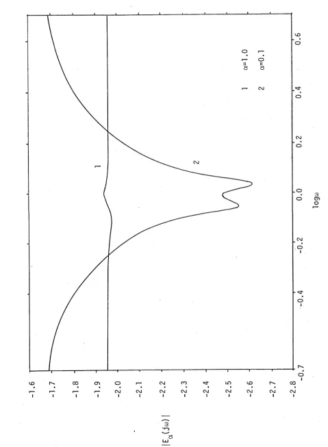
Fig. 1 shows the magnitudes |G | plo tte d against angular frequency f o r two p a r t i c u l a r choices o f a used in t h i s example. Curve 1 has
For convenience o f n o tatio n we denote by E (s) the e rro r system given by E (s) = F(s) - W i(s), where Wi is given by (5.1) and the su b scrip t a
in d ic a te s th a t is the frequency weighting used in (5 .1 ). Note th a t w ith th is n o ta tio n , E-j g(s) is the e r r o r obtained by performing a Hankel-norm approximation o f F(s) with no frequency weighting.
The s in g u la r values o f the system F are:
cFi = .94707, 02= .70013, o 3= .32544, o4 = .08278, F 5 = .00113, a 6 = .00630. This set o f s in g u la r values ind ica tes 07+ as a natural c u t o f f (0 4 / 0 5 - 8)
and so we perform a fo u rth order frequency weighted optimal Hankel-norm approximation o f F(s).
Example ( i ) : a = 0 . 1
With a = 0.1 , the s in g u la r values o f the system K(s) =
[ F (s)Gq 1( - s ) ] _ are: o x = 2.6790, 0 2 = 2.1589, o 3 = .84239, a4 = .19287,
a 5 = .021903, 0 6 = .0011311 . Although each o^ is la rg e r than the
corresponding a . , the new set o f s in g u la r values s t i l l ind ica tes a fo u rth order approximation is ap propriate, (o 4/ o 5 - 9). Fig. 2 shows the magnitude o f the r e s u ltin g e r r o r systems E-| Q(s) and Eg -j (s). We see th a t |Eg 1 ( jco) | is s i g n i f i c a n t l y smaller than |E-j Q( jco) | in a
frequency band about co = 1 .0 and is frequency shaped according
IGq1 1 ( j(jo) I , the o s c i l l a t i o n near co = 1.0 being a ty p ic a l consequence o f
neglecting the unstable p a rt o f the approximation in (2 .1 1 ). Away from co = 1.0, the magnitude o f Eg -|(joo) exceeds s i g n i f i c a n t l y th a t o f
E-] g(jco), however th is is a region where we can to le r a te a less accurate approximation. The method o f frequency weighting has thus performed b e tte r than the d ir e c t Hankel-norm approximation in the pass band o f Gg 1 ( s) and worse in the stop band o f Gq -|(s).
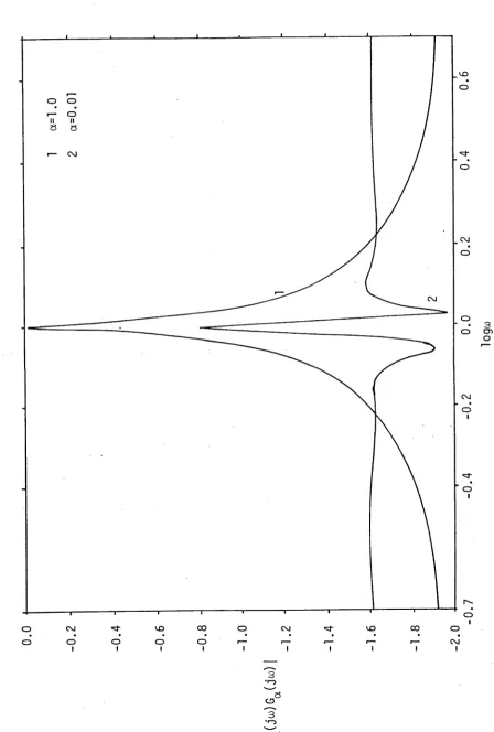
The magnitudes o f the errors in the weighted gains, namely
|| Eg iGq i 1^ - .031 which as expected is close to the lower bound in ( 3 . 3 ) , namely a 5 = .0219. In fa c t the magnitude o f the errors over a l l frequencies is close to t h is value and again in the pass band of Gg i ( s) i t is much less than the e r r o r obtained when E-j g(s) is taken in series with the same frequency weighting.
Example ( i i ) : a = 0.01
With a = .01, the s in g u la r values o f K(s) = [F(s)G g-j(-s)]_ are ö! = 3.6669, o2 = 2.7631 , a 3 = .94358, a 4 = .22032, a b = 024776,
o6 = .001228. Figure 4 shows the magnitudes o f E-j g(s) and E q-j(s) . The shape o f the curve 2 is s im ila r to Fig. 2. Although the minimum e r ro r is s i g n i f i c a n t l y less than th a t f o r Eg -|(s), the o s c i l l a t i o n near oo = 1.0 causes an improvement by only a fa c to r o f about 2 in the pass band o f G q-|(s). The frequency band in which |E g-](jco)|< |E-j g(ju)) |
is less than the corresponding band in Fig. 2. The L°°-norm
||E g-|(ja))G qi ( jw) L can be seen from Fig. 5 to be approximately 0.15 which is much greater than the lower bound in ( 3 . 3 ) , here o 5 = .024226.
In the pass band o f G q- | (s) , the magnitude o f E gi ( jco)G g-|(jw) is s t i l l much less than th a t f o r the d ir e c t Hankel-norm approximation used in series with G g-j(s), (curve 1 o f Fig. 5). The increase in the L°°-norm o f Ea(jaj)Ga( jüü) fo r small a suggests th a t the L°°-norm o f the frequency weighting G (s) needs to be c a r e f u lly chosen to obtain a good compromise
3
Ö
o cn
O
F
ig
1
.
T
h
e
m
a
g
n
itu
d
e
o
f
th
e
fr
e
q
u
e
n
c
y
w
e
ig
h
ti
n
g
[image:32.562.55.520.109.780.2]Fig
5
.
T
he
m
a
g
n
it
u
d
e
s
o
f
th
e
w
e
ig
h
te
d
e
rr
o
rs
corresponding
to
the
ap
pro
xim
ati
on
[image:36.562.72.520.104.768.2]CHAPTER 3
§3.1 INTRODUCTION
The Hankel - nor m a p p r o x i m a t i o n pr obl em o b t a i n e d by i n t r o d u c i n g
f r e q u e n c y w e i g h t i n g in t h e manner d e s c r i b e d in § 2 . 2 , d i f f e r s i n s e v e r a l
i m p o r t a n t r e s p e c t s from t h e d i r e c t Hankel - nor m pr obl em w i t h no
f r e q u e n c y s h a p i n g . Al t hough t h e r ank o f t h e Hankel m a t r i x r ( F G ) i s
p r e s e r v e d , t h e s i n g u l a r v a l u e s a r e o f c o u r s e c o r r u p t e d . T h i s means
oo
t h a t a new s e t o f L and Hankel - nor m e r r o r bounds w i l l be o b t a i n e d .
In t h i s c h a p t e r , we e x p l o r e by how much f r e q u e n c y w e i g h t i n g
change s t h e s i n g u l a r v a l u e s and d e r i v e C° and Hankel - nor m bounds f o r
t h e e r r o r o f t h e r e s u l t i n g s t a b l e a p p r o x i ma t i n g s y s t e m. Th i s w i l l i n
p a r t answer t h e f o l l o w i n g i m p o r t a n t q u e s t i o n s :
( i ) What s a c r i f i c e in a c c u r a c y i s made i n t h e r e s u l t i n g e r r o r i n t h e
L°° and Hankel - nor m me a s u r e s by u s i n g f r e q u e n c y w e i g h t i n g ?
( i i ) How a r e " c l o s e n e s s " i n t h e L°° and Hankel - nor ms r e l a t e d ?
( i i i ) What e f f e c t does t h e c o n s t a n t D o f §2. 5 have on t h e L°° and Ha n kel -
norm bounds?
§3. 2 KNOWN L°°-N0RM BOUNDS
The L°° e r r o r a n a l y s i s wi l l be b a s e d on t h e r e s u l t s o f Gl ove r [ 1 4 ] .
He r e , we p r e s e n t w i t h o u t f u l l p r o o f t h e r e l e v a n t r e s u l t s i n [ 14] . They
oo
r e l a t e t h e L -norm o f a s t a b l e t r a n s f e r f u n c t i o n t o t h e Hankel s i n g u l a r -
v a l u e s o f t h a t f u n c t i o n which a r e assumed f o r c o n v e n i e n c e t o be non-
r e p e a t e d . F i r s t i s a r e p r e s e n t a t i o n Lemma.
Lemma 3.1 L e t F(z) be a s t a b l e , r a t i o n a l t r a n s f e r f u n c t i o n o f
Then there exists a representation of F(z) as
F(z) - D
q+
cjiE
i(
z) + . . . + onEn(z)
( 3 - Dwhere
(1) E-(z) is all-pass and stable for all j
vJ(2) For j = 1... k
(3.2)
has McMillan degree k.
This result is easily proved by recursing on the one-step optimal
Hankel-norm approximation of F(z) while noting that in this case, the
singular values are preserved and the all-pass functions n_/£+ (of §1.5)
are stable.
Lemma 3.2
In addition to the properties of Lemma 3.1, let
F(z) be such that lim F(z) = 0. Then
(1) II ML < 2(qi + . . . + o p )
(2) there exists a constant D such that
(3.3)
1 F
-D0L
< a , + . . . + a n(3.4)
and
(3.5)
Proof
(3.4) is obvious i f DQ is the constant in (3.1).
(3.5)
Although by d e f i n i t i o n , the constant term in the Laurent expansion o f a t r a n s f e r f u n c t i o n plays no p a r t i n det er mi ni ng the optimal Hankel- norm approximation problem, i t i s p os si bl e to add a constant to the s o l u t i o n o f t h i s problem, i n such a way t h a t the o v e r a l l L°°-error i s reduced. This i s the theme o f the f o l l o w i n g r e s u l t .
Lemma 3.3 Let X(z) be the optimal Hankel-norm approximation o f degree k t o the s ta b l e r a t i o n a l t r a n s f e r f u n c t i o n F(z) o f degree n. Then ther e e x i s t s a constant DQ such t h a t :
II F - X. - DoIL <
W F>
+ . 1
i = k+2( 3 . 6 )
n
and II DJI < £ a • ( F)
" k+i 1
( 3 . 7 )
A r where X_ = [X]
§3.3 ERROR ANALYSIS
In t h i s s e c t i o n , we use the r e s u l t s o f §3.2 to der ive upper and lower bounds on the L°°-norm o f the e r r o r f o r the frequency weighted approximation given in §2.3. We also present bounds f o r the norms o f the associated Hankel mat ri ces f o r the frequency weighted case.
The f i r s t r e s u l t i s a growth bound on the s i n g u l a r values o f the system FG i n terms o f those o f the system F.
Lemma 3.4 Let F(z) be a real proper r a t i o n a l and s t a b l e t r a n s f e r f u n c t i o n o f degree n. L et G(z) be a s t a b l e and minimum phase proper t r a n s f e r f u n c t i o n . Then
cri (FG)
where G is as in Definition 2.1, §2.2.
Proof
Because G is real rational, || G^ = || G|^ and
II G'ML = || G-1 |L •
We also have that for any K(z) G L°°, then
II T( K) || = || KL where T(K) is the Toeplitz matrix with symbol
K(z) (see [5 ]).
According to (5.10) of §1.5, || 6 ^ o.(F) =
II G||a.(F) = inf || r(F) - L ||
|| T(G) || > inf || (r(F) - L)T(G) ||
1
L
L
Using Lemma 2.1, §2.2, this is || G^o^(F)> inf || r(FG) - LT( G) ||
Again by Lemma 2.1, 52.2, LT(G) is Hankel and has rank i - 1 , hence
II G||00a i (F) > inf|| r(FG) - A|| = a.(FG)
1
A
Similarly,
|| G'1 ||0O
a 1 ( FG) = inf || F( FG) - L|| || T( G~1) ||
> inf || (r(FG) - D K G ' 1) || > inf || r(F) - LT(G” D ||
L
L
i inf || r(F) - A||
= a • ( F) .
A
1
It i s also possible to relate the singular values of FG to those of FG
by using the results of §1.6.
To do t h i s , we note that FG = FG B where
B = GG- 1i s all- pa ss .
FG is therefore a system with an al l-pass factor.
For sim pli cit y, assume that B has m < n stable poles and m unstable
poles ie G has the same number of zeros and poles.
The results of
Lemma 1.7, §1.6, then translate as follows:
K ( FG) > ° i+m(FG)
i = 1
-•- n
and
o . +m(FG) < o i (FG)
i = 1
. . .
n-m (3.9)
and
o i+m(FG)« o^FG) < o , . m( FG)
i = m + 1 . . . n
For convenience, we r e c a l l the n o t a t i o n o f §2.2 as f o l l o w s : ( i ) ( £, n) i s a Schmidt p a i r o f r(FG) corresponding to a^+-|(FG).
( i i ) X = FG - Sep (3.10)
i s the k - t h or der o f optimal Hankel-norm approxi mation o f FG where o = o ^+-|(FG) and 4>(z) = o _ ( z ) / 6 + (z) , and
( i i i ) W = XG"1 = F - ocpG'1 (3.11)
i s the frequency weighted approximation to the s t a b l e proper system F ( z ) .
We then have a bound on the Hankel matr ices o f F(z) and W(z) as f o l l o w s .
Lemma 3.5 The Hankel mat ri ces r(F) and r(W) s a t i s f y ,
I I C 1 * 11 F(F) ' F(W) 11 « II G - - L (3.12)
a
P r o o f . We have || r(F) - r(W) || = || r(a4>G_ 1) || = cr^oQG"1).
Lemma 3.4 can be a p p l i e d si nce G*1 e H“ so t h a t
öitöc^G'1) < || G_1L o which i s the upper bound. For the lower bound, c o n s i der r(FG) - T(X).
r(FG) - r(x) = (r(F) - r(XG_1))T(G) = (r(F) - r ( w) )t(g)
where we have used Lemma 2 . 1 , §2.2. Thus
II r (FG) - T(X) II = ä « II r(F) - r(w)|| || T(G)|| . However
II T(G)| = || GIL = II GIL •
Remark Using Lemma 3 . 4 , ( 3. 12 ) may be w r i t t e n as
II GIL1 II G' ML1 * 11 r(F) : , (w)l1 < II G' ML I I GL (3.13)
which is in general a looser bound but involves the s in g u la r values o f
r(F).
S u r p r is in g ly , the weighted systems FG and WG have the same separation, in the Hankel-norm as the systems FG and X. We prove th is in the fo llo w in g Lemma.Lemma 3.6 For a l l orders k o f the approximation (3 .1 0 ),
|| r(FG) - r(WG) | | = o . (3.14)
Proof We analyse the a ll-p a s s fun ction ^G_1G.
F(z) has n stable poles. Let G(z) have m stable poles and 1 stable zeros (and only these). G_1G the refore has m stable poles and 1 unstable poles, (j) has in general n+k stable and n-k-1 unstable poles. The d iffe re n c e in number o f stable and unstable poles o f (j)G_1G is therefore (n+m+k) - (n-k-1 +1) = 2k + m - 1 + 1
which is always s* 1. Thus 4>G_1G is an a ll-p a s s fun ction w ith more stable than unstable poles and so by C orollary 1.11, §1.6,
q i( 4)G-1G) = 1. This proves (3 .1 4 ).
We now proceed to derive L°°-norm e r r o r bounds f o r the approximations (3.10) and (3.11) and compare them w ith those in the Hankel-norm.
/V _
Denote as usual by W, the q u a n tity F - ö [(pG- 1 ]_ . According to Lemma 3.1, [o^G- 1 ]_ has a representation as
[acpG- 1 ]_ = ip0 + cfiijn + .. . + ä n+ki^n+k (3.15)
where the ij j . ( j > 1) are a ll-p a s s and stable and we have accorded with
J
the assumption th a t the a\ are not repeated. In the same manner as §2.5, define a frequency weighted approximation WQ to F by
and the e r r o r system EQ by
co
We then have the fo llo w in g bound f o r the L -norm o f E . Lemma 3.7 For the e r r o r EQ o f (3 .1 7 ),
II C 1 < ^ < (n + k ) II G 'M L
(3.17)
(3.18)
where k is the degree o f the approximant (3.10).
/ \ Proof We have th a t r(F) - r(W ) = r(F) - r(W) = r(F) - r(W) By Nehari's theorem,
II r(F) - r(w)|| = || r(F) - r(w0)|| < || F-w0 t = || E0 L so by Lemma 3.5, || EQIj^ > || G|Q*d . By (3 .1 5 ),
II E0 L = II [3d>G~ 1 ]_ - = II 3 ^ ‘ + + ° n+k<Fn+kIL + . . . + 0n+k . Again by Nehari's theorem, = Oj(d<|)G ‘ ) < ||r(Sit>G ' ) ! 5: ollG“ ^ f o r j = 1 . . . n+k. This gives the upper bound o f (3.18). Remark Lemma 3.4 may again be used to give the bounds (3.18) in terms o f a k+-|(F) and (3.18) y ie ld s the upper bound ||EqG ^ < (n+k)a|| G^H G_1|L f o r the weighted system EQG.
Note here th a t the important consequence o f Lemma 3.7 is to demonstrate the existence o f a constant ^ such th a t the upper bound (3.18) is accomplished. The lower bound is in s e n s itiv e to the choice o f the constant. Choosing the constant gives a s u ita b ly small L°° bound on E , however there is no guarantee th a t WQ w i l l be frequency shaped.
For t h i s reason, i t is more s u ita b le to choose the constant D in the expansion o f the form (3.1) f o r [FG]_ ra th e r than i|/ . This is in fa c t the type o f choice th a t is made in the example o f §2.5.
Assumption. We assume in the fo llo w in g th a t lim G"1 (z) = 1. 2 - X »
Let
Wi = W + D
be the frequency weighted approximation to F and
E = F - Wx
the e r ro r system. The constant D is chosen so tha t according to Lemma 3.3,
n
II [ F G ] - X - D L < Z a . ( F G )
k+1 1 and
II DlL
< Z O .(FG) k+1We formulate the L°°-norm bounds f o r E and EG as a theorem.
Theorem 3.8 The L°°-norms o f the e r r o r E and the weighted EG are bounded according to
II G l t ‘ 5 < II E L < K(n,k)
and
II EGIL < II G L K(n,k)
where
K(n,k) (2(n + k) || G-Ml+1)
n
5 + E a • ( FG) k+2 1
(3.19)
(3.20)
(3.21)
(3.22)
e r r o r
(3.23)
Proof Using (3.19) and (3 .2 0 ), W1 = [XG_1]_ + D + F(°°) and E = F - Wi = F - [ ( [FG]_ - 0(J))G_1 - D + F(~) = aL^G"1 ]_ - D so th a t || E11^ £ I a[(|)G_1]_||oo + || . Using Lemma 3.2,
n+k
|| ö[<j>G~1 ] _ L < 2 £ ö i , where are the s in g u la r values o f
a<J>G- 1 . As was shown e a r l i e r (Lemma 3 .7 ), g. £ || G"1^ . n
Combining th is with (3.22) gives || E ^ < 2(n+k)|| G- 1 ^ + £ a i (FG) which is (3 .23). The lower bound in (3.23) follows from Nehari's theorem and Lemma 3.5.
Remark I f in fa c t lim G"1 = 3 where 0 < 3 f 1, the appropriate choice
--- Z -K »
o f constant is ßD instead o f D. In th is case K(n,k) = 2(n + k) || G- 1 ^ n
+ ß E g.(FG) . k+1 1
§3.4 CONCLUSION
In t h is chapter, we have derived weak bounds in the C° and
Hankel-norms f o r the frequency weighting scheme. A p p lic a tio n o f the bounds to the example in §2.5 shows th a t they are indeed weak. For example
when || G L = 10, the s in g u la r values grow by a fa c t o r only a t most 3. With || G ' X = 1, (3.23) gives an upper bound o f 20a whereas the actual e r r o r has an L°°-norm o f approximately 5 (see Fig. 2 ), w hile the
th e o re tic a l upper bound from (3.24) is 200 5, compared to the actual weighted e r r o r L°°-norm o f approximately 2 g.
but as is evidenced in Fig. 2 and Fig. 4, the desired shaping is achieved.
The theory o f §3.3 ind ica tes th a t given a frequency weighting G with || Gll^ > 1, some o f the bounds w i l l be small i f || G"1!^ = 1.
Such a choice f o r the frequency weighting w i l l in general be possible f o r simple weighting shapes o r those th a t emphasise only narrow
frequency bands. The bounds also in d ic a te || G L || G- 1 !^ as an important parameter o f the frequency weighting.