Analysing time course microarray data using Bioconductor: a case study using yeast2 Affymetrix arrays

Open Access

S H O R T R E P O R T

© 2010 Gillespie et al; licensee BioMed Central Ltd. This is an open access article distributed under the terms of the Creative Commons Attribution License (http://creativecommons.org/licenses/by/2.0), which permits unrestricted use, distribution, and reproduction in any medium, provided the original work is properly cited.

Short Report

Analysing time course microarray data using

Bioconductor: a case study using yeast2 Affymetrix

arrays

Colin S Gillespie

*†1,2

_{, Guiyuan Lei}

†1,2

_{, Richard J Boys}

1,2

_{, Amanda Greenall}

2,3

_{and Darren J Wilkinson}

1,2

Abstract

Background: Large scale microarray experiments are becoming increasingly routine, particularly those which track a number of different cell lines through time. This time-course information provides valuable insight into the dynamic mechanisms underlying the biological processes being observed. However, proper statistical analysis of time-course data requires the use of more sophisticated tools and complex statistical models.

Findings: Using the open source CRAN and Bioconductor repositories for R, we provide example analysis and protocol which illustrate a variety of methods that can be used to analyse time-course microarray data. In particular, we highlight how to construct appropriate contrasts to detect differentially expressed genes and how to generate plausible pathways from the data. A maintained version of the R commands can be found at http://www.mas.ncl.ac.uk/ ~ncsg3/microarray/.

Conclusions: CRAN and Bioconductor are stable repositories that provide a wide variety of appropriate statistical tools to analyse time course microarray data.

Introduction

As experimental costs decrease, large scale microarray experiments are becoming increasingly routine, particularly those which track a number of different cell lines through time. This is because time-course information provides valuable insight into the dynamic mechanisms underlying the biological processes being observed. However, a proper statistical analysis of time-course data requires the use of more sophisticated tools and complex statistical models. For example, problems due to multiple comparisons are increased by catering for changing effects over time. In this case study, we demonstrate how to analyse time-course microarray data by investigating a data set on yeast. We dis-cuss issues related to normalisation, extraction of probesets for specific species, chip quality and differential expres-sion. We also discuss network inference in the Additional file 1. The freely available software system R (see [1,2]) has many benefits for analysing data of this type and so

throughout the analysis we give the R commands that pro-duce the numerical/graphical output shown in this paper. A maintained version of the R commands can be found at http://www.mas.ncl.ac.uk/~ncsg3/microarray/.

Description of the data

The data were collected according to the experimental pro-tocol described in [3]. Briefly, three biological replicates were studied on each of a wild-type (WT) yeast strain and a strain carrying the cdc13-1 temperature sensitive mutation (in which telomere uncapping is induced by growth at tem-peratures above around 27°C). These replicates were sam-pled initially at 23°C (at which cdc13-1 has essentially WT telomeres) and then at 1, 2, 3 and 4 hours after a shift to 30°C to induce telomere uncapping. The thirty resulting RNA samples were hybridised to Affymetrix yeast2 arrays. The microarray data are available in the ArrayExpress data-base (see [4]) under accession number E-MEXP-1551 .

Loading microarray data into Bioconductor

Installing Bioconductor and associated packages

Assuming that R is already installed, Bioconductor is fairly straightforward to obtain installation script, viz:

* Correspondence: c.gillespie@ncl.ac.uk

1 _{School of Mathematics & Statistics, Newcastle University, Newcastle upon} Tyne, NE1 7RU, UK

† _{Contributed equally}

>url='http://bioconductor.org/biocLite.R'

>source(url)

> biocLite()

This installs a number of base packages, including affy, affyPLM, limma, and gcrma (see [5-7]). Additional

non-standard packages can also be easily installed. For example, the additional packages needed for this paper can be installed by using

>#From Bioconductor

> biocLite(c('ArrayExpress', 'Mfuzz', 'timecourse', 'yeast2.db', 'yeast2probe'))

>#From cran

>install.packages(c('GeneNet', 'gplots'))

Bioconductor packages are updated regularly on the web and so users can easily update their currently installed pack-ages by starting a new R session and then using

>update.packages(repos = biocinstallRepos())

See [8] for further details on installation.

A list of packages used in this paper is given in the Addi-tional file 1.

Entering data into Bioconductor

The data used in this paper can be downloaded from ArrayExpress into R using the commands

>library(ArrayExpress)

> yeast.raw = ArrayExpress('E-MEXP-1551')

Unfortunately due to changes in the ArrayExpress

web-site, the ArrayExpress package for Bioconductor 2.4

(the default version for R 2.9) produces an error and so we must use the package in Bioconductor 2.5 (the default ver-sion for R 2.10). Details for downloading the latest ArrayExpress package can be found in the Additional file 1. A brief description of the yeast.raw object can be

obtained by using the print (yeast.raw) command:

AffyBatch object

size of arrays = 496 × 496 features (3163 kb) cdf = Yeast_2 (10928 affyids)

number of samples = 30 number of genes = 10928 annotation = yeast2

If the Affymetrix microarray data sets have been down-loaded into a single directory, then the .cel files can be

loaded into R using the ReadAffy command.

Also available from ArrayExpress are the experimental conditions. However, some preprocessing is necessary:

> ph = yeast.raw@phenoData

> exp_fac = data.frame(data order = seq (1, 30),

+ strain = ph@data$

Fac-tor.Value.GENOTYPE.,

+ replicates = ph@data$

Fac-tor.Value.INDIVIDUAL.,

+ tps = ph@data$

Fac-tor.Value.TIME.)

>levels(exp_fac$strain) = c('m', 'w')

> exp_fac = with(exp_fac, exp_fac[order(strain, repli-cates, tps), ])

> exp_fac$replicate = rep(c(1, 2, 3), each = 5, 2)

The data frame exp_fac stores all the necessary

infor-mation, such as strain, time and replicate, which are neces-sary for the statistical analysis.

Note that there are two yeast species on this chip, S. pombe and S. cerevisiae. Also, amongst the 10,928 probe-sets (with each probeset having 11 probe pairs), there are 5,900 S. cerevisiae probesets.

Pre-processing

Extraction of S. cerevisiae probesets

As these microarrays contain probesets for both S. cerevi-siae and S. pombe, we first need to extract the S. cerevicerevi-siae data before normalisation. This can be done by filtering out

the S. pombe data using the s_cerevisiae.msk file

from the Affymetrix website (see [9]). Note that users first need to register with the Affymetrix website before down-loading this file. Also note that in our analysis, the tran-script id i.e. the systematic orf name (obtained from [10]) is used for genes with no name.

We obtain a data frame containing lists of S. cerevisiae genes, probes and transcripts (using the function Extrac-tIDs() in the Additional file 1) as follows

>#Read in the mask file

> s_cer = read.table('s_cerevisiae.msk', skip = 2, string-sAsFactors = FALSE)

> probe_filter = s_cer[[1]]

>source('ExtractIDs.R')

> c_df = ExtractIDs (probe_filter)

We also need to restrict the view of yeast.raw to the

x-and y- coordinates of the S. cerevisiae probesets in the cdf environment by using

>#Get the raw dataset for S. cerevisiae only

>library(affy)

>library(yeast2probe)

>source('RemoveProbes.R')

> cleancdf = cleancdfname(yeast.raw@cdfName) > RemoveProbes(probe_filter, cleancdf, 'yeast2probe')

Note that the commands in RemoveProbes.R are

listed in the Additional file 1. Thus the attributes of

yeast.raw, obtained via print(yeast.raw), are

now

AffyBatch object

size of arrays = 496 × 496 features(3167 kb) cdf = Yeast_2(5900 affyids)

number of samples = 30 number of genes = 5900 annotation = yeast2

Data Quality Assessment

Before any formal statistical analysis, it is important to check for data quality. Initially, we might examine the per-fect and mismatch probe-level data to detect anomalies. Images of the first five arrays can be obtained using

> op = par(mfrow = c(3, 2)) >for(i in 1:5) {

+ plot_title = paste ('Strain:', exp_fac$strain [i], 'Time:', exp_fac$tps [i])

+ d = exp_fac$data_order [i]

+ image(yeast.raw [, d], main = plot_title)

+ }

These commands produce the image shown in the Addi-tional file 1: Figure S2. Data quality can be assessed by examining such images for anything that appears non-ran-dom such as rings, shadows, lines and strong variations in shade. The images for our data set do not appear to have any non-random structure and so data quality is probably high.

Another useful quality assessment tool is to examine den-sity plots of the probe intensities. The command

> d = exp_fac$data_order[1:5]

>hist(yeast.raw[, d], lwd = 2, ylab = 'Density', xlab = 'Log (base 2) intensities')

produces the image shown in the Additional file 1: Figure S3. Typically, differences in spread and position are cor-rected by normalisation. However, the appearance of signif-icant multi-modality in the distribution or many outlying observations are indicative of poor data quality.

Other exploratory data analysis techniques that should be carried include MAplots, where two microarrays are com-pared and their log intensity difference for each probe on each gene are plotted against their average. Also of interest is to examine RNA degradation (see [6]), although [11] cast some doubt over the validity of this method. For details on how to carry out both of these methods in R, see [12,13] for detailed instructions.

Normalising Microarray Data

There are number of methods for normalising microarray data. Two of the most popular methods are GeneChip RMA (GCRMA) and Robust Multiple-array Average (RMA); see [14,15]. Essentially, GCRMA and RMA differ in how they deal with background noise, with GCRMA using a more sophisticated correction algorithm. However, the approach adopted by GCRMA means that it can be time-consuming to use with large data sets in contrast to RMA. A potential drawback of using RMA is that it assumes that the overall levels of expression are similar for each array. However this assumption may be invalid if, for example, mutant cells have a radically different level of transcriptional activity than the WT. For further information regarding normalising microarray data sets, see for example [16,17].

Since we have thirty microarray data sets and believe that the levels of transcriptional activity are similar across strains, we will use the RMA normalisation method. This technique normalises across the set of hybridizations at the probe level. The data can be normalised via

> yeast.rma = rma(yeast.raw)

> yeast.matrix = exprs(yeast.rma) [, exp_fac$data_order] > cnames = paste(exp_fac$strain, exp_fac$tps, sep = ' ')

>colnames(yeast.matrix) = cnames

> exp_fac$data_order = 1:30

The normalisation procedure consists of three steps: model-based background correction, quantile normalisation and robust averaging. The aim of the quantile normalisation is to make the distribution of probe intensities for each array in a set of arrays the same. We illustrate its effect by studying boxplots of the raw S. cerevisiae data against their normalised counterparts values, shown in the Additional file 1: Figure S4. Boxplots provide a useful graphical view of data distributions and contain their median, quartiles,

maximum and minimum values. The boxplot command

is in the affyPLM package and so the figure is produced

by using

>library(affyPLM)

>par(mfrow = c(1, 2)) >#Raw data intensities

>boxplot(yeast.raw, col = 'red', main="")

>#Normalised intensities

>boxplot(yeast.rma, col ='blue')

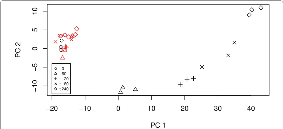
Principal Component Analysis

Principal component analysis (PCA) is useful in explor-atory data analysis as it can reduce the number of variables to consider whilst still retaining much of the variability in the data. In particular, PCA is useful for identifying patterns in the data. Essentially, principal components partition the data into orthogonal linear components which explain dif-ferent contributions to the variability in the data. The first component explains the largest contribution to variability in the original dataset, that is, retains most information, with the second component explaining the next largest contribu-tion to variability, and so on. The following commands cal-culate the principal components

> yeast.PC = prcomp(t(yeast.matrix)) > yeast.scores = predict(yeast.PC) which we can then plot using

>#Plot of the first two principal components >plot(yeast.scores [, 1], yeast.scores [, 2],

+ xlab = 'PC 1', ylab = 'PC 2',

+ pch = rep(seq (1, 5), 6),

+ col = as.numeric(exp_fac$strain))

>legend(-20, -4, pch = 1:5, cex = 0.6, c('t 0', 't 60', 't 120',

't 180', 't 240'))

strain. In particular, mutant samples are clustered by their time points; for example, the three mutant replicates at time point 4 are clustered at the bottom right of the figure.

Identifying differentially expressed genes

In this experiment, interest lies in differences in gene expression over time between the wild-type and mutant yeast strains. It is expected that the wild-type expression level is independent of time. Also we anticipate that the mutant expressions at time t = 0 are the same as the wild-type expression level. This hypothesis is supported by the PCA plot in Figure 1.

There are currently two main packages available to detect differentially expressed genes using this kind of data: the

timecourse package and the limma package. We

illus-trate how to analyse these data using both packages.

Using the timecourse package

This package assesses treatment differences by comparing time-course mean profiles allowing for variability both within and between time points. It uses the multivariate empirical Bayes model proposed by [18].

Further details of the timecourse package can be

found in [19]. After installing the timecourse library,

we construct a size matrix describing the replication

structure using

>library(timecourse)

> size = matrix(3, nrow = 5900, ncol = 2)

To extract a list of differentially expressed we calculate the Hotelling statistic via

> c.grp = as.character(exp_fac$strain) > t.grp = as.numeric(exp_fac$tps)

> r.grp = as.character(exp_fac$replicate)

> MB.2D = mb.long(yeast.matrix, times = 5, method = '2', reps = size,

+ condition.grp = c.grp, time.grp =

t.grp, rep.grp = r.grp)

The top (say) one hundred genes can be extracted via > gene_positions = MB.2D$pos.HotellingT2 [1:100] > gnames = rownames(yeast.matrix)

> gene_probes = gnames[gene_positions]

The expression profiles can also be easily obtained. The profile for the top ranked expression is found using

> plotProfile(MB.2D, ranking = 1, gnames =

rownames(yeast.matrix))

and is shown in the Additional file 1: Figure S5.

Using the limma package

The limma package uses the moderated t-statistic

described by [7,20]. The function lmFit within the

limma library fits a linear model for each gene for a given

series of arrays, where the coefficients of the fitted models describe the differences between the RNA sources hybri-dised to the arrays. Precisely, we fit the model E [yg] = Xαg,

where yg = (yg,1, ..., yg, n)T contains the expression values for

gene g across the n arrays, X is a design matrix which describes key features of the experimental design used and αg is the coefficient vector for gene g. In the analysis

stud-ied here, the yeast data consists of data from n = 30 arrays. The entries in the columns of X depend on the experimental design used: there are two yeast strains (mutant and wild type), each measured at five separate time points, and we are interested in comparing the gene expressions between mutant and wild type strains over time. Thus we seek a

[image:4.595.56.539.502.722.2]

T2

Figure 1 A plot of the first two principal components. The red symbols correspond to the wild-type strain.

−20

−10

0

10

20

30

40

−10

−5

0

5

10

PC 1

PC 2

ear model describing the ten strain × time combinations by determining values for the ten coefficients in the coefficient vector α_g. We will label these ten coefficients as ('m0', 'm60, 'm120', 'm180', 'm240', 'w0', 'w60', 'w120', 'w180', 'w240'), where the first five coefficients represent the levels of the mutant strain at time points t = 0, 1, 2, 3, 4 and the remain-ing five coefficients are the equivalent versions for the wild type strain. Statistically speaking, the model has a single factor with ten levels. The design matrix X links these fac-tors to the data in the arrays by having zero entries except when an array contributes an observation to a particular strain × time combination. For example, array 26 measures the expression of the first wild type microarray at time t = 0 and so contributes an observation to level 'w0', the sixth strain × time combination. Thus the entry in row 26, col-umn 6 of the design matrix X(26, 6) = 1. Further, the arrays are arranged in groups of three replicates. Thus the overall

experimental structure (expt_structure below) has

three arrays on level 'm0', then three arrays on 'm60', and so on. Setting up the factor levels and the design matrix is done in R by using

>library(limma)

> expt_structure = factor(colnames(yeast.matrix)) >#Construct the design matrix

> X = model.matrix(~0 + expt_structure)

>colnames(X) = c('m0', 'm60', 'm120', 'm180', 'm240',

'w0', 'w60', 'w120', 'w180', 'w240')

and then the coefficient vector α_g is estimated via the command

>lm.fit = lmFit(yeast.matrix, X)

Determining the differentially expressed genes amounts to studying contrasts of the various strain × time levels, as described by a contrast matrix C. For these data, we are mainly interested in differences at the later time points, and so a possible set of contrasts to investigate is that of differ-ences between the mutant and wild type strains at each time

point, that is, ('m60-w60', 'm120-w120',

'm180-w180', 'm240-w240'). The limma package

allows complete flexibility over the choice of contrasts, however this necessarily includes an additional level of complexity. The values in the coefficient vector of con-trasts, β_g = CT_α

g for gene g, describe the size of the

differ-ence between strains at each time point. The relevant R commands are

> mc = makeContrasts('m60-w60', 'm120-w120', 'm180-w180', 'm240-w240', levels = X)

> c.fit = contrasts.fit(lm.fit, mc) > eb = eBayes(c.fit)

The final command uses the eBayes function to produce

moderated t-statistics which assess whether individual con-trast values βgj are plausibly zero, corresponding to no

sig-nifficant evidence of a difference between strains at time point j. The moderated t-statistic is constructed using a

shrinkage approach and so is not as sensitive as the standard t-statistic to small sample sizes. It also gives a moderated F-statistic which can be used to test whether all contrasts are zero simultaneously, that is, whether there is no difference between strains at all time points.

Ranking differentially expressed genes

There are a number of ways to rank the differentially expressed genes. For example, they can be ranked accord-ing to their log-fold change

>#see help(toptable) for more options > toptable(eb, sort.by = 'logFC') or by using F-statistics

> topTableF(eb)

The advantage of using F-statistics over the log fold change is that the F-statistic takes into account variability and reproducibility, in addition to fold-change.

Our analysis is based on a large number of statistical tests, and so we must correct for this multiple testing. In our example we use the (very) conservative Bonferroni correc-tion since we have a large number of differentially expressed genes and the resulting corrected list is still long. Another common method of correcting for multiple testing is to use the false discovery rate (fdr) (use the command

?p.adjust to obtain further details). The following

com-mands rank genes according to their (corrected) F-statistic p-value and annotates the output by indicating the direction of the change for each contrast for each gene: +1 for up-reg-ulated expression (mutant type having higher expression than wild type at a particular time point), -1 for down-regu-lated expression and 0 for no significant change.

> modFpvalue = eb$F.p.value

>#Change 'bonferroni' to 'fdr' to use the false discovery rate as a cut-off

> indx = p.adjust(modFpvalue, method = 'bonferroni') < 0.05

> sig = modFpvalue[indx]

>#No. of sig. differential expressed genes > nsiggenes = length(sig)

> results = decideTests(eb, method = 'nestedF') > modF = eb$F

> modFordered = order(modF, decreasing = TRUE) >#Retrieve the significant probes and genes

> c_rank_probe = c_df$probe [modFordered

[1:nsiggenes]]

> c_rank_genename = c_df$genename [modFordered [1: nsiggenes]]

>#Create a list and write to a file

> updown = results[modFordered [1:nsiggenes],]

>write.table(cbind(c_rank_probe, c_rank_genename,

updown),

+ file = 'updown.csv', sep = ',', row.names =

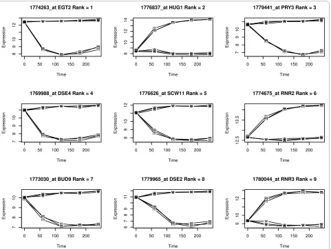
The following code (adapted from lecture material found at [13]) plots the time course expression for the top one hundred differentially expressed genes according to their F-statistic (see Figure 2).

>#Rank of Probesets, also output gene names >par(mfrow = c (3, 3), ask = TRUE, cex = 0.5) >for (i in 0:99){

+ indx = rank(modF) == nrow(yeast.matrix) -i +

+ id = c_df $probe [indx] + name = c_df $genename [indx]

+ genetitle = paste (sprintf ('%. 30s', id), sprintf ('%. 30s', name), 'Rank =', i +1)

+

+ exprs.row = yeast.matrix [indx, ] +

+ plot (0, pch = NA, xlim = range(0, 240), ylim =

range(exprs.row), ylab = 'Expression',

+ xlab = Time, main = genetitle)

+

+ for (j in 1:6){

+ pch_value = as.character (exp_fac$strain [5 * j])

+ points (c (0, 60, 120, 180, 240), exprs.row [(5 *

j-4):(5 * j)], type = 'b', pch = pch_value) + }

+ }

When interpreting rank orderings based on statistical sig-nificance, it is important to bear in mind that a statistically significant differential expression is not always biologically meaningful. For example, Figure 2 contains RNR2. This gene is highly significant because of low variation in its time course. However the actual difference in expression levels between wild-type and mutant stains is relatively small. We address this problem in the next section.

Comparison of the timecourse and limma packages Both packages have different strengths. One advantage of the timecourse package over the limma package is that

[image:6.595.60.541.362.724.2]

it allows for correlation between repeated measurements on the same experimental unit, thereby reducing false positives and false negatives; these false positives/negatives are a significant problem when the variance-covariance matrix is

Figure 2 Time course expression levels for the top 9 differentially expressed genes, ranked by their F-statistic.

0 50 100 150 200

8

9

10

12

1774263_at EGT2 Rank = 1

Time Expression m m m m m m m m m m m m

m m m

w w w w w

w w w w w

w w w w w

0 50 100 150 200

8

1

01

21

4

1776837_at HUG1 Rank = 2

Time

Expression

m m

m m m

m m

m m m

m m

m m m

w w _{w w w}

w w _w

w w

w w _{w w w}

0 50 100 150 200

789

1

0

1779441_at PRY3 Rank = 3

Time Expression m m m m m m m m m m m m

m _m m

w w w w w

w w w w w

w w w w

w

0 50 100 150 200

789

1

0

1769988_at DSE4 Rank = 4

Time Expression m m m m m m m

m m m

m

m

m m

m

w w

w w w

w w w

w w

w w w w

w

0 50 100 150 200

8

9

10

12

1776626_at SCW11 Rank = 5

Time

Expression

m

m

m m m

m

m

m m m

m

m

m _{m m}

w w

w w w

w

w w w w

w w

w w w

0 50 100 150 200

12.5

13.5

1774675_at RNR2 Rank = 6

Time

Expression

m m

m m m

m m m m m m m

m m m

w _w

w w w

w _{w w} w w

w _w

w w w

0 50 100 150 200

789

1

0

1773030_at BUD9 Rank = 7

Time

Expression

m

m

m m m

m

m

m m m

m

m

m _{m m}

w w

w w w

w w w w

w

w w w w

w

0 50 100 150 200

6789

1

1

1779965_at DSE2 Rank = 8

Time

Expression

m

m

m m m

m m m m m m m

m _{m m}

w w

w w w

w w

w w w

w

w w w w

0 50 100 150 200

91

0

1

2

1780044_at RNR3 Rank = 9

Time

Expression _m

m

m m m

m m

m m m

m m

m m m

w w

w w w

w

w _w w w

w

w _{w w}

poorly estimated. An advantage of the limma package is

that it allows more flexibility by allowing users to construct different contrasts. In general we might expect both pack-ages to produce fairly similar lists of say the top 100 probe-sets. In the analysis of the yeast data, we can determine the overlap of the top 100 probesets by using

> N = 100

> gene_positions = MB.2D$pos.HotellingT2 [1:N] > tc_top_probes = gnames [gene_positions]

> lm_top_probes = c_df$probe [modFordered [1:N]]

>length(intersect(tc_top_probes, lm_top_probes))

The result is a moderately large overlap of fifty-three probesets. We note that changing the ranking method in the

limma package also yields similar results as those given by

the timecourse library.

Two fold-change list

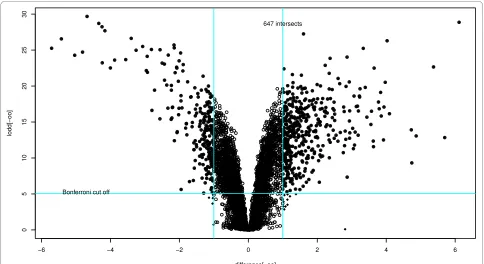
When looking for "interesting" genes it can be helpful to restrict attention to those differential expressed that are both statistically significant and of biological interest. This objective can be achieved by considering only significant genes which show, say, at least a two-fold change in their expression level. This gene list is obtained using the follow-ing code (adapted from [12])

>#Obtain the maximum fold change but keep the sign > maxfoldchange = function(foldchange)

+ foldchange[which.max(abs(foldchange))] > difference = apply(eb$coeff, 1, maxfoldchange) > pvalue = eb$F.p.value

> lodd = log10(pvalue) >#hfc: high fold-change

> nd = (abs(difference) >log (2, 2))

> ordered_hfc = order(abs(difference), decreasing = TRUE)

> hfc = ordered_hfc[1: length(difference [nd])] > np = p.adjust(pvalue, method = ' bonferroni') < 0.05 >#lpv: low p value(large F-value)

> ordered_lpv = order(abs(pvalue), decreasing = FALSE)

> lpv = ordered_lpv[1: length (pvalue [np])] > oo = union(lpv, hfc)

> i i = intersect(lpv, hfc)

Figure 3 contains a "volcano" plot which illustrates the effect of using different levels of fold change and signifi-cance thresholds. The figure is produced by using the fol-lowing code

>#Construct a volcano plot using moderated F-statistics >par(cex = 0.5)

>plot(difference[-oo], lodd[-oo], xlim = range (differ-ence), ylim = range(lodd))

>points(difference[hfc], lodd[hfc], pch = 18)

>points(difference[lpv], lodd[lpv], pch = 1)

>#Add the cut - off lines

>abline(v = log (2, 2), col = 5); abline (v = - log (2, 2),

col = 5)

>abline (h = -log10 (0.05/5900), col = 5)

>text (min(difference) + 1, -log10 (0.05/5900) + 0.2,

[image:7.595.56.540.454.718.2]

'Bonferroni cut off')

Figure 3 Volcano plot showing the Bonferroni cut-off and the two-fold change.

−6 −4 −2 0 2 4 6

0

5

10

15

20

25

30

difference[−oo]

lodd[−oo]

Bonferroni cut off

>text (1, max(lodd) - 1, paste (length (i i), 'intersects'))

Cluster Analysis

Biological insight can be gained by determining groups of differentially expressed genes, that is, groups of genes which increase or decrease simultaneously. This can be achieved by using cluster analysis.

Traditional cluster analysis

In this section, we separate the top fifty differentially expressed genes into groups of similar pattern (clusters). Clearly different genes will have different overall levels of expression and so we first standardise their measurements by taking the expression level of the mutant strain (at each time point) relative to the wild-type at time t = 0:

> c_probe_data = yeast.matrix [ii,] >#Average of WT

> wt_means = apply(c_probe_data [, 16:30], 1, mean) > m = matrix(nrow = dim(c_probe_data) [1], ncol = 5) >for (i in 1:5) {

+ mut_rep = c(i, i+5, i +10)

+ m [, i] = apply(c_probe_data [, mut_rep], 1, mean) - wt_means

+ }

>colnames(m) = sort(unique(exp_fac$tps))

The heatmap in Figure 4 is obtained by using the function

heatmap.2 from the library gplots via the following

code

>library(gplots)

>#Cluster the top 50 genes

> heatmap.2 (m [1:50,], dendrogram = 'row', Colv = FALSE, col = greenred (75),

+ key = FALSE, keysize = 1.0, symkey =

FALSE, density.info = ' none',

+ trace = 'none', colsep = rep(1:10), sepcolor

= 'white', sepwidth = 0.05,

+ hclustfun = function (c){hclust(c, method = 'average')},

+ labRow = NA, cexCol = 1)

Figure 4 shows the relative expression levels for the mutant strain at each time point ('0', '60', '120', '180', '240'). As expected, the relative expression levels at time t = 0 are very similar. However, as time progresses, groupings of genes appear whose levels are up-regulated (red) or down-regulated (green). Note that the intensity of the colour cor-responds to the magnitude of the relative expression. Gene names appear on the right side of the figure and on the left side, the cluster dendrogram shows which genes have simi-lar expression. The dendrogram suggests that there are per-haps six to ten clusters.

Soft clustering

Soft clustering methods have the advantage that a probe can be assigned to more than one cluster. Furthermore, it is

pos-sible to grade cluster membership within particular group-ings. Soft clustering is considered more robust when dealing with noisy data; for more details see [21,22]. The

Mfuzz package implements soft clustering using a fuzzy

c-means algorithm. Analysing the data for c = 8 clusters is achieved by using

>library(Mfuzz)

> tmp_expr = new('ExpressionSet', exprs = m) > cl = mfuzz(tmp_expr, c = 8, m = 1.25)

> mfuzz.plot(tmp_expr, cl = cl, mfrow = c (2, 4), new.window = FALSE)

Of course, it is usually not clear how many clusters there are (or should be) within a dataset and so the sensitivity of conclusions to the choice of number of clusters (c) should always be investigated. For example, if c is chosen to be too large then some clusters will appear sparse and this might suggest choosing a smaller value of c. Figure 5 shows the profiles of the eight clusters obtained from the Mfuzz pack-age. The probes present within each cluster can be found by using

> cluster = 1 > cl [[4]][, cluster]

Conclusion

The response to telomere uncapping in cdc13-1 strains was expected to share features in common with responses to cell cycle progression, environmental stress, DNA damage and other types of telomere damage. The statistical analysis determined lists of probesets associated with genes involved in all of these processes. The techniques used focussed on making best use of the temporal information in time-course data. The use of cdc13-1 strains, which uncap telomeres quickly and synchronously, also allowed the identification of genes involved in the acute response to telomere damage. This case study has demonstrated the power of R/Bioconductor to analyse time-course microar-ray data. Whilst the statistical analysis of such data is still an active research area, this paper presents some of the cut-ting-edge tools that are available to the life science commu-nity. All software discussed in this article is free, with many of the packages being open-source and subject to on-going development.

Additional material

Competing interests

The authors declare that they have no competing interests.

Authors' contributions

AG conducted the microarray experiments. All authors participated in the anal-ysis of the data and in the writing of the manuscript.

[image:9.595.56.538.98.326.2]

Figure 4 Clustering of the top fifty differentially expressed genes. Red and green correspond to up- and down-regulation respectively.

0

60

120

180

240

Figure 5 Eight clusters obtained using the Mfuzz package.

Cluster 1

Time

Expression changes

1 2 3 4 5

−4

−2

0

Cluster 2

Time

Expression changes

1 2 3 4 5

−2.0

−0.5

Cluster 3

Time

Expression changes

1 2 3 4 5

−1

0

1

2

Cluster 4

Time

Expression changes

1 2 3 4 5

−0.5

1.0

Cluster 5

Time

Expression changes

1 2 3 4 5

−1

1

3

5

Cluster 6

Time

Expression changes

1 2 3 4 5

−5

−3

−1

Cluster 7

Time

Expression changes

1 2 3 4 5

−3

−1

1

Cluster 8

Time

Expression changes

1 2 3 4 5

[image:9.595.58.539.441.727.2]

Acknowledgements

We wish to thank Dan Swan (Newcastle University Bioinformatics Support Unit) and David Lydall for helpful discussions. The authors are affiliated with the Cen-tre for Integrated Systems Biology of Ageing and Nutrition (CISBAN) at Newcas-tle University, which is supported jointly by the Biotechnology and Biological Sciences Research Council (BBSRC) and the Engineering and Physical Sciences Research Council (EPSRC).

Author Details

1_{School of Mathematics & Statistics, Newcastle University, Newcastle upon} Tyne, NE1 7RU, UK, 2_{Centre for Integrated Systems Biology of Ageing and} Nutrition (CISBAN), Newcastle University, UK and 3_{Institute for Ageing and} Health, Newcastle University, Campus for Ageing and Vitality, Newcastle upon Tyne, NE4 5PL, UK

References

1. R Development Core Team: R: A Language and Environment for Statistical Computing 2009 [http://www.r-project.org]. Vienna, Austria

2. Gentleman RC, Carey VJ, Bates DM, Bolstad B, Dettling M, Dudoit S, Ellis B, Gautier L, Ge Y, Gentry J, Hornik K, Hothorn T, Huber W, Iacus S, Irizarry R, Leisch F, Li C, Maechler M, Rossini AJ, Sawitzki G, Smith C, Smyth G, Tierney L, Yang JYH, Zhang J: Bioconductor: open software development for computational biology and bioinformatics. Genome Biology 2004,

5:R80.

3. Greenall A, Lei G, Swan DC, James K, Wang L, Peters H, Wipat A, Wilkinson DJ, Lydall D: A genome wide analysis of the response to uncapped telomeres in budding yeast reveals a novel role for the NAD+ biosynthetic gene BNA2 in chromosome end protection. Genome Biology 2008, 9:R146.

4. Parkinson H, Kapushesky M, Kolesnikov N, Rustici G, Shojatalab M, Abeygunawardena N, Berube H, Dylag M, Emam I, Farne A, Holloway E, Lukk M, Malone J, Mani R, Pilicheva E, Rayner TF, Rezwan F, Sharma A, Williams E, Bradley XZ, Adamusiak T, Brandizi M, Burdett T, Coulson R, Krestyaninova M, Kurnosov P, Maguire E, Neogi SG, Rocca-Serra P, Sansone SA, Sklyar N, Zhao M, Sarkans U, Brazma A: ArrayExpress update-from an archive of functional genomics experiments to the atlas of gene expression. Nucleic Acids Research 2009, 37:D868-72. 5. Gautier L, Cope L, Bolstad BM, Irizarry RA: affy-analysis of Affymetrix

GeneChip data at the probe level. Bioinformatics (Oxford, England) 2004,

20(3):307-15.

6. Bolstad BM, Collin F, Brettschneider J, Simpson K, Cope L, Irizarry RA, Speed TP: Bioinformatics and Computational Biology Solutions Using R and Bioconductor New York: Springer-Verlag. Statistics for Biology and Health; 2005:33-48.

7. Smyth GK: Limma: linear models for microarray data. In Bioinformatics and Computational Biology Solutions using R and Bioconductor Edited by: Gentleman R, Carey V, Dudoit S, R Irizarry WH. New York: Springer; 2005:397-420.

8. Bioconductor: Installation instructions. [http://www.bioconductor.org/ docs/install].

9. Pombe and Cerevisiae Filter [http://www.affymetrix.com/Auth/ support/downloads/mask_files/s_cerevisiae.zip]

10. Yeast Annotation File [http://www.affymetrix.com/Auth/analysis/ downloads/na24/ivt/Yeast_2.na24.annot.csv.zip]

11. Archer KJ, Dumur CI, Joel SE, Ramakrishnan V: Assessing quality of hybridized RNA in Affymetrix GeneChip experiments using mixed-effects models. Biostatistics (Oxford, England) 2006, 7(2):198-212. 12. Gregory Alvord W, Roayaei JA, Quiñnones OA, Schneider KT: A microarray

analysis for differential gene expression in the soybean genome using Bioconductor and R. Briefings in Bioinformatics 2007, 8:415-31. 13. Analysis of Gene Expression Data Short Course, JSM2005 [http://

bioinf.wehi.edu.au/marray/jsm2005/]

14. Irizarry RA, Hobbs B, Collin F, Beazer-Barclay YD, Antonellis KJ, Scherf U, Speed TP: Exploration, normalization, and summaries of high density oligonucleotide array probe level data. Biostatistics (Oxford, England) 2003, 4:249-64.

15. Wu Z, Irizarry RA, Gentleman R, Martinez-Murillo R, Spencer R: A Model Based Background Adjustment for Oligonucleotide Expression Arrays. Journal of the American Statistical Association 2004, 99:909-917.

16. Harr B, Schlötterer C: Comparison of algorithms for the analysis of Affymetrix microarray data as evaluated by co-expression of genes in known operons. Nucleic Acids Research 2006, 34:e8.

17. Labbe A, Roth MP, Carmichael PH, Martinez M: Impact of gene expression data pre-processing on expression quantitative trait locus mapping. BMC Proceedings 2007, 1(Suppl 1):S153.

18. Tai YC, Speed TP: A multivariate empirical Bayes statistic for replicated microarray time course data. The Annals of Statistics 2006, 34:2387-2412. 19. Tai YC: timecourse: Statistical Analysis for Developmental Microarray Time

Course Data 2007 [http://www.bioconductor.org].

20. Smyth GK: Linear models and empirical Bayes methods for assessing differential expression in microarray experiments. Statistical Applications in Genetics and Molecular Biology 2004, 3:Article3.

21. Futschik ME, Carlisle B: Noise-robust soft clustering of gene expression time-course data. Journal of Bioinformatics and Computational Biology 2005, 3:965-88.

22. Futschik M: Mfuzz: Soft clustering of time series gene expression data 2007 [http://itb.biologie.hu-berlin.de/~futschik/software/R/Mfuzz/index.html].

doi: 10.1186/1756-0500-3-81

Cite this article as: Gillespie et al., Analysing time course microarray data

using Bioconductor: a case study using yeast2 Affymetrix arrays BMC Research Notes 2010, 3:81

Received: 6 July 2009 Accepted: 19 March 2010 Published: 19 March 2010

This article is available from: http://www.biomedcentral.com/1756-0500/3/81 © 2010 Gillespie et al; licensee BioMed Central Ltd.

This is an open access article distributed under the terms of the Creative Commons Attribution License (http://creativecommons.org/licenses/by/2.0), which permits unrestricted use, distribution, and reproduction in any medium, provided the original work is properly cited.