T E C H N I C A L N O T E
Open Access
MLEP: an R package for exploring the
maximum likelihood estimates of penetrance
parameters
Yuki Sugaya
Abstract
Background: Linkage analysis is a useful tool for detecting genetic variants that regulate a trait of interest, especially genes associated with a given disease. Although penetrance parameters play an important role in determining gene location, they are assigned arbitrary values according to the researcher’s intuition or as estimated by the maximum likelihood principle. Several methods exist by which to evaluate the maximum likelihood estimates of penetrance, although not all of these are supported by software packages and some are biased by marker genotype information, even when disease development is due solely to the genotype of a single allele.
Findings: Programs for exploring the maximum likelihood estimates of penetrance parameters were developed using the R statistical programming language supplemented by external C functions. The software returns a vector of polynomial coefficients of penetrance parameters, representing the likelihood of pedigree data. From the likelihood polynomial supplied by the proposed method, the likelihood value and its gradient can be precisely computed. To reduce the effect of the supplied dataset on the likelihood function, feasible parameter constraints can be introduced into maximum likelihood estimates, thus enabling flexible exploration of the penetrance estimates. An auxiliary program generates a perspective plot allowing visual validation of the model’s convergence. The functions are collectively available as the MLEP R package.
Conclusions: Linkage analysis using penetrance parameters estimated by the MLEP package enables feasible localization of a disease locus. This is shown through a simulation study and by demonstrating how the package is used to explore maximum likelihood estimates. Although the input dataset tends to bias the likelihood estimates, the method yields accurate results superior to the analysis using intuitive penetrance values for disease with low allele frequencies. MLEP is part of the Comprehensive R Archive Network and is freely available at http://cran.r-project.org/ web/packages/MLEP/index.html.
Keywords: Penetrance, Maximum likelihood estimate, Linkage analysis, Polynomial evaluation
Findings Background
Linkage analysis remains a useful tool for detecting genetic variants that regulate a trait of interest, especially genes associated with a given disease. The likelihood of pedigree data plays an important role in this analysis; however, the entire likelihood function embodies func-tions of recombination fracfunc-tions, penetrance parameters,
Correspondence: [email protected]
School of Fundamental Science and Technology, Keio University, Yokohama, Japan
and disease and marker allele frequencies. Such complex-ity can be reduced by varying only the recombination frac-tion, assigning fixed values to the other parameters. This allows the multivariate function to be expressed in terms of a single variable (the recombination fraction). The ratio of the univariate likelihood, the so-called LOD score [1], is then computed to map disease loci, rather than max-imizing the likelihood itself. For a small recombination fraction, a high LOD score (greater than 3) implies that the disease locus is located near the markers employed in the analysis. Assuming the conditional parameters to achieve such high LOD scores depends largely on the researcher’s intuition.
Linkage analysis is hindered by the lack of useful tools and programs for the parameter estimation, although sev-eral methods for maximum likelihood estimate (MLE) of penetrance have been proposed. Two types of pene-trance estimation are described in the literature. The first is based on pedigree data with marker genotype informa-tion; for which the likelihood ispθ(aV,mV), whereaVand
mV represent observations of affected status and marker genotypes respectively, for a set of pedigree members V. The parameter vectorθ contains penetrance parame-ters, disease allele frequency, and recombination fraction, so that maximum likelihood estimates are obtained for all parameters simultaneously. The evaluated maximum likelihood estimate of penetrance parameters is therefore affected by the estimates of both recombination frac-tion and disease allele frequency. Because penetrance and marker genotype observations are independent (unless the marker and disease loci are extremely close), the method is not suitable for penetrance estimation in which a single disease allele determines whether the disease will manifest. This method has been shown in GENEHUNTER-MODSCORE [2-5] in which the ratio of the likelihood, or mod score function [6], can be max-imized in practice. The second approach considers the likelihood of affected status; that is, the likelihood is expressed as pθ˜(aV). Maximized likelihood is a func-tion of the penetrance parameters alone, θ˜, for a par-ticular case. Wang et al. [7] formalized the likelihood using Bayes theorem and proposed a method for esti-mating the penetrance parameter, but which functions only when a carrier of a disease allele develops the dis-ease. The estimate was applied to a dominant disease; therefore, it is not applicable to diseases which man-ifest via other modes of inheritance. Swartz et al. [8] developed three different kinds of estimators and com-pared their efficiencies by a ratio of asymptotic variance of one estimator to another. The efficiency was com-puted and illustrated by a perspective plot using the program Maple [9,10], but these methods are limited to sib pairs. The methods have not been packaged as freely available software, hence are not immediately applicable to wider data analysis. A known problem with pene-trance estimation methods is that their estimates depend largely on the collected pedigrees. However, these sec-ond approaches ensure robust estimates by using multiple sets of previously-recorded pedigree data for the same disease to estimate parameters, which are available from the literature; the marker genotype information is not available.
Our proposed method belongs to the second class of penetrance estimation. The likelihood pθ˜(aV) can
be explicitly expressed as a polynomial of penetrance parameters, and the evaluation measure is a vector of
likelihood polynomial coefficients. More precisely, the coefficient vectors for each pedigree are evaluated by their independence property. Once the likelihood vectors have been computed, the problem reduces to one of optimiza-tion. The maximum likelihood estimates of penetrance parameters are then readily obtained by maximizing the likelihood using standard statistical software. We have developed programs to explore the maximum likelihood estimates of penetrance parameters using R statistical pro-gramming language [11] supplemented with external C functions. The main function of the package evaluates the list of likelihood coefficient vectors. The software enables flexible exploration of the penetrance estimates by cal-culating the likelihood value and its gradient precisely, and passing them to an optimization function. The explo-ration is rendered more powerful if feasible parameter constraints can be incorporated in the maximum likeli-hood evaluation. Another advantage of our method is that it provides visual validation of convergence, in the form of perspective plots of the likelihood surface. All of the func-tions are available in the MLEP R package. Although the MLEP estimates are biased by the collected disease pedi-gree data, we show that they can more accurately identify a disease locus than can analysis based on intuitive pene-trance values provided that both true and assumed disease allele frequency are small. The MLEP package is part of the Comprehensive R Archive Network (CRAN) and is freely downloadable from http://cran.r-project.org/web/ packages/MLEP/index.html.
Methods
First we introduce penetrance parameters as conditional probabilities given the genotype of the disease locus, such that α = P(affected|A/A), β = P(affected|A/a), and
γ = P(affected|a/a), where Aanda represent the dis-ease and normal alleles respectively, and the genotype of the disease locus is expressed as two alleles sepa-rated by a slash. For simplicity, we suppose that a sin-gle locus contributes to disease development and that the disease allele frequency is known a priori. Using the above notations, the likelihood function for a pedigree is explicitly expressed as a polynomial of the parameters as follows:
L(α,β,γ )=
i,j,k
cijkαiβjγk,
where i, j, and k run over from 0 to N subject to the constraint max(i + j + k) = N and cijk is a polyno-mial coefficient. Note thatN, the number of individuals whose disease status (affected or unaffected) is known
and the parameter constraint 0 ≤ γ ≤ β ≤ α ≤ 1
of developing disease than an individual of a/a geno-type, while theA/A genotype incurs the highest risk of disease development. Details of the likelihood evaluation algorithm are provided as Additional file 1. The polyno-mial form of a likelihood evaluation for the recombination fraction has been previously proposed and its usefulness has been demonstrated [12]. Here we present a modified form of the evaluation. Because the coefficientcijkis inher-ited through the generations from founder to descendant, the likelihood coefficients of penetrance parameters can similarly be evaluated.
Evaluation of maximum likelihood estimate by MLEP Here we use the MLEP package to explore the maximum likelihood estimate of penetrance parameters through a simulation study.
Data Simulation
We used the SLINK package [13,14] to generate sim-ulation pedigree data. The pedigree structure followed that of Kamatani et al. [15] and the same phenotypes of the top two founders were used in the simulation, while the others were generated. All marker genotypes were also simulated by the program, assuming five marker alleles with equal frequencies. Allele frequency for the disease allele was assumed to be 0.0001. Three pen-etrance parameters (α,β,γ), with values 0.95, 0.7 and 0, were assigned, and the recombination frequency was assumed to be 0. By repeating the simulation under these conditions, 50 pedigree datasets were generated. All of the diseased individuals for each pedigree are assumed to have acquired their disease from a single locus.
Evaluation of likelihood polynomial
The main function of the MLEP package, mlep, evalu-ates the list of likelihood coefficient vectors of penetrance parameters. This function accepts a pedigree matrix con-sisting of the first six columns in a pedfile (the sixth column supplies affected status information), and returns a list of likelihood coefficients. To conserve computa-tional memory, powers of penetrance parameters, i, j, and k, for a coefficient cijk are converted into a sin-gle value, i + j × max power + k × max power2; the
converted values are then combined into a vector and assigned to the evaluated coefficients vector as a “ pow-ers” attribute, where “max power” = N + 1. An addi-tional attribute, “max power”, maps the converted value to the original powers. After installing the MLEP pack-age from the CRAN website and importing the simulation pedigree data into R as pedigree object, the package can be loaded and the mlep function can be executed by assuming the disease allele frequency to be 0.0001 as follows:
> library(MLEP)
> polynomial = mlep(pedigree, 0.0001)
Evaluation of maximum likelihood estimate
Once the likelihood polynomial has been evaluated by the mlep function, maximum likelihood estimates may be computed using any optimization program. Deriva-tives (and the Hessian) of the function are readily com-puted from the evaluated likelihood coefficient, hence the method presents as a powerful tool for seeking maxi-mum likelihood. To this end, the functionsfrandgrr are provided for evaluation of the log likelihood value and its gradient. The likelihood polynomial is maxi-mized by the pre-included R function constrOptim, which minimizes or maximizes a function subject to linear inequality constraints using an adaptive barrier algorithm [16]. Assuming the initial values of the param-eters to be 0.9, 0.8, and 0.1, the constrOptim func-tion can be executed to maximize the likelihood
poly-nomial function, subject to 0 ≤ γ ≤ β ≤ α ≤ 1
as follows:
> constrOptim(c(0.9,0.8,0.1), fr, grr, ui=rbind(c(1,0,0),c(0,1,0),c(0,0,1),
c(-1,0,0),c(0,-1,0),c(0,0,-1), c(1,-1,0),c(0,1,-1)),
ci=c(rep(0,3), rep(-1,3), rep(0,2)), poly=polynomial, control=list (fnscale=-1), mu=0.01)
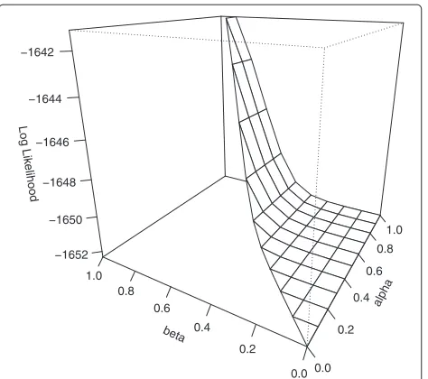
By executing the above command, the maximum likeli-hood estimates were obtained as 0.970, 0.943, and 0.188 with log likelihood value -1640.339. It is important to check whether the iteration converges to the global
max-imum. To this end, we use the PerspPenetrance
function, which draws a perspective plot of the log like-lihood surface fixed on one of the parameters. A plot of the evaluated likelihood for fixed γ = 0.188 is shown in Figure 1. The plot is generated from the following command:
> PerspPenetrance(polynomial, "gamma", 0.188, theta=-60, phi=20)
alpha
0.0 0.2
0.4 0.6
0.8 1.0
beta
0.0 0.2 0.4 0.6 0.8 1.0
Log Lik
elihood
[image:4.595.57.294.85.295.2]−1652 −1650 −1648 −1646 −1644 −1642
Figure 1Perspective plot of the log likelihood surface of the simulation pedigree data withγ=0.188.The simulated pedigree dataset is generated assuming penetrance values 0.95, 0.7, and 0, and disease allele frequency 0.0001. The likelihood of the simulated pedigree data is evaluated with frequency assigned to 0.0001, and the penetrances are estimated by the MLEP package. Fixingγat its estimate 0.188, the log likelihood surface is drawn on a limited region reflecting the parameter constraintα≥β. The maximum appears near those of the other two maximum likelihood estimates (α,β)=(0.970, 0.943).
linear inequality constraints and the initial value ofγ to 0≤γ ≤0.01 and 0.001 as follows:
> constrOptim(c(0.9,0.8,0.001), fr, grr, ui=rbind(c(1,0,0),c(0,1,0),c(0,0,1),
c(-1,0,0),c(0,-1,0),c(0,0,-1), c(1,-1,0),c(0,1,-1)),
ci=c(rep(0,3), rep(-1,2), -0.01, rep(0,2)), poly=polynomial,
control=list(fnscale=-1), mu=0.01)
Following this adjustment, the obtained maximum like-lihood estimates were 0.875, 0.759, and 0.003 with log likelihood value -1644.840 less that of global maximum. The perspective plot for fixed γ = 0.003 is shown in Figure 2 and the maximum is found near those of the other two estimates although the surface is flat around the maximum.
Power Comparison
To assess linkage analysis efficacy for different pene-trance values, the expected LOD score was evaluated by the SLINK package given the following four pene-trance models: true penepene-trance model (0.950, 0.700, and 0.000), dominant model (0.999, 0.999, and 0.000), MLE
alpha
0.0 0.2
0.4 0.6
0.8 1.0
beta
0.0 0.2 0.4 0.6 0.8 1.0
Log Lik
elihood
−4000 −3500 −3000 −2500 −2000
Figure 2Perspective plot of the log likelihood surface of the simulation pedigree data withγ=0.003.The same likelihood polynomial as that of Figure 1 is plotted with theγpenetrance estimate fixed at 0.003. The penetrance estimates are evaluated employing a parameter constraint 0≤γ≤0.01. The maximum appears near those of the other two estimates(α,β)=(0.875, 0.759).
with theγ constraint model (0.875, 0.759, and 0.003), and unrestrained MLE model (0.970, 0.943, and 0.188). The results are summarized in Table 1. In the true penetrance model, the highest LOD score (exceeding 3) is correctly obtained atθ = 0. The dominant model, which is often used for simplicity in practical analysis, yields the high-est LOD score at θ = 0.1. Therefore, researchers may conclude that the disease locus exists relatively close, but not extremely close to, the employed marker. This exam-ple highlights the potential of intuitive approaches to yield an incorrect result. Analysis via MLE constrained by the
γ parameter yields results that match the true model, but unconstrained MLE leads to the uncertain conclusion that the disease locus may not exist near the employed marker, since the maximum LOD score atθ =0.05 in this case is less than 3.
Effect of misspecifying disease allele frequency
[image:4.595.307.539.86.297.2]Table 1 Summary of LOD scores for the four parameter models
Model Recombination fraction (θ)
0 0.05 0.1 0.15 0.2 0.25 0.3 0.35 0.4 0.45
True 4.071 3.831 3.535 3.201 2.835 2.438 2.011 1.553 1.066 0.549
Dominant -0.158 3.296 3.394 3.240 2.965 2.609 2.189 1.714 1.189 0.617
MLE (withγconstraint) 3.992 3.797 3.520 3.198 2.838 2.444 2.017 1.559 1.069 0.550
MLE (unconstrained) 0.781 0.792 0.710 0.603 0.487 0.370 0.260 0.167 0.095 0.041
Data Simulation
The pedigree structure, number of marker alleles, marker allele frequencies, penetrance parameters, and recombi-nation fractions were identical to those used in the previ-ous simulation, while disease allele frequency was altered to 0.0001, 0.001, 0.01, 0.1, or 0.2. 50 pedigree datasets were generated for each disease allele frequency. For the simulated pedigree datasets, disease allele frequency was then assumed to be 0.0001, 0.001, 0.01, 0.1, 0.25, or 0.5, and the likelihood polynomials were evaluated in each case.
Maximum likelihood estimate
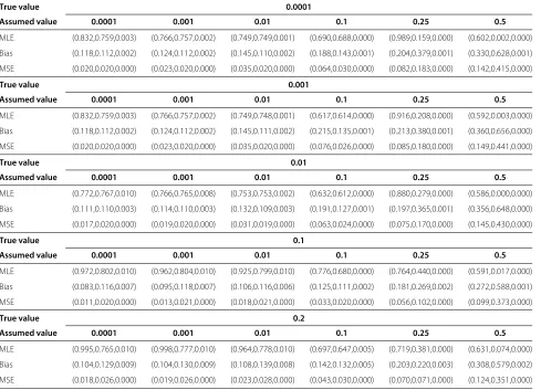
For each of the evaluated likelihood polynomials, we also evaluated their maximum likelihood estimates subject to the constraint 0 ≤ γ ≤ 0.01. The unconstrained esti-mates for disease allele frequency 0.0001 displayed similar bias to the assumed frequency in the previous simula-tion study. Hence we employed the same parameter con-straints as previously applied for all cases in the present simulation, although the constraint exerted little effect on the likelihood estimates at disease allele frequencies greater than 0.0001. The evaluated maximum likelihood
Table 2 Summary of maximum likelihood estimates of penetrance parameters
True value 0.0001
Assumed value 0.0001 0.001 0.01 0.1 0.25 0.5
MLE (0.832,0.759,0.003) (0.766,0.757,0.002) (0.749,0.749,0.001) (0.690,0.688,0.000) (0.989,0.159,0.000) (0.602,0.002,0.000)
Bias (0.118,0.112,0.002) (0.124,0.112,0.002) (0.145,0.110,0.002) (0.188,0.143,0.001) (0.204,0.379,0.001) (0.330,0.628,0.001)
MSE (0.020,0.020,0.000) (0.023,0.020,0.000) (0.035,0.020,0.000) (0.064,0.030,0.000) (0.082,0.183,0.000) (0.142,0.415,0.000)
True value 0.001
Assumed value 0.0001 0.001 0.01 0.1 0.25 0.5
MLE (0.832,0.759,0.003) (0.766,0.757,0.002) (0.749,0.748,0.001) (0.617,0.614,0.000) (0.916,0.208,0.000) (0.592,0.003,0.000)
Bias (0.118,0.112,0.002) (0.124,0.112,0.002) (0.145,0.111,0.002) (0.215,0.135,0.001) (0.213,0.380,0.001) (0.360,0.656,0.000)
MSE (0.020,0.020,0.000) (0.023,0.020,0.000) (0.035,0.020,0.000) (0.076,0.026,0.000) (0.085,0.180,0.000) (0.149,0.441,0.000)
True value 0.01
Assumed value 0.0001 0.001 0.01 0.1 0.25 0.5
MLE (0.772,0.767,0.010) (0.766,0.765,0.008) (0.753,0.753,0.002) (0.632,0.612,0.000) (0.880,0.279,0.000) (0.586,0.000,0.000)
Bias (0.111,0.110,0.003) (0.114,0.110,0.003) (0.132,0.109,0.003) (0.191,0.127,0.001) (0.197,0.365,0.001) (0.356,0.648,0.000)
MSE (0.017,0.020,0.000) (0.019,0.020,0.000) (0.031,0.019,0.000) (0.063,0.024,0.000) (0.075,0.170,0.000) (0.145,0.430,0.000)
True value 0.1
Assumed value 0.0001 0.001 0.01 0.1 0.25 0.5
MLE (0.972,0.802,0.010) (0.962,0.804,0.010) (0.925,0.799,0.010) (0.776,0.680,0.000) (0.764,0.440,0.000) (0.591,0.017,0.000)
Bias (0.083,0.116,0.007) (0.095,0.118,0.007) (0.106,0.116,0.006) (0.125,0.111,0.002) (0.181,0.269,0.002) (0.272,0.588,0.001)
MSE (0.011,0.020,0.000) (0.013,0.021,0.000) (0.018,0.021,0.000) (0.033,0.020,0.000) (0.056,0.102,0.000) (0.099,0.373,0.000)
True value 0.2
Assumed value 0.0001 0.001 0.01 0.1 0.25 0.5
MLE (0.995,0.765,0.010) (0.998,0.777,0.010) (0.964,0.778,0.010) (0.697,0.647,0.005) (0.719,0.381,0.000) (0.631,0.074,0.000)
Bias (0.104,0.129,0.009) (0.104,0.130,0.009) (0.108,0.139,0.008) (0.142,0.132,0.005) (0.203,0.220,0.003) (0.308,0.579,0.002)
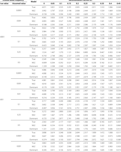
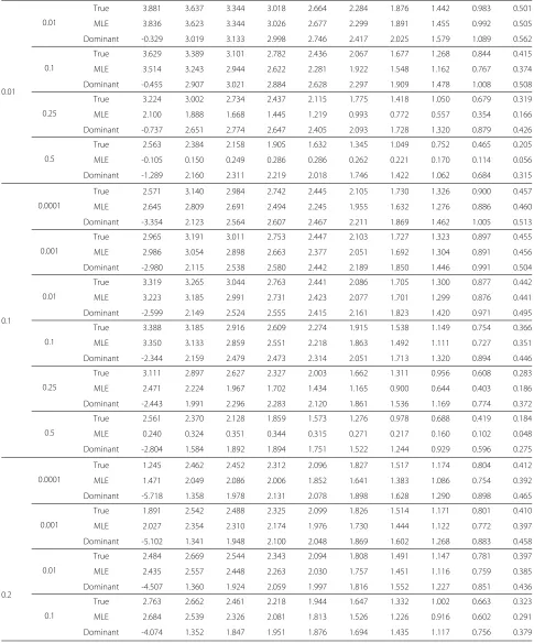
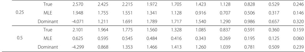
[image:5.595.58.547.382.735.2]Table 3 Summary of LOD scores for the three penetrance models
Disease allele frequency
Model Recombination fraction (θ)
True value Assumed value 0 0.05 0.1 0.15 0.2 0.25 0.3 0.35 0.4 0.45
0.0001
0.0001
True 4.071 3.831 3.535 3.201 2.835 2.438 2.011 1.553 1.066 0.549
MLE 3.992 3.797 3.520 3.198 2.838 2.444 2.017 1.559 1.069 0.550
Dominant -0.158 3.296 3.394 3.240 2.965 2.609 2.189 1.714 1.189 0.617
0.001
True 4.065 3.826 3.530 3.196 2.830 2.434 2.007 1.550 1.063 0.547
MLE 4.003 3.805 3.527 3.204 2.843 2.448 2.021 1.561 1.071 0.550
Dominant -0.188 3.265 3.364 3.211 2.939 2.586 2.170 1.698 1.176 0.609
0.01
True 4.022 3.784 3.489 3.157 2.792 2.398 1.974 1.521 1.040 0.532
MLE 3.984 3.780 3.500 3.175 2.815 2.421 1.995 1.538 1.051 0.538
Dominant -0.234 3.217 3.320 3.171 2.902 2.552 2.138 1.670 1.155 0.598
0.1
True 3.702 3.474 3.191 2.872 2.524 2.150 1.750 1.328 0.887 0.437
MLE 3.665 3.429 3.143 2.823 2.476 2.103 1.708 1.292 0.860 0.422
Dominant -0.425 3.040 3.146 3.002 2.738 2.397 1.997 1.549 1.059 0.534
0.25
True 3.257 3.049 2.787 2.492 2.171 1.827 1.464 1.087 0.704 0.331
MLE 1.524 1.407 1.270 1.121 0.964 0.800 0.634 0.467 0.303 0.146
Dominant -0.743 2.748 2.862 2.727 2.478 2.158 1.783 1.362 0.906 0.437
0.5
True 2.549 2.384 2.165 1.917 1.646 1.359 1.061 0.760 0.469 0.205
MLE -0.009 0.204 0.292 0.321 0.315 0.284 0.238 0.182 0.121 0.059
Dominant -1.339 2.208 2.349 2.250 2.044 1.765 1.434 1.067 0.682 0.311
0.001
0.0001
True 4.086 3.846 3.548 3.213 2.846 2.447 2.019 1.560 1.070 0.551
MLE 4.008 3.812 3.534 3.210 2.849 2.453 2.025 1.565 1.073 0.552
Dominant -0.140 3.312 3.409 3.253 2.977 2.619 2.198 1.721 1.193 0.619
0.001
True 4.081 3.841 3.543 3.208 2.841 2.443 2.014 1.556 1.067 0.549
MLE 4.018 3.820 3.541 3.216 2.854 2.458 2.028 1.567 1.075 0.553
Dominant -0.170 3.281 3.379 3.225 2.951 2.597 2.179 1.705 1.180 0.611
0.01
True 4.038 3.799 3.502 3.169 2.803 2.407 1.981 1.527 1.044 0.534
MLE 4.000 3.795 3.513 3.187 2.825 2.429 2.002 1.543 1.055 0.540
Dominant -0.216 3.234 3.335 3.185 2.915 2.563 2.147 1.677 1.160 0.601
0.1
True 3.717 3.489 3.204 2.884 2.535 2.159 1.757 1.334 0.891 0.439
MLE 3.602 3.338 3.040 2.717 2.372 2.006 1.621 1.221 0.809 0.394
Dominant -0.407 3.056 3.161 3.016 2.751 2.407 2.006 1.556 1.064 0.536
0.25
True 3.272 3.063 2.800 2.503 2.181 1.836 1.471 1.093 0.708 0.332
MLE 1.847 1.667 1.479 1.286 1.090 0.893 0.698 0.508 0.325 0.154
Dominant -0.725 2.765 2.877 2.741 2.490 2.168 1.792 1.369 0.911 0.439
0.5
True 2.563 2.397 2.177 1.927 1.655 1.366 1.067 0.765 0.471 0.207
MLE 0.048 0.234 0.310 0.332 0.321 0.288 0.240 0.183 0.121 0.060
Dominant -1.321 2.225 2.364 2.264 2.056 1.776 1.443 1.073 0.686 0.312
0.0001
True 3.808 3.619 3.348 3.038 2.694 2.317 1.909 1.472 1.008 0.517
MLE 3.647 3.461 3.206 2.913 2.588 2.231 1.841 1.421 0.973 0.499
Dominant -0.374 3.002 3.150 3.037 2.794 2.466 2.072 1.621 1.122 0.580
0.001
True 3.863 3.639 3.355 3.038 2.691 2.313 1.905 1.469 1.005 0.515
MLE 3.730 3.532 3.267 2.964 2.628 2.262 1.864 1.437 0.983 0.503
Table 3 Summary of LOD scores for the three penetrance modelsContinued
0.01
0.01
True 3.881 3.637 3.344 3.018 2.664 2.284 1.876 1.442 0.983 0.501
MLE 3.836 3.623 3.344 3.026 2.677 2.299 1.891 1.455 0.992 0.505
Dominant -0.329 3.019 3.133 2.998 2.746 2.417 2.025 1.579 1.089 0.562
0.1
True 3.629 3.389 3.101 2.782 2.436 2.067 1.677 1.268 0.844 0.415
MLE 3.514 3.243 2.944 2.622 2.281 1.922 1.548 1.162 0.767 0.374
Dominant -0.455 2.907 3.021 2.884 2.628 2.297 1.909 1.478 1.008 0.508
0.25
True 3.224 3.002 2.734 2.437 2.115 1.775 1.418 1.050 0.679 0.319
MLE 2.100 1.888 1.668 1.445 1.219 0.993 0.772 0.557 0.354 0.166
Dominant -0.737 2.651 2.774 2.647 2.405 2.093 1.728 1.320 0.879 0.426
0.5
True 2.563 2.384 2.158 1.905 1.632 1.345 1.049 0.752 0.465 0.205
MLE -0.105 0.150 0.249 0.286 0.286 0.262 0.221 0.170 0.114 0.056
Dominant -1.289 2.160 2.311 2.219 2.018 1.746 1.422 1.062 0.684 0.315
0.1
0.0001
True 2.571 3.140 2.984 2.742 2.445 2.105 1.730 1.326 0.900 0.457
MLE 2.645 2.809 2.691 2.494 2.245 1.955 1.632 1.276 0.886 0.460
Dominant -3.354 2.123 2.564 2.607 2.467 2.211 1.869 1.462 1.005 0.513
0.001
True 2.965 3.191 3.011 2.753 2.447 2.103 1.727 1.323 0.897 0.455
MLE 2.986 3.054 2.898 2.663 2.377 2.051 1.692 1.304 0.891 0.456
Dominant -2.980 2.115 2.538 2.580 2.442 2.189 1.850 1.446 0.991 0.504
0.01
True 3.319 3.265 3.044 2.763 2.441 2.086 1.705 1.300 0.877 0.442
MLE 3.223 3.185 2.991 2.731 2.423 2.077 1.701 1.299 0.876 0.441
Dominant -2.599 2.149 2.524 2.555 2.415 2.161 1.823 1.420 0.971 0.495
0.1
True 3.388 3.185 2.916 2.609 2.274 1.915 1.538 1.149 0.754 0.366
MLE 3.350 3.133 2.859 2.551 2.218 1.863 1.492 1.111 0.727 0.351
Dominant -2.344 2.159 2.479 2.473 2.314 2.051 1.713 1.320 0.894 0.446
0.25
True 3.111 2.897 2.627 2.327 2.003 1.662 1.311 0.956 0.608 0.283
MLE 2.471 2.224 1.967 1.702 1.434 1.165 0.900 0.644 0.403 0.186
Dominant -2.443 1.991 2.296 2.283 2.120 1.861 1.536 1.169 0.774 0.372
0.5
True 2.561 2.370 2.128 1.859 1.573 1.276 0.978 0.688 0.419 0.184
MLE 0.240 0.324 0.351 0.344 0.315 0.271 0.217 0.160 0.102 0.048
Dominant -2.804 1.584 1.892 1.894 1.751 1.522 1.244 0.929 0.596 0.275
0.2
0.0001
True 1.245 2.462 2.452 2.312 2.096 1.827 1.517 1.174 0.804 0.412
MLE 1.471 2.049 2.086 2.006 1.852 1.641 1.383 1.086 0.754 0.392
Dominant -5.718 1.358 1.978 2.131 2.078 1.898 1.628 1.290 0.898 0.465
0.001
True 1.891 2.542 2.488 2.325 2.099 1.826 1.514 1.171 0.801 0.410
MLE 2.027 2.354 2.310 2.174 1.976 1.730 1.444 1.122 0.772 0.397
Dominant -5.102 1.341 1.948 2.100 2.048 1.869 1.602 1.268 0.883 0.458
0.01
True 2.484 2.669 2.544 2.343 2.094 1.808 1.491 1.147 0.781 0.397
MLE 2.435 2.557 2.448 2.263 2.030 1.757 1.451 1.116 0.759 0.385
Dominant -4.507 1.360 1.924 2.059 1.997 1.816 1.552 1.227 0.851 0.436
0.1
True 2.763 2.662 2.461 2.218 1.944 1.647 1.332 1.002 0.663 0.323
MLE 2.684 2.539 2.326 2.081 1.813 1.526 1.226 0.916 0.602 0.291
Table 3 Summary of LOD scores for the three penetrance modelsContinued
0.25
True 2.570 2.425 2.215 1.972 1.705 1.423 1.128 0.828 0.529 0.246
MLE 1.948 1.755 1.551 1.341 1.128 0.916 0.707 0.506 0.317 0.146
Dominant -4.071 1.211 1.691 1.789 1.717 1.540 1.290 0.986 0.657 0.320
0.5
True 2.101 1.964 1.775 1.560 1.328 1.085 0.837 0.591 0.360 0.159
MLE 0.625 0.595 0.545 0.484 0.416 0.343 0.269 0.195 0.125 0.060
Dominant -4.299 0.868 1.353 1.466 1.413 1.260 1.039 0.781 0.509 0.239
estimates, mean absolute bias, and mean squared error (MSE) of the estimates are summarized in Table 2. Note that γ is restricted to small values. When the true fre-quency is 0.0001, 0.001, or 0.01, and the likelihood is also evaluated at one of these frequencies, we find that
α is underestimated andβ is overestimated. If the likeli-hood is evaluated at frequencies exceeding 0.01, the esti-mates become unstable as both the mean bias and MSE become large. Assuming the true frequency to be 0.1 or 0.2 but evaluating the likelihood at frequencies less than 0.1 results in overestimation of bothαandβ. If the likelihood is evaluated at frequency 0.1, the estimates remain biased, but likelihood estimates evaluated at higher allele frequen-cies become unstable. Perspective plots of the resulting log likelihood surfaces at fixedγ are provided as Additional file 2. Although the estimates are biased or unstable, the maxima are correctly located near those of the other two estimates for all cases studied.
Power of detecting linkage
Based on the evaluated maximum likelihood estimates, the expected LOD scores for the following three pene-trance models were evaluated by the SLINK packages; true penetrance model (0.950, 0.700, and 0.000), domi-nant model (0.999, 0.999, and 0.000), and MLE model (the estimates are listed in Table 2). The results are shown in Table 3. The true and MLE models yield maximum LOD scores greater than 3 atθ = 0 when both true and assumed disease allele frequencies are 0.0001, 0.001, or 0.01, or when the true frequency is one of these values and the assumed frequency is 0.1. These models per-formed with similar correctness at true frequency 0.1 and assumed frequency 0.01 or 0.1. The dominant model, on the other hand, yielded poor or misplaced LOD scores for all cases.
These results indicate that genetic diseases with low allele frequencies (<0.01) are suitable for analysis by link-age analysis; that is, the linklink-age between disease locus and marker locus can be correctly identified. At disease allele frequencies exceeding 0.1, the correct conclusion may not be reached because the peak of the significant LOD score (greater than 3) is obtained at different recombination fractions or because the linkage-detecting efficacy is insuf-ficient (i.e., no LOD score higher than 3 is obtained)
even when true penetrance parameters are employed. The MLEP package will almost certainly yield correct results for genetic diseases with small allele frequency, provided that the frequency is also assumed to be 0.1 or less. In this case, incorrectly specifying the disease allele frequency will have little effect on the results. When the true fre-quency is 0.1, assigning a small frefre-quency (of order 0.01) to likelihood evaluations will again yield the correct result. In all other cases, the effect of allele frequency misspeci-fication cannot be neglected. These results were validated by another simulation study, in which true penetrance parameters were assumed to be 0.990, 0.900, and 0.000. Maximum likelihood estimates, LOD scores for the three penetrance models, and perspective plots are provided as Additional files 3, 4, and 5, respectively.
Discussion
We have developed the MLEP R package to explore maximum likelihood estimates of penetrance parameters. The polynomial form of the likelihood evaluation enables flexible exploration of penetrance estimates by evaluat-ing both the likelihood value and its gradient precisely, and by introducing parameter constraints if these can be assumed. Introduction of a low phenocopy rate (γ <0.01) especially improved the quality of the analysis result in the presented simulation study. Convergence may be ver-ified visually by auxiliary perspective plots. The input pedigree datasets bias the evaluated maximum likelihood estimates; however, the likelihood surface may be flat around the maximum and the performance of the esti-mates at correctly identifying linkages is superior to that of intuitive penetrance values.
diseases, are not suitable for analysis by this approach. Disease allele frequency is another unknown important parameter in linkage analysis, but several previous stud-ies have reported that misspecifying the disease allele frequency does not significantly influence to the detec-tion of the linkage [6,17]. Our simuladetec-tion study supports these results, provided that both true and assumed dis-ease allele frequencies are small. It has also been men-tioned that linkage analysis would be successful if a disease allele frequency is rare in the population [18]; therefore, assigning the frequency to a small value for such the disease produces a feasible result. Here, we have demon-strated that linkage analysis using maximum likelihood estimates by the MLEP package correctly localizes a dis-ease locus, if the frequency of the disdis-ease allele is made small (<0.1).
Availability and requirements
• Project name:MLEP
• Project home page:http://cran.r-project.org/web/ packages/MLEP/index.html
http://www.stat.math.keio.ac.jp/∼sugaya/PIA/MLEP/ index.html
• Operating systems:Linux/Mac/Windows • Programming language:R and C • Other requirements:R version≥2.14 • License:GPL≥2
• Any restrictions to use by non-academics:None
Availability of supporting data
The data set supporting the results of this article is available at http://www.stat.math.keio.ac.jp/∼sugaya/PIA/ MLEP/index.html.
Additional files
Additional file 1: Algorithm for likelihood polynomial of penetrance parameters.
Additional file 2: Figure S1.Perspective plots of log likelihood surface for
the simulation study of the penetrance model, 0.950, 0.700, and 0.000. The log likelihood surfaces are plotted for 30 cases of disease allele frequencies of the penetrance model, 0.950, 0.700, and 0.000. Fixingγat its estimate evaluated under the constraint 0≤γ≤0.01, each log likelihood surface is drawn on a limited regionα≥β.
Additional file 3: Table S1.Summary of maximum likelihood estimates
of penetrance parameters for the simulation study of the penetrance model, 0.990, 0.900, and 0.000. The pedigree structure, number of marker alleles, marker allele frequencies, and recombination fractions are identical to those used in the simulation for the penetrance model, 0.950, 0.700, and 0.000, while penetrance parameters are assumed to be 0.990, 0.900, and 0.000. Six pedigree datasets with 50 pedigrees are generated, assuming disease allele frequencies to be 0.0001, 0.001, 0.01, 0.1, and 0.2. For each datasets, the likelihood polynomial is evaluated, assuming the frequency to be 0.0001, 0.001, 0.01, 0.1, 0.25, and 0.5, and the maximum likelihood estimates are evaluated under the constraint 0≤γ≤0.01.
Additional file 4: Table S2.Summary of LOD scores for the simulation
study of the penetrance model, 0.990, 0.900, and 0.000. LOD scores are evaluated for 30 cases of disease allele frequencies for three penetrance models; true penetrance model (0.990, 0.900, and 0.000), dominant model (0.999, 0.999, and 0.000),and MLE model (the estimates are listed in Supplementary Table S1).
Additional file 5: Figure S2.Perspective plots of log likelihood surface for
the simulation study of the penetrance model, 0.990, 0.900, and 0.000. The log likelihood surfaces are plotted for 30 cases of disease allele frequencies of the penetrance model, 0.990, 0.900, and 0.000. Fixingγat its constrained estimate under the 0≤γ≤0.01, each log likelihood surface is drawn on a limited regionα≥β.
Competing interests
The author declares no competing interests.
Author’s contributions
YS implemented the software and prepared the manuscript.
Acknowledgements
The author is grateful to Professor Ritei Shibata at Keio University for his helpful suggestions. The author thanks the anonymous referees for their careful reading of the manuscript and their valuable comments and suggestions.
Received: 11 February 2012 Accepted: 21 August 2012 Published: 28 August 2012
References
1. Morton NE:Sequential tests for the detection of linkage.Am J Hum Genet1955,7:277–318.
2. Mattheisen M, Dietter J, Knapp M, Baur MP, Strauch K:Inferential testing for linkage with GENEHUNTER-MODSCORE: the impact of the pedigree structure on the null distribution of multipoint MOD
scores.Genet Epidemiol2008,32:73–83.
3. Dietter J, Mattheisen M, F ¨urst R, R ¨uschendorf F, Wienker TF, Strauch K: Linkage analysis using sex-specific recombination fractions with
GENEHUNTER-MODSCORE.Bioinformatics2007,23:64–70.
4. Strauch K, F ¨urst R, R ¨uschendorf F, Windemuth C, Dietter J, Flaquer A, Baur MP, Wienker TF:Linkage analysis of alcohol dependence using MOD
scores.BMC Genetics2005,6(Suppl1):S162.
5. Strauch K:Parametric linkage analysis with automatic optimization
of the disease model parameters.Am J Hum Genet2003,
73(Suppl1):A2624.
6. Clerget-Darpoux F, Bona¨ıti-Pelli`e C, Hochez J:Effects of misspecifying
genetic parameters in lod score analysis.Biometrics1986,
42(2):393–399.
7. Wang Y, Ottman R, Rabinowitz D:A method for estimating penetrance
from families sampled for linkage analysis.Biometrics2006,
62:1081–1088.
8. Swartz MD, Minard CG, Amos CI:The relative efficiency of penetrance
estimators for sib pairs.Hum Hered2005,59:61–66.
9. Maplesoft, a division of Waterloo Maple Inc.:Maple V. Version release 5.1. Ontario, Canada; 1999 .
10. Maplesoft, a division of Waterloo Maple Inc.:Maple 6. Ontario, Canada; 2000.
11. R Development Core Team:R: A Language and Environment for Statistical Computing.R Foundation for Statistical Computing. Vienna, Austria; 2011. [http://www.R-project.org/] [ISBN 3-900051-07-0]
12. Sugaya Y, Shibata R:Exploration of the disease locus by a careful
evaluation of the likelihood polynomial for pedigree data.J Hum
Genet2011,56:383–389.
13. Ott J:Computer-simulation methods in human linkage analysis.Proc Natl Acad Sci USA1989,86:4175–4178.
14. Weeks DE, Ott J, Lathrop GM:SLINK: a general simulation program for
linkage analysis.Am J Hum Genet1990,47:A204.
15. Kamatani N, Moritani M, Yamanaka H, Takeuchi F, Hosoya T, Itakura M: Localization of a gene for familial juvenile hyperuricemic nephropathy causing underexcretion-type gout to 16p12 by
genome-wide linkage analysis of a large family.Arthritis Rheum2000,
16. Lange K:Numerical Analysis for Statisticians. New York: Springer; 1999. 17. Pal DK, Durner M, Greenberg DA:Effect of misspecification of gene
frequency on the two-point LOD score.Eur J Hum Genet2001,
9:855–859.
18. Bailey-Wilson JE, Wilson AF:Linkage analysis in the next-generation
sequencing era.Hum Hered2011,72(4):228–236.
doi:10.1186/1756-0500-5-465
Cite this article as:Sugaya:MLEP: an R package for exploring the maximum likelihood estimates of penetrance parameters.BMC Research Notes2012 5:465.
Submit your next manuscript to BioMed Central and take full advantage of:
• Convenient online submission
• Thorough peer review
• No space constraints or color figure charges
• Immediate publication on acceptance
• Inclusion in PubMed, CAS, Scopus and Google Scholar
• Research which is freely available for redistribution