This is a repository copy of
Design and validation of an unmanned surface vehicle
simulation mode
.
White Rose Research Online URL for this paper:
http://eprints.whiterose.ac.uk/112449/
Version: Accepted Version
Article:
Heins, P.H., Jones, B. orcid.org/0000-0002-7465-1389 and Taunton, D.J. (2017) Design
and validation of an unmanned surface vehicle simulation mode. Applied Mathematical
Modelling. ISSN 0307-904X
https://doi.org/10.1016/j.apm.2017.02.028
Reuse
This article is distributed under the terms of the Creative Commons Attribution-NonCommercial-NoDerivs (CC BY-NC-ND) licence. This licence only allows you to download this work and share it with others as long as you credit the authors, but you can’t change the article in any way or use it commercially. More
information and the full terms of the licence here: https://creativecommons.org/licenses/
Takedown
If you consider content in White Rose Research Online to be in breach of UK law, please notify us by
Design and validation of an unmanned surface vehicle
simulation model
Peter H. Heinsa,∗, Bryn Ll. Jonesa, Dominic J. Tauntonb
a
Department of Automatic Control and Systems Engineering, The University of Sheffield, Sheffield, U.K.
b
Engineering and the Environment, University of Southampton, Southampton, U.K.
Abstract
In this paper we present a multiphysics simulation model of Halcyon, an autonomous unmanned surface vehicle (USV). The simulation model presented in this paper has been developed to rapidly progress the design, development and validation of Halcyon’s autonomy management system, par-ticularly in challenging sea conditions. Using simulation for this purpose enables extensive testing across the full environmental operating envelope of the vessel, hence greatly reducing the need for real-world sea-trials. The simulator is comprised of a novel and comprehensive sea-surface wave environment model, a six degree of freedom nonlinear unified seakeeping and manoeuvring boat dynamics model, an actuation dynamics model, an autopilot and an interface with an autonomy management system. Results are presented that show good agreement between real-world and simulated sea-trials data.
Keywords: multiphysics, ship modelling, wave modelling, simulation, model validation
1. Introduction
Unmanned surface vehicles (USVs) are autonomous marine craft that operate on the surface of a body of water without any personnel onboard. They are analogous to airborne unmanned aerial vehicles (UAVs) and subaquatic unmanned underwater vehicles (UUVs) [1]. USVs have been widely used to conduct scientific research in the fields of oceanography [2] and meteorology [3] and have their applications in the oil and gas industry also. Within the Defence sector, USVs are currently being developed for several roles including anti-submarine warfare and minesweeping. One such USV isHalcyonwhich is currently being developed by Thales UK and ASV Global for autonomous mine clearing missions. The simulation model presented in this paper has been developed to aid in the development, testing and validation of Halcyon’s autonomy management system. Using simulation for this purpose reduces the need to conduct time-consuming and expensive sea-trials and allows for greater flexibility over the environmental conditions in which the boat must operate. This flexibility offers the additional advantage of being able to test and evaluate several guidance, navigation and control (GNC) systems using the same “random” wave environment. To aid in this, the simulator incorporates a novel sea-surface wave environment model which is an integration of
∗Corresponding author
Figure 1: Drawings of Halcyon.
several spectral wave models and is capable of simulating omnidirectional surface waves produced or affected by ocean swell, local wind, surface currents and finite water depth.
Drawings of Halcyon are shown in Figure 1 and a brief technical specification is given in Table 1. The craft’s hydrodynamic parameters, which determine the various forces imparted upon the vessel from the surrounding water, depend heavily on the geometry of the hull and the boat’s mass distribution. In the current work, these are calculated using the hydrodynamic code THARBM [4]. Model parameters that are unknown a priori are identified by comparing simulation output to sea-trials data for Halcyon.
The overarching objective of the simulation model is to provide a physics-based platform for rapidly developing and evaluating a USV’s autonomy management system. This means that in designing the simulation model, a compromise must be struck between the efficiency of evaluation, in order that simulations can be ran in real-time, and the accuracy of the solution. With this in mind, the simulation model need only retain the key physics sufficient to achieve good qualitative agreement with the sea-trials data.
Modern USVs vary in their shape, size and configuration. Smaller USVs which are O(10−1
)-O(100) metres in length, tend to be deployed mainly for scientific research [5] as well as for security monitoring [6]. Larger USVs which areO(101) metres in length are used in a wider variety of roles including Defence-based roles. Halcyon, beingO(101) metres in length and having a “patrol boat” hull form, is representative of a wide array of medium-to-large sized USVs which are currently being developed by the Defence industry. Therefore, given a full set of rigid body and hydrodynamic data, the model presented in the following could be quickly parameterised to simulate the dynamics of many current or future USVs.
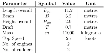
Parameter Symbol Value Unit
Length overall Loa 11.2 metres
Beam B 3.2 metres
Height overall Hoa 2.9 metres
Draft T 0.7 metres
Mass m 11000 kilograms
Top Speed 25 knots
No. of engines 2
[image:4.612.197.417.93.206.2]No. of rudders 2
Table 1: Halcyon’s technical specifications.
to marine craft navigating in calm waters. The USV simulation model outlined in this paper rigorously accounts for wind and wave-induced forces and is therefore applicable to a wider range of sea conditions.
The remainder of this paper is organised as follows. An overview of the simulation model and its major components is given in Section 2, the novel wave environment model is presented in Section 3, the reference frames used to derive the simulation model are outlined in Section 4, the six degree of freedom rigid body dynamics model is presented in Section 5, Section 6 outlines the actuation dynamics model, the autopilot and autonomy management system interface are discussed in Section 7, Section 8 presents the sea-trials validation and model tuning exercise, and finally concluding remarks are given in Section 9.
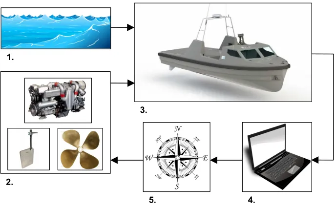
2. Overview of the simulation model
The simulation model consists of five major components: a six degree of freedom boat dynamics model, an actuation dynamics model, a wave environment model, an interface with the autonomy management system and an autopilot. These are illustrated in Figure 2.
A six degree of freedom nonlinear unified seakeeping and manoeuvring model with fluid mem-ory effects [12] is used to model the inertial motions of Halcyon. Speed-dependent damping and hydrodynamic added-mass are included in this model. Wave-induced forces are modelled as a set of speed-dependent response amplitude operator (RAO) data which have been calculated using a hydrodynamic code based upon the hull geometry. Models for Halcyon’s rudders, propellers and engines have also been developed to accurately simulate the vessel’s actuation dynamics.
Besides the boat dynamics model, a multiphysics wave environment model has been developed to simulate dynamic environmental disturbances. This model generates omnidirectional surface waves produced from the combined effects of gusting local wind, ocean swell, surface current and finite water depth. This is achieved by integrating several semi-empirical spectral models.
1.
2.
5. 4.
[image:5.612.135.478.93.307.2]3.
Figure 2: A diagram showing the interactions between the simulation model’s components: 1. Wave environment model, 2. Actuation dynamics model, 3. Boat dynamics model, 4. Autonomy management system interface, 5. Autopilot.
thrust and rudder settings based on the desired speed and heading information sent by MOOS-IvP. The autopilot consists of three proportional-integral-differential (PID) controllers which have been tuned specifically for Halcyon.
3. Wave Environment Model
Relatively lightweight vessels, such as Halcyon, experience significant perturbations in all six degrees of freedom due to the hydrodynamic forces imparted from the surrounding waves. It is therefore imperative that surface waves and their interactions with a moving vessel are modelled appropriately.
The first-order wave-induced forces experienced by a vessel,τwave∈R6, are calculated as [14]:
τwave{dof}= N
X
i=1 M
X
j=1
ρwg
F
{dof}
wave (U, ki, θj)
Aki,θjcos
ωe(U, ki, θj)t+∠Fwave{dof}(ki, θj) +ǫki
, (1)
where dof∈ {1,2,3,4,5,6},ρw= 1025 kg/m3 is the density of seawater,g= 9.81 m/s2is accelera-tion due to gravity,Fwave ∈C6are complex-valued normalised force response amplitude operators (RAOs) and Aki,θj ∈Ris the amplitude of a wave with spatial wavenumberki ∈Rand direction
θj∈R. Lastly,ǫki∈[0,2π] is a random added phase component, and encounter frequency,ωe∈R,
is defined:
ωe(U, ki, θj) :=ωi−
ω2
i
g Ucos(θj), (2)
whereU ∈Rdenotes forward speed, angular frequency is defined via the linear dispersion relation
asω2
Swell
EY Spectrum
Local Wind
TMA Spectrum
M
Ψ
EYΨ
TMACurrent
Nwogu Spectrum
Ψ
TotalΨ
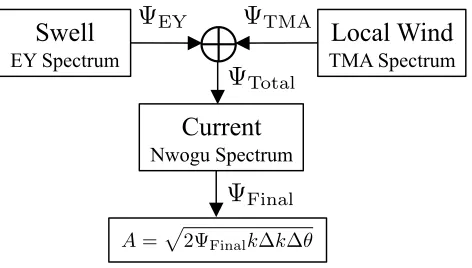
Final [image:6.612.190.426.93.227.2]A=p2ΨFinalk∆k∆θ
Figure 3: Schematic of how wave amplitudes are generated in the wave environment model.
The wave environment model computes the wave amplitudes, Aki,θj, from a combination of
spectral wave models (SWMs) which model the effects of ocean swell, local wind, surface current and finite water depth. For a given set of inputs such as, for instance, water depth and windspeed, each SWM produces a continuous omnidirectional wave energy spectrum (k, ✓) ∈ R. In the
wave environment model, Elfouhaily (EY) [16] and Texel-MARSEN-ARSLOE (TMA) [17] spectra are superimposed to produce a total continuous wave energy spectrum: Total = EY+ TMA. This is analogous to the Torsethaugen [18] and Ochi-Hubble [19] multi-peak SWMs which have low-frequency (ocean swell) and high frequency (local wind) spectral peaks. However, neither the Torsethaugen or Ochi-Hubble SWMs include the effects of finite water depth. The total wave energy spectrum is then multiplied by Nwogu’s current influence spectrum [20],C(k, ✓)∈ R, to produce
the final continuous wave energy spectrum:
Final(k, ✓) =C(k, ✓)◦ Total(k, ✓), (3)
where ◦ denotes a Hadamard dot product. The discrete wave amplitudes are calculated from (3) as:
Aki,θj = q
2 Final(ki, ✓j)ki∆k∆✓, (4)
where ∆k := |ki+1−ki| and ∆✓ := |✓j+1−✓j|. A schematic showing how wave amplitudes are generated is shown in Figure 3.
All omnidirectional SWMs have the form:
(k, ✓) =S(k)D(k, ✓), (5)
whereS(k)∈Ris termed the unidirectional wave spectrum, andD(k, ✓)∈Ris called the spreading
function. S(k) dictates the amount of energy that is contained in the waves’ spatial frequencies, and can be used alone to reconstruct unidirectional surface waves. D(k, ✓) is required to spread the wave energy to waves travelling in directions other than the principle wave direction. The SWMs used in the wave environment model will be outlined in the following sections.
3.1. Elfouhaily (EY) spectrum
ocean surface modelling [21, 22]. For the EY spectrum, S(k) is comprised of a low-frequency wave spectrum, a modified JONSWAP spectrum [23], and a high-frequency wave spectrum. It incorporates a spreading function which ensures long waves are aligned with the principle wind direction and short waves are more directional; something witnessed from radar observations [16]. The EY SWM is given as [16]:
EY(k, ✓,ΛEY) = 1 2πk
−4[B
l(k,ΛEY) +Bh(k,ΛEY)]DEY(k, ✓,ΛEY), (6)
where parameter vector ΛEY=
Us xf βs
⊤
,Usis swell windspeed 10 metres above sea level,
xF is fetch in metres andβsis the principle swell direction. The low-frequency spectral components are modelled as:
Bl(k,ΛEY) = 1 2αp
cp
cFp, (7)
where,
αp= 6×10⁻³
√
Ω, Ω =Us/cp= 0.84 tanh
n
(X/X0)0.4
o−0.75 ,
cp=c(kp), kp=k0Ω2, k0=g/Us2,
c=ω/k, X=k0xF, X0= 2.2×10⁴,
Fp=LPMJpexp
(
−√Ω 10
"s k
kp −
1
#)
, LPM= exp
−54(kp/k)2
,
Jp=γΓ, Γ = exp
− q k kp −1
2
2σ2
, σ= 0.08
1 + 4Ω−3 ,
γ=
(
1.7 0.84<Ω<1 1.7 + 6 log(Ω) 1<Ω<5 ,
Ω is dimensionless inverse wave age andc is wave phase speed. The high-frequency spectral components are modelled as:
Bh(k,ΛEY) =
1 2αm
cm
c Fm, (8)
where,
αm= 10−2
(
1 + ln(u∗/c
m) foru∗< cm
1 + 3 ln(u∗/c
m) foru∗> cm
, cm=c(km) = 0.23m/s,
u∗=pCDNUs, CDN = 5.1×10⁻⁴Us0.46,
Fm= exp
(
−1 4
k
km −
1
kx
-1 -0.5 0 0.5 1
ky -1 -0.8 -0.6 -0.4 -0.2 0 0.2 0.4 0.6 0.8 1 -7 -6 -5 -4 -3 -2 -1 0 1 (a) kx
-1 -0.5 0 0.5 1
[image:8.612.119.489.106.258.2]ky -1 -0.8 -0.6 -0.4 -0.2 0 0.2 0.4 0.6 0.8 1 -7 -6 -5 -4 -3 -2 -1 0 1 (b)
Figure 4: Contour plots of: (a) log10ΨEY(kx =kcos(θ), ky =ksin(θ)) for southerly swell windspeed 10m/s, 104 km fetch, Sea State 4 and (b) log10ΨEYˆ for northerly surface current speedUc= 2m/s, southerly swell windspeed 10m/s, 104km fetch and corresponding to Sea State 5.
andu∗ is the friction velocity at the water surface.
The spreading function used in the EY SWM is given as:
DEY(k, ✓,ΛEY) = [1 + ∆(k) cos(2{✓+βs})]
cos(✓+βs) 2
2
, (9)
where,
∆(k) = tanh
a0+ap(c/cp)2.5+am(cm/c)2.5 ,
a0=
ln(2)
2 , ap= 4, am= 0.13
u∗
cm
.
An example EY spectrum is plotted in Figure 4(a). It can be seen that the EY spectrum is highly directional with a significant portion of energy given to waves travelling in directions far from the principle wind direction. Note that in the plot,kx=kcos(✓) is a North-facing wavenumber vector andky =ksin(✓) is an East-facing wavenumber vector. Figure 5(a) is a sea-surface elevation (η) plot produced using the spectrum shown in Figure 4(a). The high directionality of the waves are easier to visualise in this plot.
Note that in Figures 5(a), 5(b) and 7 a large number of waves are used to produce the sea-surface elevation plots. This is for illustrative purposes only. The number of individual waves that are included in the USV simulation model is typically much smaller. For instance, the number of waves that were included in the simulations presented in Section 8 was 322. This was enough to capture the non-negligible wave-induced forces.
3.2. Texel-MARSEN-ARSLOE (TMA) spectrum
(a) (b)
Figure 5: Sea-surface elevation plots of: (a) ocean swell produced using the EY spectrum in Figure 4(a), (b) ocean swell travelling against a surface current produced using the EY spectrum and current influence spectrum in Figure 4(b). Both plots are comprised of 5122
waves.
of the TMA spectrum decreases with reducing water depth, i.e. the waves have less energy. For deep water,d→ ∞, the TMA spectrum converges to the JONSWAP spectrum. The unidirectional TMA spectrum is [17]:
STMA(k,ΛTMA) =
α
2k
−3φ
PM(ω)φJ(ω), (10)
where parameter vector ΛTMA =
¯
Uw d β¯w
⊤
, ¯Uw is the mean local windspeed 10 metres above sea level,dis the water depth, ¯βwis the mean principle local wind direction,
α= 0.0078κ0.49, κ= U¯w2kp
g , φPM(ω) = exp −
5 4
ω
ωp
−4!
, ωp= 0.2π,
φJ(ω) = exp
h
ln(γ) exp−(ω−ωp)2/2σ2ω2p
i
, γ= 3.3,
σ=
(
0.07 ω≤ωp
0.09 ω > ωp
.
The linear dispersion relation is used to numerically convert peak angular frequency, ωp to peak wavenumber,kp, i.e.:
ω2
p=gkptanh(kpd).
The finite water depth effects are produced via this relation.
[image:9.612.114.498.112.289.2]kx
-1 -0.5 0 0.5 1 ky
-1 -0.8 -0.6 -0.4 -0.2 0 0.2 0.4 0.6 0.8 1
[image:10.612.192.404.103.267.2]-7 -6 -5 -4 -3 -2 -1 0 1
Figure 6: A contour plot of log10ΨTMA(kx =kcos(θ), ky =ksin(θ)) for Southerly mean local windspeed 10m/s, s= 50,d= 20m and corresponding to Sea State 3.
spectrum to model local wind effects, which is given as [24]:
DTMA(✓,ΛTMA) =
2(2s−1)
π
Γ2(s+ 1) Γ(2s+ 1)
cos2s
✓+ ¯β
w 2
, (11)
wheresis called the spreading parameter and Γ(·) denotes the gamma function:
Γ(n) = (n−1)! . (12)
The larger the value of s, the more the waves are aligned with the principle wind direction. It makes physical sense that waves generated by local winds will be closely aligned with the wind direction, therefore a high spreading parameter ofs = 50 is used. An example directional TMA spectrum is plotted in Figure 6. When compared to the EY spectrum plotted in Figure 4(a), the TMA spectrum is shown to be a lot less directional, with the majority of energy allotted to a narrow band of waves closely aligned with the principle wind direction. This can be seen more easily in the sea-surface plot shown in Figure 7 which was produced using the spectrum plotted in Figure 6.
3.3. Nwogu’s current influence spectrum
Surface currents can be produced by various environmental forces such as tide, wind and the Coriolis effect. Currents of sufficient speed can have large effects on surface waves. When waves travel against a current, they increase in amplitude and may eventually break. Waves travelling with a current will reduce in amplitude. Nwogu [20] devised a method for altering a wave energy spectrum to include the effects of a surface current. This is achieved by element-wise multiplying a wave spectrum with no current, Ψ, with a current influence spectrumC(k, ✓). The current influence spectrum is defined as [20]:
C(k, ✓,ΛN) := kCg0
k0(Cg+Uccos✓)
1−Uckcos✓
ω
Figure 7: A sea-surface elevation plot of local wind-driven waves produced using the TMA spectrum plotted in Figure 6 comprised of 5122waves.
where parameter vector ΛN = Uc βc
⊤
, Uc is the surface current speed, βc is the principle current direction,
k0cos ∆✓0,c=kcos ∆✓c, ∆✓0,c=βc−✓0, ∆✓c=βc−✓,
Cg:=∂ω/∂kis the group velocity of the waves relative to the current and variables with subscript 0denote values without the effects of current. The main limitation with the above model is that it produces unrealistically large values for the directional energy spectrum asCg+Uccosθapproaches zero. Waves can no longer penetrate the current when the limitCg=−Uccosθis reached and in reality, would break before reaching that point. The wave environment model neither models nor simulates breaking waves. Therefore, Nwogu’s current influence spectrum is modified in two ways. Firstly, the amplitude of “breaking waves” is set to zero, i.e. C= 0 if Cg ≤ −Uccosθ. Secondly, saturation limits are applied to the higher wavenumbers in the spectrum to prevent unphysical amplitudes of high spatial frequency waves. This is achieved by multiplying the current influence spectrum by k0−5 for wavenumbers k0 > 1. Figure 4(b) shows the effects of current on the EY spectrum shown in Figure 4(a). The current is travelling in the opposite direction to the principle swell wind direction. This has the effect of reducing the directionality of the spectrum and increasing the energy of the higher spatial frequency wave components. This is illustrated more clearly in the surface elevation plot shown in Figure 5(b) which was produced using the spectrum shown in Figure 4(b).
3.4. Variable environment implementation
mean local windspeed ¯Uw, local wind principle directionβw, surface current speedUc, and surface current principle directionβc. These environmental factors vary in the following manner.
For swell windspeed, EY spectra are generated for the initial swell windspeed at time t = Ti and the final swell windspeed at time t = Tf. The implemented spectrum then changes linearly from the initial to the final spectra by means of a gradient matrixGEY:
GEY= EY(k, ✓,ΛEY(Tf))− EY(k, ✓,ΛEY(Ti))
Tf−Ti
,
EY(k, ✓,ΛEY(t)) =
EY(k, ✓,ΛEY(Ti)) t≤Ti
EY(k, ✓,ΛEY(Ti)) +GEY[t−Ti] Ti≤t≤Tf
EY(k, ✓,ΛEY(Tf)) t≥Tf
.
Similarly for mean local windspeed:
GTMA,S= STMA(k,ΛTMA(Tf))−STMA(k,ΛTMA(Ti))
Tf−Ti
,
STMA(k,ΛTMA(t)) =
STMA(k,ΛTMA(Ti)) t≤Ti
STMA(k,ΛTMA(Ti)) +GTMA,S[t−Ti] Ti≤t≤Tf
STMA(k,ΛTMA(Tf)) t≥Tf
,
and local wind principle direction.
GTMA,D=DTMA(✓,ΛTMA(Tf))−DTMA(✓,ΛTMA(Ti))
Tf−Ti
,
DTMA(✓,ΛTMA(t)) =
DTMA(✓,ΛTMA(Ti)) t≤Ti
DTMA(✓,ΛTMA(Ti)) +GTMA,D[t−Ti] Ti≤t≤Tf
DTMA(✓,ΛTMA(Tf)) t≥Tf
.
The current influence spectrum is recalculated every time step of the simulation with linearly varying current speed and current direction:
GC,U= Uc(Tf)−Uc(Ti)
Tf−Ti
, GC,β= βc(Tf)−βc(Ti)
Tf−Ti
,
Uc(t) =
Uc(Ti) t≤Ti
Uc(Ti) +GC,U[t−Ti] Ti ≤t≤Tf
Uc(Tf) t≥Tf
,
βc(t) =
βc(Ti) t≤Ti
βc(Ti) +GC,β[t−Ti] Ti≤t≤Tf
βc(Tf) t≥Tf
3.5. Wind gust modelling
The wave environment model generates a gusting local wind in order to simulate realistic wind-induced forces,τwind, on the vessel. The local windspeedUwis decomposed in the following manner:
Uw(t) = ¯Uw+λgUg(t), (14)
where ¯Uw is the mean windspeed 10 metres above sea level,Ug is the gust component and λg is a gust factor. In a similar fashion to surface waves, several spectral models have been developed for wind gusts. The NPD wind gust spectrum is used which has the form [25]:
SNPD(f) = 320
¯
Uw
10
2
(1 +xn)35n
, x= 172f
¯
Uw
10
−3 4
, (15)
wheren=0.468 andf is frequency in Hertz. The time-varying wind gust component is then calcu-lated from:
Ug(t) = Nf X
i=1
hp
2SNPD(fi)∆fcos (2πfit+φi)
i
, (16)
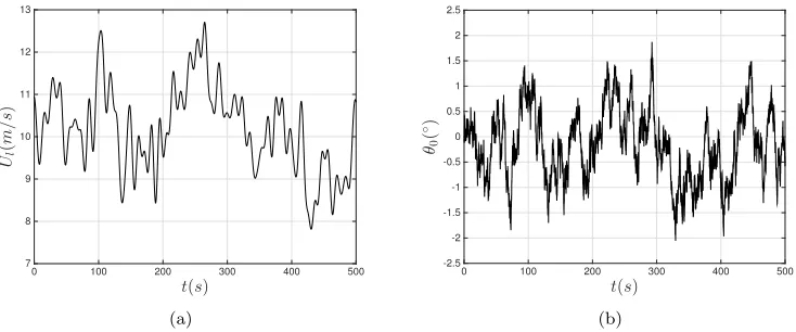
where ∆f =|fi+1−fi| is the sample frequency interval, and φ ∈[0,2π] is random added phase. The wind gust factor λg in (14) can be varied to intensify or attenuate the strength of the gust component. An example plot of the gusting local wind variation is shown in Figure 8(a).
The local wind direction angle,βw, also varies with time. Like for the local windspeed, the wind angle can also be decomposed into a mean component and varying component, i.e. βw= ¯βw+βw′ . The varying component is modelled using a 1st-order Gauss-Markov process [26]:
˙
βw′ +µβw′ =w, (17)
whereµ >0 is a constant fluctuation coefficient andwis white noise. Figure 8(b) shows an example plot of the wind angle variation.
The wind-induced forces experienced by a USV are modelled as [14]:
τwind= 1
2ρaV 2 rw
CX(γrw)AF w
CY(γrw)ALw 0
CK(γrw)ALwHLw 0
CN(γrw)ALwLoa
, (18)
whereρa= 1.225 kg/m3is the density of air,AF wis the frontal exposed projected area of the vessel,
ALw is the lateral exposed projected area of the vessel, HLw is the vertical coordinate above the waterline of the centroid ofALwandLoa is the overall length of the vessel. The relative windspeed and angle are defined respectively:
Vrw=
p u2
rw+v2rw, (19a)
t(s)
0 100 200 300 400 500 Ul ( m/s ) 7 8 9 10 11 12 13 (a)
t(s)
0 100 200 300 400 500
θ0 ( ◦) -2.5 -2 -1.5 -1 -0.5 0 0.5 1 1.5 2 2.5 (b)
Figure 8: (a) An example local windspeed variation with gusting component calculated from the NPD wind gust spectrum, for ¯Uw= 10m/s,λg = 1 andNf = 100. (b) An example local wind angle variation, with fluctuations to the mean calculated using a 1st-order Gauss-Markov process, forµ= 0.1 and ¯β
w= 0.
where
urw=u−uw, vrw=v−vw,
uw=Uwcos(βw−ψ), vw=Uwsin(βw−ψ),
uandvare the surge and sway velocities, andψdenotes the heading angle of the vessel. The atan2 operator is defined as:
atan2(v, u) =
arctan(v
u) ifu >0,
π
2 −arctan( u
v) ifv >0, −π
2 −arctan( u
v) ifv <0, arctan(vu)±π ifx <0,
undefined ifu= 0 andv= 0.
(20)
Returning back to (18),CX(γrw),CY(γrw),CK(γrw) andCN(γrw) denote wind drag coefficients in the surge, sway, roll and yaw degrees of freedom respectively. These coefficients vary with relative wind angle and can be obtained for a specific vessel from scale model testing or via a computational fluid dynamics program. For the current simulation model, the wind coefficients of Blendermann [27] are used. Blendermann performed wind tunnel tests on 17 different types of vessel and derived the following semi-empirical expressions for the coefficients:
CX(γrw) =−CDlAF(γrw)
cos(γrw)
1−δ 2
1−CDl
CDt
sin2(2γrw)
, (21a)
CY(γrw) =CDt
sin(γrw)
1−δ2
1−CDl
CDt
sin2(2γrw)
[image:14.612.122.489.106.259.2]Parameter Symbol Value
Lateral resistance coeff. CDt 0.90
Longitudinal resistance coeff. (head wind) CDlAF(γrw<=π/2) 0.55
Longitudinal resistance coeff. (tail wind) CDlAF(γrw> π/2) 0.60
Cross-force parameter δ 0.60
Rolling moment factor κ 1.1
Frontal projected area AF w 2.4m2
Lateral projected area ALw 16m2
[image:15.612.142.476.94.220.2]Horizontal coordinate of centroid ofALw sL -1.2m Vertical coordinate of centroid ofALw HLw 0.7m
Table 2: Wind-induced force parameters for Halcyon. Parameters 1-5 taken from Blendermann [27] for vessel type: ‘Speed boat’.
CK(γrw) =κCY(γrw), (21c)
CN(γrw) =
sL
Loa −0.18
γrw−π
2
CY(γrw), (21d)
whereCDlAF is the longitudinal resistance coefficient,CDtis the lateral resistance coefficient,δis
the cross-force parameter, κis the rolling moment factor, CDl =CDlAF(γrw)
AF w
ALw and sL is the
horizontal coordinate of the centroid of the transverse projected areaALwwith respect to the main section. The coefficients used for Halcyon are summarised in Table 2.
4. Reference frames
In order to model the rigid body motions of a craft, a number of reference frames must be defined. In modelling Halcyon, two reference frames are used: a body-fixed reference frame which shall be referred to as theb-frame, and a North-East-Down (NED) reference frame which shall be referred to as then-frame.
Theb-frame is fixed to and moves with the vessel and has its origin,Ob, at some fixed location on the vessel. In what follows, this origin is set at the location of Halcyon’s centre of gravity. The co-ordinate system used in theb-frame is illustrated in Figure 9 where it can be seen thatxb lies in the horizontal plane and points from aft to fore,yb lies in the horizontal plane and points from port to starboard, andzb lies in the vertical plane and points downwards. The vessel’s linear and angular velocities are expressed in this reference frame.
Then-frame is fixed to and moves with the earth and has it’s origin,On, at a prescribed location on the earth’s surface. It is defined as a tangent plane on the earth’s surface centred at On and is therefore only applicable for vessels operating in an area close to this origin; otherwise knows as flat earth navigation. Then-frame shall be considered inertial. The co-ordinate system used is illustrated in Figure 9. Axisxn points towards true North, axis yn points towards East, and axis
znpoints down towards the centre of the Earth. Linear and angular positions are expressed in this reference frame.
x
by
bz
bOb
O
nz
n,
D
x
n,
N
[image:16.612.203.415.148.316.2]y
n,
E
Figure 9: A diagram illustrating the body-fixed reference frame with originOb and the North-East-Down (NED) reference frame with originOn.
DOF Description Forces/
moments
Linear/ angular velocities
Position/ Euler angles
1 Linear motion alongx(Surge) X u xn
2 Linear motion alongy (Sway) Y v yn
3 Linear motion alongz (Heave) Z w zn
4 Angular motion aboutx(Roll) K p φ
5 Angular motion abouty (Pitch) M q ✓
6 Angular motion aboutz (Yaw) N r ψ
[image:16.612.122.498.463.577.2]5. 6 DOF rigid body boat dynamics
There are two distinct frameworks which can be followed for modelling marine craft: Manoeu-vring Theory and Seakeeping Theory. ManoeuManoeu-vring Theory assumes that a ship is moving in calm waters such that hydrodynamic coefficients are frequency independent. This results in a ship only having significant dynamics in surge, sway and yaw (degrees of freedom in the horizontal plane) [14]. Manoeuvring models can be either linear or nonlinear. Seakeeping theory models are usually de-rived in a linear framework and they include frequency-dependent hydrodynamic coefficients and wave-induced forces. Hydrodynamic numerical programs are required to generate the frequency-dependent model parameters based on hull geometry and mass distribution. Seakeeping models are therefore better able to capture a boat’s dynamics in rougher seas.
A Seakeeping-type model is required to accurately simulate Halcyon, owing to the need to gain accurate data for the orientation and angular velocities of the boat; especially in higher sea states. Therefore, the Nonlinear Unified Seakeeping and Manoeuvring Model with Fluid Memory Effects is used. This is primarily a linear Seakeeping model with nonlinear damping and Coriolis-centripetal forces included and is given as [12]:
˙
η=JΘ(η)ν, (22a)
Mν˙ +CRB(ν)ν+CA(νr)νr+D(νr)νr+µ+Gη=τwind+τwave+τ, (22b)
where:
η := [xn, yn, zn, φ, ✓, ψ]⊤ is a vector of position and Euler angles in then-frame,
ν := [u, v, w, p, q, r]⊤ is a vector of linear and angular velocities in theb-frame,
νr :=ν−νc ∈R
6 is a vector of relative velocities whereν
c is the ocean current velocity vector in the b-frame,
M :=MRB+MA∈R6×6 = rigid-body mass + hydrodynamic added mass matrices,
CRB(ν)∈R6×6 is a rigid-body Coriolis-centripetal matrix,
CA(νr)∈R6×6 is a hydrodynamic added mass Coriolis-centripetal matrix,
D(νr) :=D+Dn(νr)∈R6×6 = linear + nonlinear damping matrices,
µ∈R6 models fluid memory effects,
G∈R6×6 models restoring forces, i.e. the effects of gravity and buoyancy,
τwind∈R6 is a vector of wind-induced forces,
τwave∈R6 is a vector of wave-induced forces,
τ ∈R6 is a vector of control actuation forces, i.e. rudder and thrust,
and JΘ(η) ∈ R6×6 is an Euler angle transformation matrix between the b-frame and n-frame, defined as:
JΘ(η) =
Rnb(η) 03×3
03×3 TΘ(η)
where,
Rnb(η) =
c(ψ)c(✓) −s(ψ)c(φ) +c(ψ)s(✓)s(ψ) s(ψ)s(φ) +c(ψ)c(φ)s(✓)
s(ψ)c(✓) c(ψ)c(φ) +s(φ)s(✓)s(ψ) −c(ψ)s(φ) +s(✓)s(ψ)c(φ) −s(✓) c(✓)s(φ) c(✓)c(φ)
,
TΘ(η) =
1 s(φ)t(✓) c(φ)t(✓) 0 c(φ) −s(φ) 0 s(φ)/c(✓) c(φ)/c(✓)
,
and c, s and t denotes cosine, sine and tangent trigonometric functions respectively. All known rigid body model parameters for this section are summarised in Table 4.
The unified ship dynamics model in (22) includes nonlinear manoeuvring dynamics (e.g. Coriolis-centripetal and damping forces) and linear seakeeping dynamics (e.g. fluid memory effects, restoring forces, damping forces and wave-induced forces). The linear seakeeping dynamics are derived ini-tially using a seakeeping reference frame (thes-frame) which is not fixed to a vessel like theb-frame but is instead fixed to the equilibrium state of a vessel. It is assumed that thes-frame moves at a constant speed, heading and orientation and is therefore considered inertial. By linearising ve-locities and displacements about thes-frame, the governing hydrodynamics are derived under the assumption that perturbations from the equilibrium state are small. It is for this reason that the model may lose accuracy when excited by large environmental disturbances.
5.1. Rigid-body mass matrix: MRB
The rigid-body mass matrix is defined as:
MRB:=
mI3×3 −mS(rbg)
mS(rb
g) Ib
(24)
where m is the mass of the boat, I3×3 is an identity matrix, rbg ∈ R3 is a displacement vector betweenOband centre of gravityCG(rbg= 0 in this case asOb=CG),Ib is a moments of inertia matrix aboutOb, and the cross-product operator is defined:
S(λ) =−S⊤(λ) =
0 −λ3 λ2
λ3 0 −λ1
−λ2 λ1 0
, λ=
λ1
λ2
λ3
. (25)
5.2. Added mass matrix: MA
5.3. Coriolis-centripetal matrices: CRB(ν)andCA(νr)
The nonlinear Coriolis-centripetal matrices are defined as:
C(ν) :=
0 −S(M11ν1+M12ν2) −S(M11ν1+M12ν2) −S(M21ν1+M22ν2)
. (26)
For the rigid body Coriolis-centripetal matrixCRB(ν):
MRB=
M11 M12
M21 M22
, ν=
ν1
ν2
,
and for the added mass Coriolis-centripetal matrixCA(νr):
MA=
M11 M12
M21 M22
, νr =
ν1
ν2
.
5.4. Restoring forces matrix: G
The linear restoring forces matrix is defined as:
G:=
0 0 0 0 0 0
0 0 0 0 0 0
0 0 G33 0 G35 0
0 0 0 G44 0 0
0 0 G53 0 G55 0
0 0 0 0 0 0
, (27) where,
G33=ρwgAwp, G44=ρwgGMT∇, G55=ρwgGML∇,
G35=G53=ρwgAwp(LCG−LCF),
Awp is the water plane area at equilibrium,∇ is the nominal displaced water volume,GMT is the transverse metacentric height,GML is the longitudinal metacentric height, andLCGandLCF are the longitudinal distances to the vessel’s centre of gravity and centre of flotation respectively.
5.5. Fluid memory effects: µ
A moving vessel will generate waves on the sea-surface which will theoretically persist at all future times. These waves will potentially have a dampening effect on all of the vessel’s degrees of freedom. These time-dependent damping forces are known as ‘fluid memory effects’ [29]. These can be modelled as:
µ:=
Z t
0
K(t−τ) [νr(τ)−Ue1]
| {z }
δνr
dτ, (28)
where,
K(t) = 2
π
Z ∞
0
U denotes forward speed,e1 is a unit vector aligned with axisxb,K(t) is a matrix of retardation functions,B(ω, U) is a matrix of forward speed-dependent hydrodynamic potential damping coef-ficients andDV is a viscous damping matrix.
Frequency-domain identification can be used to fit a transfer function to (28), such that µ=
H(s)δνr, whereH(s) :=Cr(sI−Ar)−1Br, with corresponding time-domain state-space model [30]:
˙
x=Arx+Brδνr, (29a)
µ=Crx. (29b)
The MSS FDI toolbox [31] was used to find the state-space models in (29). This frequency-domain identification method requires hydrodynamic matricesA(ω, U) andB(ω, U) which were computed using the hydrodynamic code THARBM [4].
5.6. Linear damping matrix: D
The linear damping matrix is defined as:
D:=DP(U) +DV, (30)
where: DP(U) = B(ω = ∞, U) is a forward speed-dependent potential damping matrix of the form:
DP(U) :=
0 0 0 0 0 0
0 Yv(U) 0 Yp(U) 0 Yr(U)
0 0 Zw(U) 0 Zq(U) 0
0 Kv(U) 0 Kp(U) 0 Kr(U)
0 0 Mw(U) 0 Mq(U) 0
0 Nv(U) 0 Np(U) 0 Nr(U)
, (31)
andDV is a linear viscous damping matrix of the form:
DV = diag{DV11,DV22,DV33,DV44,DV55,DV66}. (32)
The matrix entries in (32) can be computed using the following formulae [14]:
DV11=
m+A11(0)
Tsurge
, DV22 =
m+A22(0)
Tsway
,
DV33 = 2∆ζheaveωheave[m+A33(ωheave)], DV44= 2∆ζrollωroll[Ixx+A44(ωroll)],
DV55 = 2∆ζpitchωpitch[Iyy+A55(ωpitch)], DV66 =
Izz+A66(0)
Tyaw
,
where ∆ζ denotes additional damping parameters, ω are resonant frequencies, T denotes time constants andAijidentifies terms within the hydrodynamic added mass matrix. However, Halcyon’s resonant frequencies and time constants are unknown a priori. Therefore, these parameters were identified from the sea-trials data. This will be discussed further in Section 8.
5.7. Nonlinear damping: Dn(νr)
The nonlinear damping forces only have components in surge (u, X), sway (v, Y) and yaw (ψ, N), such that:
Dn(νr) = XDn(νr) YDn(νr) 0 0 0 NDn(νr) ⊤
5.7.1. Nonlinear surge resistance
The surge resistance forceXDn, aligned with thex-axis of the boat’s reference frame, can be
defined as [32]:
XDn(νr) =−
1 2ρwSC
∗
f(ur)|ur|ur, (34)
where,
Cf∗(ur) =Cf(umax) +
Ax
S Cx−Cf(u
max)
exp(−αu2r),
Cf(ur) = 0.075
(log10Re−2)
2 +CR, Re:=
urLpp
ν ,
S is the static wetted surface area of the hull, ur is the relative surge velocity component of vr,
umax is the maximum forward speed of the vessel, A
x is the frontal projected area of the boat below the waterline,Redenotes Reynolds number,ν = 1×10⁻⁶m/s2is the kinematic viscosity of salt water, Cf(ur) is the resistance curve, Cf∗(ur) is the modified resistance curve which ensures higher resistance coefficients at low forward speeds,CRdenotes residual resistance,Cxis the current coefficient, andα >0 is a constant. ParametersCR, Cx and αare unknown for Halcyon a priori and are determined using sea-trials data. This will be discussed more in Section 8.
5.7.2. Nonlinear sway and yaw resistance
The nonlinear damping forces in sway,YDn, and yaw,NDn, can be computed using the cross-flow
drag principle as [33]:
YDn(νr) =−
1 2ρwT C
2D d
Z Lpp/2
−Lpp/2
|vr+xr|(vr+xr)dx, (35a)
NDn(νr) =−
1 2ρwT C
2D d
Z Lpp/2
−Lpp/2
x|vr+xr|(vr+xr)dx, (35b)
whereT is the vessel’s draft,vris the relative sway velocity component ofvr andris the yaw rate.
The two-dimensional cross-flow drag coefficient, C2D
d , is approximated using Hoerner’s curve [34] which gives a value based on a vessel’s beam length and draft.
6. Actuation dynamics
The vector of actuation forces, τ ∈ R6, is a summation of the rudder forces and propulsion forces, i.e.:
τ(t) =τrudder(t) +τprop(t).
A rudder dynamics model and a propeller-engine dynamics model are used to simulateτrudder and
Description Symbol Value Units
Total mass m 11000 kg
Roll moment of inertia about CoG Ixx 6982 kg·m2 Pitch moment of inertia about CoG Iyy 39077 kg·m2 Yaw moment of inertia about CoG Izz 36062 kg·m2
Length between perpendiculars Lpp 11.2 m
Beam B 3.2 m
Draft T 0.7 m
Wetted hull surface area S 36.4 m2
Displaced water volume ∇ 10.7 m3
Water plane area at equilibrium Awp 27.4 m2
Frontal projected area above waterline Af w 2.4 m2 Lateral projected area above waterline Alw 16.5 m2
Transverse metacentric height GMT 1.7 m
Longitudinal metacentric height GML 20.6 m
Frontal projected area below waterline Ax 2.1 m2 Two-dimensional cross-flow drag coefficient C2D
D 0.63 –
Longitudinal distance between CG and CF LCG−LCF -0.37 m
[image:22.612.130.476.95.330.2]Maximum forward speed of vessel umax 12.8 m/s
Table 4: Halcyon’s rigid body model parameters.
6.1. Rudder dynamics
A rudder moving through water is analogous to a wing moving through air and are therefore modelled similarly. Halcyon’s two rudders produce non-zero forces/moments in surge (Xr), sway (Yr), roll (Kr) and yaw (Nr) such that:
τrudder=
Xr Yr 0 Kr 0 Nr
⊤
.
The surge force is due to the drag induced by the rudders. The sway force is due to the lift produced by the rudders which in turn produces moments in roll and yaw. These forces and moments are modelled as:
Xr=−
" ∂C L
∂α αe
2
πAR +CD0
#
1
2ρwAr u 2 r+v2r
, (36a)
Yr=
∂CL
∂α αe
1
2ρwAr u 2 r+v2r
, (36b)
Kr=−YrVCG, Nr=−YrLCG, αe=αr−atan2(vr,|ur|), where ∂CL
∂α is the linear lift coefficient-angle of attack gradient, αe is the effective angle of attack of the rudders, αr is the actual rudder angle, AR is the rudder aspect ratio, CD0 is the zero-lift drag coefficient, Ar is the planform area of the rudders, and VCG and LCG are the vertical and longitudinal distances between the vessel’s centre of gravity and rudders respectively. The first term in the brackets in (36a) models lift-induced drag [35]. Halcyon’s rudders’ linear lift coefficient-angle of attack gradient, ∂CL
Description Symbol Value
Aspect ratio AR 0.19
Planform area Ar 0.19 m2
[image:23.612.151.469.97.158.2]Vertical distance between rudders and CoG VCG 1m Longitudinal distance between rudders and CoG LCG -4.71m
Table 5: Halcyon’s rudder parameters.
Description Symbol Value
Diameter D 0.6m
Number of blades Z 5
Pitch to diameter ratio P/D 1.14
Blade area ratio Ae/Ao 0.9
Engine-propeller shaft gear ratio GE 2.5
Engine idle RPM Eidle 700 RPM
Table 6: Halcyon’s propeller/engine parameters.
6.2. Propeller-engine dynamics
Halcyon’s two propellers produce a force in surge and a pitching moment, such that:
τprop=
Xp 0 0 0 Mp 0
⊤
,
where the induced pitching moment is defined as Mp =XpVCG. A single propeller would induce a rolling moment, however, because Halcyon’s two propellers revolve in opposite directions, the resultant rolling moment is zero. The thrust produced by each individual propeller,Tp=Xp/2, is modelled using a polynomial thrust coefficient,KT, in the following manner [36]:
Tp=KT(J)ρwnp|np|D4, (37)
where,
KT(J) =KT{1}J2+K
{2}
T J+K
{3}
T , J =
Va
npD
, Va=|ur|,
np is the number of propeller revolutions per second (positive clockwise, negative anti-clockwise),
Dis the propeller diameter,J is termed the advance coefficient,Va is the advance speed andKT{i} are thrust polynomial coefficients.
The thrust characteristics of Halcyon’s propellers are unknown. The known propeller parameters are summarised in Table 6. A large amount of thrust coefficient data exists for Wageningen B-series marine propellers [36]. This data set consists of high-order polynomial thrust coefficients,KT(J), for propellers with different configurations of blade number (Z), blade area ratio (Ae/Ao) and pitch to diameter ratio (P/D). In order to obtain thrust characteristics for Halcyon’s propellers, a high-order thrust coefficient polynomial for a Wageningen B-series propeller with equivalent parameters was found. A second-order polynomial approximation was then computed using a curve-fitting algorithm which yielded the thrust polynomial coefficients:
[image:23.612.178.435.186.277.2]J
0 0.2 0.4 0.6 0.8 1 1.2
K
T
(
J
)
[image:24.612.193.414.101.254.2]0 0.1 0.2 0.3 0.4 0.5 0.6 0.7
Figure 10: Thrust coefficient curves for a Wageningen B-series propeller withZ= 5,P/D= 1.14 andAe/Ao= 0.9 (- -) and a second-order polynomial approximation (—).
Figure 10 compares the high-order polynomial thrust coefficient curve for the Wageningen B-series propeller with equivalent parameters and the second-order polynomial approximation.
The autonomy management system requires engine fuel consumption information for some of its control behaviours. Fuel consumption rate versus engine speed data is supplied with the engines. The engine speed is calculated from:
ERP M =
(
GEnp ifGEnp > Eidle
Eidle otherwise
, (38)
whereGE is the engine-propeller shaft gear ratio andEidleis the engine idle speed.
7. Autopilot and the MOOS-IvP interface
The MOOS-IvP interface uses a Matlab wrapper called ‘mex-moos’ [37] to retrieve and send data to Halcyon’s MOOS-IvP autonomy management system. Data sent from the simulation is numerous and includes GPS position, speed over ground and inertial measurement unit (IMU) data. The autonomy management system sends, via the MOOS-IvP interface, only a desired speed and a desired heading to the simulation. The autopilot then uses sensor data to determine a sufficient propeller speed and rudder position to ensure the vessel achieves these desired control objectives. The autopilot consists of a speed controller and a heading controller. Both incorporate proportional-integral-differential (PID) feedback controllers [38] in order to operate effectively.
7.1. Speed controller
PID 1
Low-pass Filter
Propeller Shaft Speed Desired Speed
Actual Speed
+
+
−
PID 2 Desired Thrust
+
EstimatedThrust +
−
[image:25.612.179.436.93.215.2]Propeller Dynamics Model
Figure 11: Block diagram representation of the autopilot’s speed controller.
Error Wrapper Function
Desired Heading
Actual Heading
+
+
−
PID 3
Rudder Machinery
Model
Desired Rudder Position Actual
Rudder Position
Figure 12: Block diagram representation of the autopilot’s heading controller.
has been low-pass filtered. The new propeller shaft speed will then affect the vessel’s actual speed. The estimated thrust is determined using the propeller dynamics model presented in Section 6.2. As this is the model used in the simulation, the estimated thrust is equal to the actual simulated thrust produced by the propellers. However, this would not be the case for an actual vessel. The low-pass filter [38] effectively models the throttle-engine response, preventing unrealistically quick changes in propeller shaft speed and is represented as:
dnp
dt (t) =−
1
τp
np(t) + 1
τp ˆ
np(t), (39)
where ˆnpis the unfiltered output of PID 2,τpis the time-constant and an initial conditionnp(0) = 0 is assumed. The speed controller parameters used are summarised in Table 7.
7.2. Heading controller
[image:25.612.181.428.248.371.2]PID controller number/Description Symbol Value
KP 4000
1 KI 500
KD 1500
KP 1
2 KI 50
KD 0
KP 1.5
3 KI 0.1
KD 0.4
Propeller shaft time-constant τp 10
Rudder machinery time-constant τr 0.1
[image:26.612.163.448.92.256.2]Maximum rudder rate γr 40◦/sec
Table 7: Speed and heading angle controller parameters.
manipulates the heading error in the following way:
eH =
ˆ
eH −180≤ˆeH≤180
ˆ
eH−360 ˆeH>180
ˆ
eH+ 360 ˆeH<−180
, (40)
whereeH is the output of the error wrapper function and ˆeH is the error between the desired and actual headings. The PID controller uses the updated error to determine a desired rudder angle. This is passed to a rudder machinery model which in turn dictates the actual rudder angle which will ultimately affect the actual heading angle. A van Amerongen rudder machinery model [39] is employed of the form:
˙
αr(t) =
α
d(t)−αr(t)
τr
, (41)
whereαr is the actual rudder angle,αd is the desired rudder angle, τr is a time-constant and the initial conditionαr(0) = 0 is assumed. Saturation functions are employed in order to enforce:
−γr≤α˙r≤γr, (42a)
−αmaxr ≤αr≤αmaxr , (42b)
whereγris the maximum rudder angle rate andαmaxr is the maximum rudder deflection angle. The heading angle controller parameters used are summarised in Table 7.
8. Sea-trials validation
Halcyon undertook sea-trials near the Isle of Wight, U.K. between 2nd-3rd March 2016. The trials were carried out in Sea State 1-3 conditions; Sea State 1 describes a a sea-surface with a significant wave height1of<0.1 metres, Sea State 2 describes a sea-surface with a significant wave
1
Description Symbol/Definition Units
Linear accelerations inxb, yb, zb x¨(t),y¨(t),z¨(t) m/s2 Roll, pitch and yaw angles φ(t), ✓(t), ψ(t) degrees
Speed over ground SoG =√u2+v2 m/s
Speed through water StW =pu2
r+vr2 m/s
Magnetic heading angle ψh(t) degrees
Latitude and Longitude [l, µ] degrees
Engine rotational speed ERP M RPM
[image:27.612.162.454.94.209.2]Rudder deflection angle αr degrees
Table 8: Description of the data types collected during Halcyon’s sea-trials.
height of between 0.1-0.5 metres and Sea State 3 describes a sea-surface with a significant wave height of between 0.5-1.25 metres. Two different types of test were carried out, namely:
• Constant speed and heading navigation into a head sea2.
• Constant speed and constant radius turning circle manoeuvres.
The types of data collected during the sea-trials are summarised in Table 8. Based on the data collected, two comparative tests were devised in order to validate the simulation model. These were:
1. Constant speed and heading navigation into a head sea - to compare linear accelerations and angular displacements at non-zero forward speed as well as surge resistance.
2. Turning circle tests at constant speed and identical rudder angle or heading angle - to compare rudder deflection angles and GPS positions.
Certain parameters were used to tune the model to ensure that the simulation output from all testing matched that from the sea-trials as closely as possible. These tuning parameters were unknown a priori and are summarised as:
• Viscous damping matrix: DV - see Section 5.6
• Surge resistance model parameters: α, CR, Cx- see Section 5.7.1
• Rudder model parameters: ∂CL
∂α , CD0- see Section 6.1
The results from both comparative tests will be outlined in the following sections.
8.1. Head sea validation
The constant speed and heading navigation into a head sea testing was conducted at four different forward speeds during the sea-trials: ≈ 2.5m/s, ≈ 4m/s, ≈ 5m/s and ≈ 6m/s. These tests were reported to have taken place in Sea State 2-3 conditions. As the precise sea conditions during the sea-trials are unknown, simulations were conducted for low Sea State 2: significant wave height hs = 0.1m, and high Sea State 3: significant wave height hs= 1.25m. The surface waves
2
simulated were completely local wind-driven with no swell. This was to ensure the waves were near unidirectional and thus represented “worst-case” head seas. No surface currents were included in the simulations. All simulations were ran for 500 seconds which was long enough for time-averaged quantities to converge. Typically, simulations took around 3 minutes of wall clock time to complete on a desktop computer with a 8×3.3GHz Intel Xeon processor.
8.1.1. Viscous damping matrix tuning
Initially, the damping matrix in (32) was constructed using the formulae in Section 5.6 with estimates of the resonant frequencies and time constants of each degree of freedom of motion. Each entry of this matrix was then manually adjusted by comparing linear acceleration and angular displacement data from the head sea sea-trials and the simulations. For ease of comparison between comparative data sets, the standard deviations of the linear acceleration and angular displacement time histories were computed. Using a manual identification procedure, a linear viscous damping matrix was chosen which ensured that low Sea State 2 simulated data was consistently less than the sea-trials data, and that high Sea State 3 simulated data was consistently greater than the sea-trials data. The viscous damping matrix obtained using this method ensures that the simulated vessel’s linear accelerations and angular displacements are bounded from below and from above the actual vessel’s.
Figure 13 compares the standard deviations of linear acceleration data from the sea-trials and thehs= 0.1mandhs= 1.25msimulations. It is apparent from the plots that the sea-trials data lies in between the two sets of simulation data which is to be expected. As sea-trials data is unavailable for surge velocities greater than six metres per second, it is currently not possible to know whether the high-speed simulated data is valid. However, it is reasonable to assume that the forces imparted by the waves will increase as forward speed increases and therefore the linear accelerations of the vessel will increase also. This is precisely what is shown in the high speed simulation data.
Figure 14 compares the standard deviations of the angular displacement data from the sea-trials and thehs = 0.1m and hs = 1.25m simulations. Again, the sea-trials data lies between the low and high Sea State simulation data. It should be noted that for the head sea validation testing, the rudder angle was set to zero during all simulations. This was to ensure that the simulation autopilot did not have an effect on the yaw and roll angles. It is interesting to note that of the simulated data, only the magnitude of the pitching angle increases significantly with increasing surge velocity. Perhaps this is to be expected because the speed of a vessel is unlikely to significantly affect its rolling or yawing behaviour when navigating into a head sea.
The viscous damping matrix found using the manual identification procedure outlined is given as:
DV = 104×diag{0,0.22,1.29,2.11,0,4.21}. (43)
8.1.2. Surge resistance model tuning
0 1 2 3 4 5 6 7 8 9 10 11
u
r(
m/s
)
0 0.5 1 1.5 2
σ
(
¨
x
)(
m/
s
2
)
0 1 2 3 4 5 6 7 8 9 10 11
u
r(
m/s
)
0 0.5 1 1.5 2
σ
(
¨
y
)(
m/
s
2
)
0 1 2 3 4 5 6 7 8 9 10 11
u
r(
m/s
)
0 2 4 6 8
σ
(
¨
z
)(
m/
s
[image:29.612.163.456.127.575.2]2
)
0 1 2 3 4 5 6 7 8 9 10 11
u
r(
m/s
)
0 1 2 3 4
σ
(
φ
)(
d
eg
.)
0 1 2 3 4 5 6 7 8 9 10 11
u
r(
m/s
)
02 4 6 8 10 12
σ
(
θ
)(
d
eg
.)
0 1 2 3 4 5 6 7 8 9 10 11
u
r(
m/s
)
01 2 3 4 5 6
σ
(
ψ
)(
d
eg
[image:30.612.163.456.123.576.2].)
0 1 2 3 4 5 6 7 8 9 10 11
ur (m/s)
0.004 0.006 0.008 0.01 0.012 0.014 0.016 0.018
[image:31.612.201.413.95.273.2]CR
Figure 15: Residual resistance coefficient (CR) variation with relative surge velocity (ur) for the predicted variation (dashed line) and the modified variation (thick line).
using the ITTC 1957 friction formula:
CfIT T C(ur) = 0.075 (log10Re−2)
2, Re:=
urLpp
ν . (44)
However, as will be discussed, the predicted residual resistance curve needed to be modified. In the following, the procedure for determining the surge resistance model parameters from the sea-trials data will be outlined.
Firstly, for a vessel moving at constant speed the propulsive forces in surge are equal to the resistance forces in surge, such that:
Tp(ur)−
XDn(ur)
2 =ρw
h
D4K{3}
T n2p+D3urKT{2}np+D2u2rK
{1}
T
i
−XDn(ur)
2 = 0, (45)
where Tp denotes the thrust produced by a single propeller defined in (37) and XDn is surge
0 1 2 3 4 5 6 7 8 9 10 11 ur(m/s)
0 200 400 600 800 1000 1200 1400
np
[image:32.612.205.413.94.269.2](RPM)
Figure 16: Propeller shaft rotational speed (np) vs relative surge velocity (ur) from the head sea sea-trials (red dots),hs= 0.1m head sea simulation (black squares),hs= 1.25m head sea simulation (black circles) and the surge resistance calibration model (dashed line).
In order to verify the surge resistance model, low Sea State 2 (hs = 0.1m) and high Sea State 3 (hs = 1.25m) simulations were carried out at varying surge velocities and propeller shaft speed data was collected. This data is plotted in Figure 16 where the black squares represent low Sea State 2 simulations and black circles represent high Sea State 3 simulations. It is apparent from the figure that sea state has little effect on the surge resistance and that all simulated data correlates well with the surge resistance model and the sea-trials data.
8.2. Turning circle validation
Four turning circle tests were conducted as part of the sea-trials. Each test attempted to carry out a figure-of-eight manoeuvre with a circular radius of 70 metres and these tests were conducted for near-constant surge velocities of ≈ 2.5m/s, ≈ 4m/s, ≈ 5m/s and ≈ 6m/s. Comparative simulations were performed in order to ascertain the rudder lift coefficient gradient∂CL/∂α. Note that the rudder zero-lift drag coefficient CD0 has been set to zero as this component of surge resistance has been captured in the surge resistance model outlined in the previous section. Two sets of simulations were conducted. In the first set, the rudder angles used in the simulation were made identical to those from the sea-trials at each instance of time. These shall be called open-loop tests. In the second set, the heading angles from the sea-trials were fed to the simulator’s autopilot which in turn determined the rudder angles. These shall be called closed-loop tests. In both sets, the forward speed data from the sea-trials were fed to the autopilot in order to determine propeller shaft speed. During the sea-trials, the turning circle tests were reported to have been conducted in Sea State 1 to low Sea State 2 conditions. For the simulations, the sea conditions for all testing were identical and consisted of ahs= 0.1m(i.e. low Sea State 2) swell-driven sea with no current or local wind.
-1.1235 -1.123 -1.1225 -1.122 -1.1215 Longitude (deg.) 50.8115 50.812 50.8125 50.813 50.8135 Latitude (deg.)
u
≈
2
.
5
m/s
, Open-loop
-1.124 -1.1235 -1.123 -1.1225 -1.122
Longitude (deg.) 50.8115 50.812 50.8125 50.813 50.8135 Latitude (deg.)
u
≈
2
.
5
m/s
, Closed-loop
-1.124 -1.123 -1.122 -1.121
Longitude (deg.) 50.811 50.8115 50.812 50.8125 50.813 Latitude (deg.)
u
≈
4
m/s
, Open-loop
-1.124 -1.123 -1.122 -1.121
Longitude (deg.) 50.811 50.8115 50.812 50.8125 50.813 Latitude (deg.)
u
≈
4
m/s
, Closed-loop
-1.124 -1.123 -1.122 -1.121
Longitude (deg.) 50.811 50.812 50.813 50.814 Latitude (deg.)
u
≈
5
m/s
, Open-loop
-1.124 -1.123 -1.122 -1.121
Longitude (deg.) 50.811 50.8115 50.812 50.8125 50.813 Latitude (deg.)
u
≈
5
m/s
, Closed-loop
-1.124 -1.123 -1.122 -1.121
Longitude (deg.) 50.811 50.8115 50.812 50.8125 50.813 Latitude (deg.)
u
≈
6
m/s
, Open-loop
-1.124 -1.123 -1.122 -1.121
Longitude (deg.) 50.811 50.8115 50.812 50.8125 Latitude (deg.)
[image:33.612.118.500.97.590.2]u
≈
6
m/s
, Closed-loop
The left column of plots in Figure 17 show the latitude and longitude positions from the turning circle sea-trials and the open-loop simulations. The rudder lift coefficient gradient used to obtain these plots was∂CL/∂α= 3 rad−1. After a manual identification process, this value was deemed to provide a good compromise between the under-turning observed at low speed and the over-turning observed at high speed. It is likely that the simulation does not accurately model the turning dynamics at high forward speed, perhaps not accounting for increased yaw damping or a reduction in rudder lift coefficient due to stall.
The right column of plots in Figure 17 show the latitude and longitude positions from the turning circle sea-trials and the closed-loop simulations. It is apparent from these plots that the circular radius of the actual and simulated manoeuvres are very similar for all four surge velocities. There is however a westward drift of the courses taken in the simulations. This is due to small errors in the simulated heading angle which accumulate over time. Figure 18 compares the rudder anglesαr from the sea-trials and the closed-loop simulations. The actual and simulated rudder angle time histories are both quantitatively and qualitatively similar for all surge velocities. However, the simulated rudder angles are noticeably smaller for theu≈6m/sclosed-loop test. This is likely to be due to un-modelled turning dynamics at higher speeds.
9. Conclusions
In this paper we have presented a multiphysics simulation model for Halcyon, an unmanned surface vehicle (USV). The simulator consists of a novel wave environment model, a six degree of freedom rigid body dynamics boat model, an actuation dynamics model, an autopilot and an interface with MOOS-IvP - an open-source autonomy management system architecture. The wave environment model generates omnidirectional surface waves which include the effects of ocean swell, local wind, surface current and finite water depth. It achieves this by incorporating two spectral wave models (SWMs) and a current influence spectrum. A nonlinear unified seakeeping and ma-noeuvring model with fluid memory effects is used to simulate Halcyon’s rigid body dynamics. This model is able to capture speed-dependent potential damping and added mass as well as wave-induced forces which makes it an ideal choice for simulating a vessel’s dynamics in rough sea conditions.
The vast majority of Halcyon’s model parameters were known a priori such as its spatial di-mensions, mass and moments of inertia. Its hydrodynamic properties were calculated using the computer program THARBM [4]. Model parameters which were initially unknown were identified by comparing sea-trials data to that from comparable simulations. The first set of comparable simulations involved navigating the vessel into a head sea at near-constant forward speeds. Tun-ing of the viscous dampTun-ing matrix and surge resistance model parameters led to good correlations between the simulation and sea-trials data. The second set of comparable simulations recreated turning circle manoeuvres conducted by Halcyon during the sea-trials at different forward speeds in order to identify the lift coefficient gradient of the rudders.
0 50 100 150 200 250 300
t(s)
-40 -20 0 20 40
αr
(deg.)
u≈2.5m/s, Closed-loop
0 50 100 150 200
t(s)
-40 -20 0 20 40
αr
(deg.)
u≈4m/s, Closed-loop
0 50 100 150 200 250
t(s)
-40 -20 0 20 40
αr
(deg.)
u≈5m/s, Closed-loop
0 20 40 60 80 100
t(s)
-40 -20 0 20 40
αr
(deg.)
[image:35.612.178.435.169.551.2]u≈6m/s, Closed-loop
such as Halcyon’s. Including these unaccounted hydrodynamics will be left for future work. Future work will also be spent on improving the USV’s rudder model, namely, identifying the rudders’ stall angle to obtain a more accurate lift coefficient gradient. The a priori unknown model parameters were identified manually from sea-trials data. Future work will involve developing methods for automating this process such that a certain set of parameters could be identified for suitable USVs from sea-trials data using nonlinear system identification. Suitable USVs with a similar shape, configuration and hull form to Halcyon include Shanghai University’s ‘JingHai-I’ [41] and ASV Global’s ‘C-Target’ series [42].
Acknowledgements
This research has been conducted as part of Innovate UK Project 102306. The authors would like to thank Richard Herbert and David Bird from Thales UK and Andy Tonge from ASV Global for their support and guidance throughout this project.
References
[1] Y. Valeriano-Medina, A. Martinez, L. Hernandez, H. Sahli, Y. Rodriguez, J. R. Canizares, Dy-namic model for an autonomous underwater vehicle based on experimental data, Mathematical and Computer Modelling of Dynamical Systems 19 (2) (2013) 175–200.
[2] V. E. Brando, J. L. Lovell, E. A. King, D. Boadle, R. Scott, T. Schroeder, The potential of autonomous ship-borne hyperspectral radiometers for the validation of ocean color radiometry data, Remote Sensing 8 (2).
[3] P. J. Fitzpatrick, Y. Lau, R. Moorhead, A. Skarke, D. Merritt, K. Kreider, C. Brown, R. Carlon, G. Hine, T. Lampoudi, A. P. Leonardi, A review of the 2014 Gulf of Mexico Wave GliderR field program, Marine Technology Society Journal 49 (3) (2015) 64–71.
[4] D. Hudson, User manual for program suite THARBM, three-dimensional analysis of rigid body motions, Tech. rep., School of Engineering Sciences, Ship Science, University of Southampton (2000).
[5] M. Dunbabin, A. Grinham, Quantifying spatiotemporal greenhouse gas emissions using au-tonomous surface vehicles, Journal of Field Robotics 34 (1) (2017) 151–169.
[6] D. A. Real-Arce, C. Barrera, J. Hernandez, O. Llinas, Ocean surface vehicles for maritime security applications (The PERSEUS project), in: MTS/IEEE OCEANS 2015 - Genova, 2015.
[7] F. Chen, H. Xiong, J. Fu, The control and simulation for the ADRC of USV, in: Chinese Automation Congress (CAC), 2015.
[8] J. Jiu-Cai, Z. Jie, S. Feng, Modelling, manoeuvring analysis and course following for two unmanned surface vehicles driven by a single propeller and double propellers, in: 27th Chinese Control and Decision Conference (CDC), 2015.
[10] D. Mu, Y. Zhao, G. Wang, Y. Fan, Y. Bai, USV model identification and course control, in: Sixth International Conference on Information Science and Technology, Dalian, China, 2010.
[11] C. R. Sonnenburg, C. A. Woolsey, Modelling, identification, and control of an unmanned surface vehicle, Journal of Field Robotics 30 (3) (2013) 371–398.
[12] T. I. Fossen, Nonlinear unified state-space model for ship maneuvering and control in a seaway, International Journal of Bifurcation and Chaos 15 (9) (2005) 2717–2746.
[13] M. R. Benjamin, H. Scmidt, P. Newman, J. L. Leonard, An overview of MOOS-IvP and a user guide to the IvP Helm - release 13.5, Tech. rep., Department of Mechanical Engineering, Computer Science and Artificial Intelligence Laboratory, MIT, USA (2013) [cited 26.07.2016]. URLhttp://oceanai.mit.edu/moos-ivp-pdf/moosivp-helm.pdf
[14] T. I. Fossen, Handbook of Marine Craft Hydrodynamics and Motion Control, Wiley, 2011.
[15] G. B. Whitham, Linear and Nonlinear Waves, John Wiley and Sons, 1974.
[16] T. Elfouhaily, B. Chapron, K. Katsaros, A unified directional spectrum for long and short wind-driven waves, Journal of Geophysical Research 102 (C7) (1997) 15781–15796.
[17] E. Bouws, H. Gunther, W. Rosenthal, C. L. Vincent, Similarity of the wind wave spectrum in finite depth: 1. spectral form, Journal of Geophysical Research 90 (C1) (1985) 975–986.
[18] K. Torsethaugen, S. Haver, Simplified double peak spectral model for ocean waves, in: ISOPE 2004 Touson, France., 2004.
[19] M. K. Ochi, E. N. Hubble, Six-parameter wave spectra, Coastal Engineering Proceedings (15) (1976) 301–328.
[20] O. Nwogu, Effect of steady currents on directional wave spectra, in: International Conference on OMAE; Volume I, Offshore Technology, ASME, 1993, pp. 25–32.
[21] A. A. Mouche, D. Hauser, V. Kudryavtsev, Radar scattering of the ocean surface and sea-roughness properties: a combined analysis from dual-polarizations airborne radar observations and models in C band, Journal of Geophysical Research 111 (2006) 1–18.
[22] F. Nougier, S. T. Grilli, C.-A. Guerin, Nonlinear ocean wave reconstruction algorithms based on simulated spatiotemporal data acquired by a flash LIDAR camera, IEEE Transactions on Geoscience and Remote Sensing 52 (3) (2014) 1761–1771.
[23] K. Hasselmann, T. P. Barnett, E. Bouws, H. Carlson, D. E. Cartwright, K. Enke, J. A. Ewing, H. Gienapp, D. E. Hasselmann, P. Kruseman, A. Meerburg, P. Miller, D. J.Olbers, K. Richter, W. Sell, H. Walden, Measurements of wind-wave growth and swell decay during the joint north sea wave project (JONSWAP), Ergnzungsheft zur Deutschen Hydrographischen Zeitschrift Reihe, A(8) (Nr. 12) (1973) 95.


![Table 2: Wind-induced force parameters for Halcyon. Parameters 1-5 taken from Blendermann [27] for vessel type:‘Speed boat’.](https://thumb-us.123doks.com/thumbv2/123dok_us/7755849.168572/15.612.142.476.94.220/table-induced-parameters-halcyon-parameters-blendermann-vessel-speed.webp)
