EJTIR
tlo.tbm.tudelft.nl/ejtirTesting the stability of utility parameters in repeated best,
repeated best-worst and one-off best-worst studies
Marek Giergiczny
1Faculty of Economic Sciences, University of Warsaw, Poland
Thijs Dekker
2Institute for Transport Studies & Choice Modelling Centre, University of Leeds, United Kingdom
Stephane Hess
3Institute for Transport Studies & Choice Modelling Centre, University of Leeds, United Kingdom
Phani Kumar Chintakayala
4Leeds University Business School, University of Leeds, United Kingdom
S
tated choice (SC) surveys are a key tool for studying travel behaviour and are used to inform policy decisions in many countries. Recently, the best-worst (BW) variant of SC has rapidly increased in popularity in fields as diverse as transport, marketing and health research. A key argument for its implementation has been that it is perceived to be easier for respondents to identify the best and the worst alternative in a choice set compared to identifying the second- or even third best. For elicitation formats asking respondents to consecutively identify the first, second and third best (etc.) alternative, labelled here as repeated best stages, it is well known that utility and scale parameters are generally not stable across the stages. Joint analysis of the responses to each stage may increase the efficiency of the utility and willingness-to-pay parameters (i.e. smaller standard errors), but incorrect inferences may be made if these parameters are not stable across the stages. This paper tests the stability of utility parameters for the repeated BW and one-off BW format. Using data from three different studies, we show that, regardless of the dataset and elicitation format used, the obtained utility parameters and willingness to pay estimates are not stable across stages. The results thereby question the use of BW data in applied work aimed at forecasting and understanding first (best) choices. Our findings thereby contradict recent discussions about potentially beneficial framing effects in BW surveys. The unique presence of corresponding data from a repeated best and repeated BW exercise in one survey highlights the observed rank-orders are highly consistent across the two elicitation formats and that any differences in marginal willingness to pay estimates can be attributed to the imposed econometric model rather than to differences in the behaviour of respondents.Keywords: best-worst; stated choice; rank-order; scale differences.
1 Długa 44/50, 00-241 Warszawa, Poland T:+48 22 55 49 174 F: +48 22 831 28 46 E: [email protected]
2 36-40 University Road, Leeds, LS2 9JT, United Kingdom T:+44 113 343 5334 E: [email protected]
3 36-40 University Road, Leeds, LS2 9JT, United Kingdom T:+44 113 343 6611 E: [email protected]
4 Level 11, Worsley Building, Clarendon Way, Leeds, LS2 9NL, United Kingdom T:+44 113 343 0691 E:
1.
Introduction
Stated choice (SC) surveys are widely used as a tool to understand travel behaviour and to provide guidance for policy makers. They generally present respondents with a limited set of alternatives (e.g. available modes of transport) and it is assumed that the respondents are able to rank these alternatives. That is, the respondents are assumed to be able to identify the first (best), second (best), (etc.) and kth best, where k is the number of options in the choice set. This
rank-order of alternatives is assumed to reflect the respondents’ preferences for the alternatives and can accordingly be denoted as a ‘preference ordering’ over the available alternatives.
Most applications of SC surveys only ask respondents to identify the most preferred alternative and do not elicit information regarding the rank-order of the remaining alternatives. Arguably, this form of preference elicitation comes closest to real world markets where only the chosen alternative, presumably the first (best), can be observed. Numerous SC surveys have additionally elicited either the full or a partial rank-order across the alternatives in the choice set. The use of additional information on the ranking of non-chosen alternatives in discrete choice models will provide additional observations for each person in the data, and this will thus increase the efficiency of parameter estimates i.e. produce lower standard errors. Such efficiency gains can be particularly helpful in datasets with a limited number of observations.
In eliciting rank-ordered data, the traditional approach was to i) ask respondents to select the best alternative from the choice set, ii) remove the selected alternative from the choice set and then repeat steps i and ii until all alternatives are ranked. A growing number of studies has started using an alternative elicitation format, labelled here as repeated best-worst, where respondents are asked in alternating order to indicate respectively the best and the worst alternative. Again, the chosen best (or worst) alternative is removed from the subsequent stages and the process is repeated until all alternatives are ranked (e.g. Lancsar and Louviere 2009; Scarpa et al. 2011; Marley and Pihlens 2012; Lancsar et al. 2013). Some readers will be familiar with different cases or versions of best-worst (BW) (Flynn and Marley, 2014) of which Case 3, the multi-profile case, comes closest to the traditional SC setting and is the subject of study here. These elicitation formats ask respondents to identify both the best and the worst alternative in a single stage and thereby provide a partial rank-order.
In different disciplines, such as marketing and health economics, BW elicitation formats are advocated as a preference elicitation format which gives advantages in terms of cognitive effort over the traditional ‘repeated best’ elicitation format (Flynn et al. 2007; Louviere et al., 2008; Marley and Louviere, 2005; Lancsar et al. 2013). BW elicitation formats are thought to take advantage of a person’s propensity to identify more easily to alternatives positioned at the ends of the preference ordering (Flynn et al. 2007; Marley 2010), such as the best and worst alternative as opposed to the middle-ranked alternatives.
Chapman and Staelin (1982) and Hausman and Ruud (1987), but also Palma (2016) therefore suggest to rely only on the first few ranks in estimation. Each repetition (i.e. new rank revealed by a respondent) can be denoted as a ‘stage’. Fok et al. (2012) point out that substantial differences in parameter estimates across stages may arise when respondents use different evaluation criteria across the stages.
Empirical evidence in this context is limited to data from different stages in the ‘repeated best’ elicitation format, and we extend this to the BW context. This paper follows two approaches. First, we are interested whether a repeated BW elicitation format, eliciting the full preference order, translates into a different rank-order than the conventional repeated best elicitation format. We do so by presenting our respondents with blocks of both repeated BW and repeated best choice tasks. Second, using three alternative BW datasets, we test the stability of estimated utility, scale and marginal willingness-to-pay (WTP) parameters across stages. The second approach is highly comparable to the modelling approach presented by Dyachenko et al. (2014) who test whether or not respondents make use of a single evaluation criteria (e.g. utility) when identifying best and worst attributes in a case 2 BW elicitation format.
The results from Dyachenko et al. (2014) question the benefits of combining data from different stages by highlighting that best and worst responses do not originate from the same data generating process. By allowing for differences in utility parameters across best and worst questions their testing framework goes beyond the tests for differences in the scale (i.e. variance) of the error term in the logit framework as presented by, for example, Scarpa et al. (2011) and Collins and Rose (2013). Our analysis extends the work of Dyachenko et al. (2014) by working in the more traditional multi-profile setting and by additionally looking into the stability of marginal WTP estimates across stages. An alternative result in favour of combining data is, however, obtained by Hawkins et al. (2014). Using linear ballistic accumulator models, Hawkins et al. (2014) find for a case 3 BW study an inverse relation between best and worst choices. Moreover, both decisions are in line with the presence of a single underlying latent dimension (e.g. utility) such that more efficient parameters can be estimated through joint analysis. With our empirical analysis, conducted at the sample rather than at the individual level, we aim to provide more insights on parameter stability (and hence possible efficiency benefits) in the BW context. The paper is setup as follows. Section 2 describes the methodological approach. This is followed in Section 3 by a discussion of the different datasets used in our empirical work. Section 4 discusses the results and Section 5 offers a summary and conclusions.
2. Methodology
This section describes the approach used in our empirical work. The first objective of our paper is to contrast the observed rank-orders between two different elicitation formats, namely the repeated best and repeated best-worst questions. Without conducting any statistical tests this will provide an indication whether there is a possible case for joint estimation in one case but not in the other. The focus of this section is therefore on our second objective, i.e. testing the stability of utility, scale and marginal WTP parameters across respectively repeated best stages, repeated best-worst stages and best-worst questions in a case 3 BW elicitation format.
2.1 Random Utility Maximisation
The utility Uj alternative j generates is described here by a linear additive indirect utility function Uj =𝛽 ’xj + 𝜀j. The variables in xj measure attribute levels of alternative j, such as quality and price.
The elements in 𝛽 measure marginal utility of the attributes and 𝜀j represents a stochastic error
term. Depending on the distributional assumptions imposed on 𝜀j, the probability of selecting
alternative j as the best (or worst) alternative in the choice set can be derived (see section 2.2). Fok et al. (2012) clearly put forward that information on the most preferred alternative alone is sufficient to estimate the model parameters, i.e. the 𝛽’s. More efficient estimates, i.e. lower standard errors, could be obtained when in addition information is used from lower ranked alternatives. Such efficiency gains are particularly relevant when data is scarce.
2.2 Four model specifications
If the interest in using data from multiple stages is to obtain lower standard errors for utility parameters reflecting the “first preferences”, then this is conditional on the respondent using the same criteria, i.e. the same utility function with the same underlying 𝛽’s, each time (s)he indicates the rank of a particular alternative. This should hold irrespective of the way in which the choice tasks are framed (‘best’ or ‘worst’) and the composition of the choice tasks. In close correspondence to Dyachenko et al. (2014), we test this by means of four alternative model specifications summarised in Table 1. In discussing these model specifications below, we refer to the 𝛽’s as utility parameters and μ as the scale parameter which is inversely related to the variance of the stochastic error term 𝜀j. Again, we refer to a stage each time the individual is
asked to reveal a new rank in the choice set.
First, a generic model with constant preference and scale parameters across stages is estimated (Model I). Dyachenko et al. (2014) refer to this as a single evaluation model. The second model specification (Model II) follows Scarpa et al. (2011) and Collins and Rose (2013) by varying the scale parameter across stages whilst maintaining the assumption of constant utility parameters. For example, when the first stage is a best question and the second stage is a worst question, then the utility parameters can be related in the following way: 𝛽𝑏𝑒𝑠𝑡 = −𝛽𝑤𝑜𝑟𝑠𝑡. The argument for
introducing such heteroskedasticity across stages is that differences in ‘response criteria’ across stages may be due to differences in the degree of randomness in response.5 The relative values of
parameters would then be constant across stages, i.e. we would have consistent WTP measures. In model specifications III and IV, the utility parameters vary across (a subset of) stages, e.g. 𝛽𝑏𝑒𝑠𝑡≠ 𝛽𝑤𝑜𝑟𝑠𝑡. Model specification III estimates stage specific utility parameters for all stages and
is thereby the least parsimonious of all model specifications. Model specification IV can only be applied to datasets where individuals are presented with more than three alternatives in each choice task such that at least three stages are included. Model specification four identifies whether two individual stages are likely to have the same utility parameters, whilst allowing utility parameters in a third stage to differ. This could reflect the case where the ‘first (best)’ and ‘second (best)’ responses are more comparable to each other than when the individual is asked to rank the two least popular alternatives. Joint estimation of these separate stages could then yield efficiency benefits.
Table 1. Summary of model specifications
Model specification: Description: Efficiency benefits of
joint estimation
Equations
I Constant β and μ across all stages [1],[2],[4]
II μ varies across all stages; constant β’s [3]
III Stage specific β parameters
IV Constant β across a subset of stages* Partial
* Requires at least three ranking stages and only applies to repeated best and BW elicitation formats
The mathematical formulation of the choice probabilities associated with the four model specifications varies with the elicitation format used in the stated choice survey. We distinguish here between ‘repeated’ and ‘one off’ elicitation formats. We refer to the ‘repeated’ format as an elicitation format in which respondents are repeatedly presented with ‘best’ or alternating ‘best‘ and ‘worst’ choices. The selected alternative (either best or worst) is removed from the subsequent choices. In the ‘one off’ elicitation format respondents are asked to indicate, on the
same screen their best and worst option. The order of selection of the alternatives is not captured and the rank-order is partial.
2.2.1 Choice probabilities in the ‘repeated’ elicitation format
The exploded logit model is commonly used to express the probability of observing a particular rank-order under model specification I (Chapman and Staelin, 1982) and assumes the error term follows an Extreme Value Type I distribution. As an example, the probability of observing the rank-order C>B>D>A in the context of the repeated best elicitation format is presented in [1].
𝑷𝒓(𝑪 > 𝑩 > 𝑫 > 𝑨) = 𝐞𝐱𝐩(𝜷′𝑿𝑪)
∑𝒋=𝑨,𝑩,𝑪,𝑫𝐞𝐱𝐩(𝜷′𝑿𝒋)⋅
𝐞𝐱𝐩(𝜷′𝑿 𝑩)
∑𝒋=𝑨,𝑩,𝑫𝐞𝐱𝐩(𝜷′𝑿𝒋)⋅
𝐞𝐱𝐩(𝜷′𝑿 𝑫)
∑𝒋=𝑨,𝑫𝐞𝐱𝐩(𝜷′𝑿𝒋)
[1]
A modified version of the exploded logit model is presented in [2] reflecting the probability of observing the same rank-order obtained through repeatedly alternating ‘best’ and ‘worst’ choices. We follow Collins and Rose (2013) who use a reverse model specification, as introduced by Anderson and de Palma (1999), to denote the probability of selecting the worst alternative. Note that Equation [2] is still consistent with model specification I.
𝑷𝒓(𝑪 > 𝑩 > 𝑫 > 𝑨) = 𝐞𝐱𝐩(𝜷′𝑿𝑪)
∑𝒋=𝑨,𝑩,𝑪,𝑫𝐞𝐱𝐩(𝜷′𝑿𝒋)⋅
𝐞𝐱𝐩(−𝜷′𝑿 𝑨)
∑𝒋=𝑨,𝑩,𝑫𝐞𝐱𝐩(−𝜷′𝑿𝒋)⋅
𝐞𝐱𝐩(𝜷′𝑿 𝑩)
∑𝒋=𝑩,𝑫𝐞𝐱𝐩(𝜷′𝑿𝒋)
[2]
Additional modifications of the exploded logit model are required to accommodate model specifications II-IV in either [1] or [2]. Model specification II (see [3] for an example on repeated ‘best’ choices) relaxes the assumption of constant error variance across stages by including a set of stage-specific scale parameters. Bradley and Daly (1994) and Swait and Louviere (1993) discuss appropriate normalisations of the scale parameters.
𝑷𝒓(𝑪 > 𝑩 > 𝑫 > 𝑨) = 𝐞𝐱𝐩(𝝁𝟏𝜷′𝑿𝑪)
∑𝒋=𝑨,𝑩,𝑪,𝑫𝐞𝐱𝐩(𝝁𝟏𝜷′𝑿𝒋)⋅
𝐞𝐱𝐩(𝝁𝟐𝜷′𝑿 𝑩)
∑𝒋=𝑨,𝑩,𝑫𝐞𝐱𝐩(𝝁𝟐𝜷′𝑿𝒋)⋅
𝐞𝐱𝐩(𝝁𝟑𝜷′𝑿 𝑫)
∑𝒋=𝑨,𝑫𝐞𝐱𝐩(𝝁𝟑𝜷′𝑿𝒋)
[3]
Model specifications III and IV replace β by βs in either [1] or [2] to test for variations in the utility
parameters across the S stages, where s=1,…,S. Model specification III is equivalent to estimating separate models for the different stages and implicitly accounts for scale differences across stages. Model specification IV imposes utility parameters to be the same across a subset of stages.
2.2.2 Choice probabilities for ‘one-off’ best-worst choices
The maximum-difference (MaxDiff) model in [4], as defined by Marley and Louviere (2005), is better suited to deal with one-off BW choices. Namely, the researcher would need to make arbitrary assumptions about the order by which the respondent selected the best and worst alternative in order to operationalise the exploded logit model. Equation [4] defines the probability of selecting the combination of C (the best) and A (the worst) as having the largest difference in their utility levels. By only focusing on the extreme ranks, the rank-order between the middle alternatives is not defined.
𝐏𝐫(𝑪 > {𝑩, 𝑫} > 𝑨) = 𝐞𝐱𝐩(𝜷′𝑿𝑪−𝜷′𝑿𝑨)
∑𝒋=𝑨,𝑩,𝑪,𝑫∑𝒌≠𝒋𝐞𝐱𝐩(𝜷′𝑿𝒋−𝜷′𝑿𝒌)
[4]
introduced in the case of model specification by III by having the vectors 𝜷𝒃𝒆𝒔𝒕 and 𝜷𝒘𝒐𝒓𝒔𝒕. Since
only two ranks are revealed, model specification IV is incompatible with the MaxDiff model.
2.3 Testing framework
The potential usefulness of combining data from different stages is tested by contrasting model specifications I-IV through a number of statistical tests:
Test 1 (LR-test) - Model specification I is nested within model specifications II-III. Similarly, model specification II is nested in model specification III. Irrespective of using a repeated or one off elicitation format, a Likelihood Ratio (LR) test can be performed to test whether model specification I, II or III provides a better fit to the observed choices. When model specification III is supported by the LR-test, complete stability of utility parameters across stages is rejected. Tests 2.1 (LR-test) and 2.2 (BIC) - Model specification IV puts forward the possibility that stability only holds across a subset of stages. Tests 2.1 and 2.2 therefore set out to test which stages can potentially be combined. To this end, for each possible pair of stages three models are estimated along the lines of model specifications I-III, i.e. constant preference and scale parameters across the two stages; varying scale parameter between the two stages; and stage specific utility parameters. Following Test 1, the LR-test (Test 2.1) identifies to what extent the stage pairs can be jointly analysed. Test 2.2 contrasts the same models, but uses the Bayesian Information Criterion (BIC) to penalise more heavily for the additional parameters estimated in the models with stage specific parameters. Tests 2.1 and 2.2 act as a preamble to model specification IV (see Test 2.3). Test 2.3 (BIC) - Model specification IV pools specific pairs of stages while treating others independently. For example, if tests 2.1 and/or 2.2 indicate responses to the ‘best’ format can be treated as similar but different than ‘worse’, then an overall model is estimated with the same parameters for the best stages and separate parameters for the worst stages. Here, the BIC is used to contrast model specification IV to model specifications I-III. If model specification IV is preferred, then stability partially holds. Tests 2.1-2.3 only apply to the repeated elicitation format. Test 3.1 (WTP across stages) - Apart from testing for differences in the preference structure across stages, we also examine the stability of marginal Willingness-To-Pay (WTP) estimates. The stage specific results from model specification III are therefore used to compare WTP estimates in a binary fashion. Since WTP values for some attributes can be positive while they are negative for others, the absolute values of WTP are used to test for differences across stages. The standard errors of the WTP differences are calculated using the Delta Method. The following asymptotically normal test for the differences in WTP between, for example between stage 1 and stage 2, applies:
𝑾𝑻𝑷𝟏𝟐𝒅𝒊𝒇𝒇= |𝑾𝑻𝑷𝟏|−|𝑾𝑻𝑷𝟐|
√𝑽𝑨𝑹(𝑾𝑻𝑷𝟏)+𝑽𝑨𝑹(𝑾𝑻𝑷𝟐) [5]
Test 3.2 (WTP joint vs first (best)) – A central question is whether incorrect inferences based on the WTP estimates would arise when incorrectly assuming stability of utility parameters across stages. We contrast the WTP estimates obtained from model specification II, since testing for scale differences is common practice, to the WTP estimates of the first-best stage as estimated as part of model specification III. The latter is the conventional output of stated choice applications when information on lower ranks is not available. The test statistic is comparable to [5].
3. Data
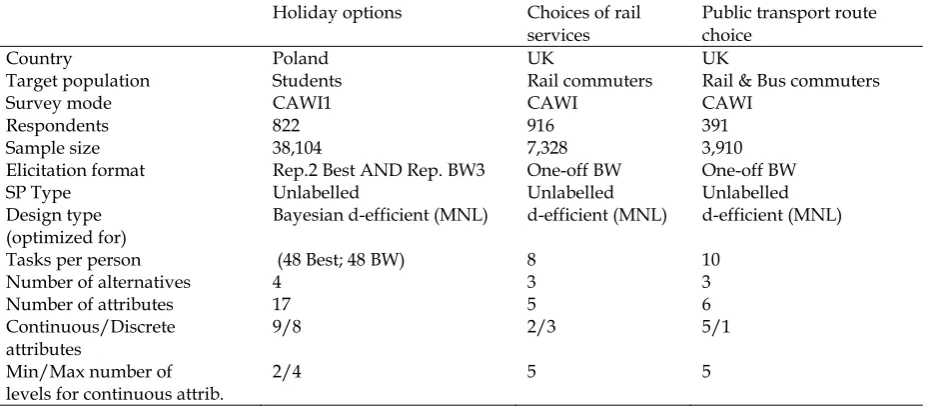
[image:7.595.68.538.211.415.2]In this paper, we use datasets from three studies varying in context, elicitation format, tasks per person, sample size, numbers of attributes and types of attributes. The studies are summarised in Table 2. We centre our data description around the holiday choice dataset as it provides the richest level of information and allows exploring our first research objective (differences in observed rank-orders between repeated best and repeated best-worst surveys). For further details on the second and third dataset, the interested reader is referred to Hess et al. (2012).
Table 2. Summary of datasets
Holiday options Choices of rail
services
Public transport route choice
Country Poland UK UK
Target population Students Rail commuters Rail & Bus commuters
Survey mode CAWI1 CAWI CAWI
Respondents 822 916 391
Sample size 38,104 7,328 3,910
Elicitation format Rep.2 Best AND Rep. BW3 One-off BW One-off BW
SP Type Unlabelled Unlabelled Unlabelled
Design type (optimized for)
Bayesian d-efficient (MNL) d-efficient (MNL) d-efficient (MNL)
Tasks per person (48 Best; 48 BW) 8 10
Number of alternatives 4 3 3
Number of attributes 17 5 6
Continuous/Discrete attributes
9/8 2/3 5/1
Min/Max number of levels for continuous attrib.
2/4 5 5
1CAWI – Computer Assisted Web Interview; 2Repeated; 3BestWorst
The holiday choice study was conducted on a sample of 822 students from the University of Warsaw. Over the course of one month, the students were requested to participate in nine independent sessions of the same stated choice experiment. In each session they were presented with sixteen choice tasks making a total of 144 observations per student.
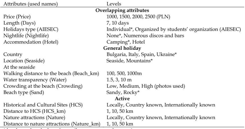
Each session focussed on a particular type of holiday, namely general holiday, holiday at the seaside or an active holiday. Each holiday type was described by five overlapping attributes: price, length, tour operator, nightlife and accommodation. In addition, a number of holiday type specific attributes were included. The full list of attributes and their corresponding levels is presented in Table 3. Three out of the nine sessions were dedicated to each holiday type, using the different elicitation formats. In each choice task, four options were presented for the specific holiday context.
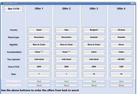
The elicitation format focused on the full preference ordering over the four alternatives, and respondents were asked to provide this in three different choice formats, namely (i) best-worst-best, (ii) best-best-best-worst-best, and (iii) free to determine (any combination of best and worst). Figure 1 provides an example of the free to determine case (first stage).
stage for every elicitation format, respondents could go one step back and change a response. Irrespective of the elicitation format, the full rank-order over the four alternatives was elicited and the different approaches can therefore result in the same rank-order. A third of the sample started with repeated BW, a third with repeated best questions and the final third started by selected the best and worst alternatives in their preferred order. In the analyses, we particularly focus on the repeated BW and repeated best datasets.
[image:8.595.72.525.211.524.2]All the choice tasks come from the same experimental design. The holiday choice dataset therefore allows conducting detailed tests comparing the stability of the parameters of interest across stages and between the alternative elicitation formats at the sample level.6
Figure 1. Example of choice scenario in the general holiday session
6 The respondents answered different choice tasks across the three elicitation formats. All respondents faced the
Table 3. Experimental design setup for the holiday dataset
Attributes (used names) Levels
Overlapping attributes
Price (Price) 1000, 1500, 2000, 2500 (PLN)
Length (Days) 7, 10 days
Holidays type (AIESEC) Individual*, Organized by students’ organization (AIESEC)
Nightlife (Nightlife) None*, Numerous discos and bars
Accommodation (Hotel) Camping*, Hotel
General holiday
Country Bulgaria, Italy, Spain, Ukraine*
Location (Seaside) Seaside, Mountains*
At the seaside
Walking distance to the beach (Beach_km) 100, 500, 1000m
Water transparency (Water) 1.5, 3, 10 m
Crowding at the beach (Crowding) Beach type (Sand)
Low, Medium, High (photos used) Sandy, Rocky*
Active
Historical and Cultural Sites (HCS) Locally, Country known, Internationally known
Distance to HCS (HCS_km) 1, 10, 50 km
Nature attractions (Nature) Locally, Country known, Internationally known
Distance to nature attractions (Nature_km) 1, 10, 50 km * levels used as the base for attributes not treated as continuous.
4. Empirical results
Section 4.1 contrasts the observed rank-orders obtained through the different elicitation formats used in the holiday dataset. Section 4.2 then proceeds by applying our various tests on the repeated best and repeated BW responses provided in the holiday dataset. The section follows the model specifications and statistical tests as described in Section 2. Section 4.3 provides a similar exercise for the two datasets using the one-off BW elicitation format.
4.1 Observed rank-orders in the holiday dataset
The application of the repeated best and repeated BW elicitation format in the holiday dataset provides a unique opportunity to investigate potential differences in response patterns as the same experimental design and the same respondents are used in both samples.
For each choice task in the experimental design we count the frequency at which a given alternative in that given task is ranked as either the first, second, third best or worst alternative; and how often a specific rank-order occurs. By comparing counts between the two samples, we find that in 93.8% of the cases (see Table 4), the first (best) alternative is the same. The discrepancy of 6.2% can be attributed to some randomness in choice behaviour. Very similar rates apply to the three remaining ranks. The exact same rank-order across the four alternatives in both formats is, as expected, lower, but still high at 86.4%.
Table 4. Comparison of preference orderings between repeated best and repeated BW First-
best
Second- best
Third- best
Fourth-best (Worst) Equality between repeated best and
repeated BW
93.8% 92.6% 92.5% 93.9%
Pearson’s 𝜒2 test
𝜒2 statistic 435.6 578.9 604.8 484.1
d.f.1 573 575 574 573
p-value 0.99 0.45 0.18 0.99
1 There are 4 possible orderings at each stage and 144 choice tasks hence the contingency table has a dimension of
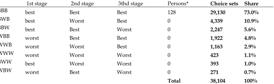
[image:9.595.78.531.632.724.2]These descriptive statistics illustrate that the same subjects, whilst presented with choice tasks from the same experimental same design but using two different elicitation formats, order alternatives in a very similar way. A non-parametric Pearson’s chi-square test presented in Table 4 confirms that preference ordering is independent of the elicitation format. The results are in sharp contrast with Rose (2014) who argues that the framing of the choice questions in terms of identifying the best or worst alternative is most likely to have an impact on choice behaviour. The observation that the elicitation format has no significant influence on the observed rank-orderings makes us wonder whether respondents have a preference for using the repeated best or repeated BW elicitation format. As a side step, we briefly focus on the unused sample in the holiday dataset where people could decide themselves whether to select a best or a worst alternative in each stage. It is striking from Table 5 that in 73% of all choice situations the repeated best response pattern was observed and in only 11% the repeated BW format. At the individual level, respondents tended to vary in their preferred approach across the 48 choice tasks in the experimental design. Surprisingly, only 128 (15%) respondents consistently used the same response pattern and they all consistently identified the best alternative. The detailed results on observed response patterns are reported in Table 5. It should be acknowledged that the observed response patterns do not necessarily imply a preference by people to respond in a repeated best fashion. Notably, Dyachenko et al. (2014) suggest that despite people first clicking on the best alternative, most likely they have already identified the worst alternative in the choice set.
Table 5. How choice tasks were answered in the free-ordering sample in the holiday dataset
1st stage 2nd stage 3thd stage Persons* Choice sets Share
BBB best Best Best 128 29,130 73.0%
BWB best Worst Best 0 4,339 10.9%
BBW best Best Worst 0 2,247 5.6%
WBB worst Best Best 0 1,922 4.8%
WWB worst Worst Best 0 1,163 2.9%
WWW worst Worst Worst 0 423 1.1%
BWW best Worst Worst 0 393 1.0%
WBW worst Best Worst 0 271 0.7%
Total 38,104 100%
*Number of respondents consistently using this response pattern across all 48 choice tasks
4.2 Empirical results for repeated best and repeated BW
Section 4.1 indicated that respondents may have a preference for using a repeated best elicitation format, but most importantly that the observed rank-orders do not differ significantly between the repeated best and repeated BW elicitation format. Based on the latter, one would expect that if the stability of utility parameters does not hold for the repeated best sample, it is also unlikely to hold for the repeated BW sample.
4.2.1 Contrasting the repeated best and repeated best-worst sample
To start the parametric analysis, we present the results for model specification II in Table 6.
Results for model specifications I, III and IV are available upon request from the authors. In all model specifications, robust standard errors account for the panel nature of the data (cf. Daly & Hess, 2011). The results are presented for MNL model specifications to facilitate explanation, but mixed logit models have also been estimated and confirmed the MNL results.
choice complexity. Decreasing scale parameters (i.e. higher variance) were therefore interpreted asevidence that later stages, i.e. decisions over lower ranked alternatives, are more complicated. Following similar logic, Scarpa et al. (2011) claimed that repeated BW is superior to repeated best since the first stages in this format were associated with high scale parameters (low variance) even though the choices are made over a larger set of alternatives and cover the lowest rank. Scarpa et al. (2011) stated that cognitive facilitation associated with the BW approach makes the elicitation format more appropriate.
[image:11.595.80.524.349.684.2]At first sight, the scale parameters reported in Table 6 are in accordance with Scarpa et al. (2011). For the repeated best format, we indeed observe in column 2 a decrease in scale after the first stage. Remember that for the first stage the scale parameter is normalised to unity. The worst (second) stage in the BW sample, on the contrary, is associated with the same scale parameter as the first (best) stage (see column 8). Interestingly, these observations reverse when the underlying exploded logit models treat the data ‘as if’ using the alternative elicitation format (see respectively columns 4 and 6). This recoding exercise is possible since the full rank-order was elicited. The results suggest that part of the advocated advantage of repeated BW over repeated best can be attributed to changes in the underlying econometrics, such as choice task composition and asymmetric error terms (e.g. de Palma et al. 2017), rather than to a framing effect (i.e. cognitive facilitation).
Table 6. Model estimates for model specification II before and after recoding
Sample used Repeated best Repeated BW
Exploded logit coded as Repeated best Repeated BW Repeated best Repeated BW
coeff t-stat coeff t-stat coeff t-stat coeff t-stat
Hotel 0.52 21.78 0.52 20.81 0.51 21.02 0.52 21.45
AIESEC 0.09 3.97 0.10 4.67 0.10 4.68 0.09 3.89
Beach_km -0.43 -22.56 -0.44 -21.69 -0.45 -22.15 -0.42 -22.13
Price -2.19 -42.77 -2.13 -43.90 -2.13 -43.73 -2.19 -42.99
Bulgaria 0.55 15.65 0.52 15.14 0.55 15.63 0.52 15.55
Italy 1.09 24.26 1.07 24.73 1.11 25.22 1.05 23.86
Spain 1.18 27.06 1.15 26.85 1.18 27.09 1.14 26.99
Crowding -0.25 -16.47 -0.26 -16.24 -0.25 -15.53 -0.26 -17.11
HCS 0.38 18.75 0.40 19.72 0.41 20.22 0.38 18.23
HCS_km -0.01 -19.05 -0.01 -21.56 -0.01 -20.41 -0.01 -20.22
Days 0.15 25.92 0.16 27.51 0.16 27.56 0.15 25.81
Nature 0.27 16.96 0.29 17.54 0.28 16.91 0.27 17.39
Nature_km 0.00 -7.81 0.00 -7.85 -0.01 -9.51 0.00 -5.94
Nightlife 0.40 18.06 0.40 17.98 0.41 18.48 0.39 17.42
Sand 0.66 19.93 0.66 19.95 0.66 19.79 0.67 20.11
Seaside 0.58 14.49 0.57 14.57 0.56 14.14 0.60 15.00
Water 0.03 8.60 0.03 9.99 0.03 10.34 0.03 8.18
acs2 -0.06 -4.75 -0.06 -5.24 -0.05 -4.60 -0.06 -5.30
asc3 0.02 1.67 -0.04 -3.29 -0.01 -1.36 -0.01 -0.55
asc4 -0.07 -5.64 -0.04 -4.05 -0.03 -2.99 -0.08 -6.67
scale2 0.83 15.52 1.00 0.07 0.84 14.68 1.02 1.79
scale3 0.87 8.72 0.57 29.14 0.83 10.07 0.56 25.96
LL -93,178.26 -94,087.86 -94,076.28 -93,234.64
N 822 822 822 822
Obs 38,104 38,104 38,104 38,104
cultural sites (Cult_km) the difference is significant at the 5% significance level (see column 2 in table 8). After accounting for differences in the exploded logit model none of the differences in WTP are significantly different between the two samples (see respectively columns 4 and 6 in Table 8).
Table 7. WTP estimates depending on the assumed exploded logit model
Sample used Repeated best Repeated BW
Exploded logit coded as Repeated best Repeated BW Repeated best Repeated BW
WTP t-stat WTP t-stat WTP t-stat WTP t-stat
Hotel 237.15 18.27 241.95 18.44 239.73 18.56 237.85 18.24
AIESEC 39.50 3.88 48.39 4.67 47.93 3.97 39.35 4.66
Beach_km -194.70 -19.29 -206.17 -20.01 -212.28 -19.81 -190.10 -19.50
Bulgaria 251.42 14.34 243.03 14.36 259.03 14.51 239.51 13.93
Italy 496.61 20.00 501.68 21.26 521.59 20.48 478.86 20.78
Spain 537.79 22.29 537.19 22.74 554.32 22.59 522.87 22.45
Crowd -113.02 -15.78 -121.19 -14.94 -116.03 -15.42 -118.42 -15.43
HCS 173.62 16.24 189.80 17.98 190.49 16.78 172.45 17.41
HCS_km -4.67 -19.47 -5.50 -19.25 -5.23 -18.19 -4.97 -20.35
Days 68.75 30.07 74.09 31.49 73.41 29.72 69.76 31.94
Nature 124.55 15.80 134.10 15.16 133.27 15.42 124.48 15.70
Nature_km -2.09 -5.80 -2.17 -9.20 -2.64 -7.60 -1.57 -7.61
Nightlife 182.38 15.75 187.26 16.46 191.16 16.26 177.24 16.08
Sand 299.16 17.37 310.96 17.51 307.61 17.42 304.72 17.48
Seaside 266.33 14.07 266.72 13.53 260.20 13.63 275.02 13.90
[image:12.595.72.523.414.634.2]Water 12.72 7.89 14.48 10.14 14.88 8.31 12.34 9.78
Table 8. Differences in WTP estimates depending on the assumed exploded logit model WTP difference between the Repeated best and Repeated BW sample using
Exploded logit coded as Original coding Repeated best coding Repeated BW coding
WTP t-stat WTP t-stat WTP t-stat
Hotel -4.79 -0.26 -2.58 -0.14 -4.10 -0.22
AIESEC -8.90 -0.62 -8.43 -0.59 -9.04 -0.62
Beach_km 11.47 0.79 17.59 1.22 16.07 1.11
Bulgaria 8.39 0.34 -7.61 -0.30 -3.52 -0.15
Italy -5.07 -0.15 -24.98 -0.72 -22.82 -0.67
Spain 0.60 0.02 -16.53 -0.49 -14.32 -0.43
Crowd 8.17 0.76 3.01 0.28 2.76 0.25
HCS -16.18 -1.08 -16.87 -1.14 -17.35 -1.14
HCS_km 0.83 2.23 0.56 1.50 0.53 1.41
Days -5.46 -1.67 -4.70 -1.43 -4.30 -1.31
Nature -9.55 -0.81 -8.71 -0.73 -9.62 -0.83
Nature_km 0.09 0.22 0.55 1.39 0.60 1.54
Nightlife -4.88 -0.30 -8.78 -0.54 -10.02 -0.62
Sand -11.80 -0.48 -8.45 -0.34 -6.25 -0.25
Seaside -0.39 -0.01 6.13 0.22 8.30 0.30
Water -1.76 -0.83 -2.16 -1.02 -2.14 -0.99
4.2.2 Detailed empirical tests of parameter stability
Test 1 lists the log-likelihoods for model specifications I-III. Model specification I contains twenty model parameters, since the two scale parameters used in model specification II are normalised to unity. For model specification III, sixty model parameters need to be estimated since for each stage, twenty unique utility parameters are estimated.
The LR-test shows that model specification II controlling for scale heterogeneity fits significantly better than model specification I. More important, in both the repeated best and repeated BW dataset, model specification III significantly outperforms model specifications I and II. This result suggests that only controlling for differences in scale parameters is insufficient and that wrongfully assuming parameter stability across stages may lead to incorrect inferences. Hence, the warnings of previous research on pooling responses from repeated best surveys are confirmed and extend to pooling responses across stages from the repeated BW format.
Tests 2.1 and 2.2 look more closely into the compatibility of individual stages. Model specifications I-III are again estimated on both the repeated best and repeated BW dataset, but now for the three possible pairs of stages. The LR test fails to accept the null-hypothesis of equivalent utility parameters across every pair of stages. For all possible combinations of stages, the model allowing for stage specific utility parameters gives the better fit for the data. The
Bayesian Information Criterion (BIC) used in Test 2.2 penalises more heavily for additional parameters included in the model, but even under this criterion there is only a single case in which responses from two alternative stages can be jointly analysed. Namely, stage 2 (‘worst’) and stage 3 (‘best’) responses from BW can be combined as long as scale differences are taken into account.
Test 2.3 covers model specification IV, where preference and scale parameters are assumed to be constant across two stages, but are allowed to vary with respect to a third stage. The BIC results highlight that model specification III provides the best BIC in the repeated best dataset. For the repeated BW dataset, the best fit is associated with model specification IV when combining stages 2&3 with the first stage being treated differently. The BIC for this specification is slightly better than that for model specification III. In either elicitation format, selecting the first (best) alternative is conceived different from selecting alternatives at a lower rank, irrespective of the way in which these questions are framed. Similarities in response patterns may still occur in later stages, but are unlikely.
Test 3.1 Overall, we find that the WTP values are stable across stages in terms of sign and statistical significance, but not in terms of their actual levels. For most of the attributes there are large and significant differences in WTP across stages.7 In the repeated best dataset, WTP values
for stage 1 and 3 are systematically higher than for stage 2 (‘2nd best’). The direction of differences
in WTP between stages 1 and 3 is, however, not apparent. For repeated BW, the WTP values for stage 1 are in most cases higher than for stage 2 (‘worst’) and stage 3 (‘2nd best’), but the direction
of differences between stages 2 and 3, i.e. when comparing the lower ranks is not evident. These results confirm the model fit results where selecting the best alternative (stage 1 in repeated best; stage 2 in repeated BW) is significantly different from selecting alternatives at a lower ranking in the preference ordering. This result is in line with the results from Carlsson et al. (2012). In all, this makes joint analysis for efficiency purposes a risky exercise in both the repeated best and repeated BW elicitation formats.
Test 3.2 The WTP estimates based on model specification II significantly differ from the WTP estimates based on the first stage for four attributes for both elicitation formats. In both cases the direction of these differences indicates that relying on the model specification II will result in lower WTP estimates compared to the model estimated on best responses only. These results are consistent with Test 3.1.
7 Summary statistics are reported, giving the number of significant positive (“+”) and negative (“-“) differences,
Table 9. Testing parameter stability in the repeated best and repeated BW samples Test 1 – LR test
LL for model specification: LR – test between model specifications
I (df=20)
II (df=22)
III (df=60)
I vs. II p-value I vs. III p-value II vs. III p-value
Rep. B -93,321.15 -93,178.26 -92,832.44 285.79 0.00 977.43 0.00 691.64 0.00
Rep. BW -94,897.15 -94,087.86 -93,763.80 1,618.57 0.00 2,266.70 0.00 648.12 0.00
Test 2.1 – LR-test
LL for model specification: LR –test between model specifications
Stages I (df=20) II (df=21) III (df=40) I vs. II p-val I vs. III p-val II vs. III p-val
Rep.
B 1 & 2 1 & 3 -72,142.4 -59,776.5 -72,006.2 -59,713.0 -71,786.2 -59,547.7 127.0 272.4 0.00 0.00 712.4 457.6 0.00 0.00 330.6 440 0.00 0.00
2 & 3 -54,448.8 -54,442.7 -54,331.0 12.2 0.00 235.6 0.00 223.4 0.00
Rep.
BW 1 & 2 1 & 3 -70,331.3 -63,371.1 -70,331.3 -62,667.7 -70,085.2 -62,565.7 1,406.8 0.0 0.98 0.00 492.2 1,610.8 0.00 0.00 204 492.2 0.00 0.00
2 & 3 -55,620.4 -54,969.5 -54,876.7 1,301.8 0.00 1,487.4 0.00 185.6 0.00
Test 2.2 – BIC
BIC for model specification: Difference in BIC between model
specifications
Stages1 I II III I vs. II I vs. III II vs. III
Rep.
B
1 & 2 144,495.73 144,233.99 143,994.27 -261.73 -501.46 -239.72
1 & 3 119,763.96 119,647.51 119,517.31 -116.40 -246.64 -130.20
2 & 3 109,108.59 109,106.91 109,083.95 -1.68 -24.64 -22.96
Rep.
BW
1 & 2 140,873.46 140,884.01 140,592.40 10.54 -281.05 -291.60
1 & 3 126,953.07 125,556.96 125,553.35 -1,396.11 -1,399.71 -3.60
2 & 3 111,451.78 110,160.53 110,175.23 -1,291.25 -1,276.54 14.70
Test 2.3 - BIC
Repeated Best Repeated BW
Model specification df LL BIC BIC - BIC model III df LL BIC
BIC - BIC model III
I 20 -93,321.15 18,6853.27 555.50 20 -94,897.15 19,0005.27 1,844.77
II 22 -93,178.26 18,6588.58 290.81 22 -94,087.87 18,8407.79 247.30
III 60 -92,832.44 18,6297.76 - 60 -93,763.80 18,8160.49 -
IV - 1_2+3 41 -93,052.51 18,6537.49 239.72 40 -94,009.81 18,8441.55 281.06
IV - 1_3+2 41 -92,997.75 18,6427.96 130.20 41 -93,865.81 18,8164.10 3.60
Test 3.1 – WTP differences between stages
Repeated Best sample2 Repeated BW sample3
Direction Cases Mean Min Max Cases Mean Min Max
|WTP1|-|WTP2|
"+" 8 0.44 0.16 0.87 6 0.35 0.24 0.61
"-" 0 - - - 2 -0.39 -0.44 -0.35
"n.s." 8 8
|WTP1|-|WTP3|
"+" 4 0.26 0.16 0.48 8 0.33 0.20 0.78
"-" 5 -0.64 -1.31 -0.27 1 -0.49 -0.49 -0.49
"n.s." 7 7
|WTP2|-|WTP3|
"+" 0 - - - 3 0.49 0.42 0.64
"-" 9 -0.57 -1.27 -0.21 2 -0.47 -0.31 -0.63
"n.s." 7 5
Test 3.2 – WTP difference between stage 1 and model specification II
|WTP stage 1|- |WTP model II| Cases Mean Min Max
Rep B
es
t
4 "+" 4 0.22 0.19 0.31
"-" 0
"n.s." 12
Rep B
W
5 "+" 3 0.20 0.15 0.31
"-" 1 -0.24 -0.24 -0.24
"n.s." 12
1 The numbers: 1, 2, 3 stand for stage numbers. 2,3,4,5, All differences are expressed in relative terms with the
absolute value of WTP from 1st best being the base
4.3 Tests results for one-off BW data sets
The results for the other two datasets are summarised in Table 10. As discussed in Section 2.3, three alternative econometric approaches were followed. Besides estimating the MaxDiff model, the exploded logit model was also applied treating the data as if coming from repeated best-worst (BW) or repeated best-worst-best (WB) questions.
Test 1 – Regardless of the selected econometric approach, the LR test results are consistent with the findings for the holiday dataset. Allowing for stage specific utility parameters results in a significantly better model fit for model specification III and thereby rejects the notion of stability of utility parameters.
Test 1 – extended - The BIC values tell the same story as the LR-test for the rail services dataset. In the route choice dataset, accounting for differences in scale between best and worst responses (i.e. using model specification II) is sufficient when using the MaxDiff model or assuming a worst-best response order. When a repeated Best-Worst assumption is adopted, model specification I even provides the best BIC-criterion. The increase in fit is thus not large enough to overcome the penalty for including the additional utility parameters in model specification III. In short, the notion of utility parameter stability holds here when adopting a more stringent evaluation criterion than the LR-test, but only in one out of two datasets.
Furthermore, for the WiFi and Ticket Type attributes sign reversals (and non-significant marginal WTP estimates) are observed between the best and the worst stage. In all, the rail services dataset highlights that differences in marginal WTP estimates are present across the stages.
For the route choice dataset, we observe that the WTP values are stable in terms of signs and statistical significance, but still not in terms of their actual levels. Despite the BIC criterion suggesting that a generic model accounting for scale heterogeneity is sufficient for this dataset, we do observe some significant differences in marginal WTP estimates across stages. The pattern is consistent across econometric approaches showing that the marginal WTP for a reduction in average delay is higher when looking only at the best responses, whereas the crowding and rate of delay attribute become significantly higher when looking only at the worst responses. Non-significant differences are found for the value of time and information attributes. These results suggest that respondents may tend to focus more on the attributes associated with a bad experience when selecting the worst alternative in this case. The experimental designs do not allow to test such behavioural hypotheses in more detail.
Test 3.2 - As expected based on the previous tests, significantly different marginal WTP estimates are obtained for the rail services dataset by pooling all stages and comparing these against the WTP estimates from the first best choices. The directional effect of this difference is, however, not clear. For the route choice dataset, the risks of incorrect inference by imposing constant utility parameters across the stages are slightly smaller. We only observe a single significant difference (on random delay in the BW model) in marginal WTP estimates between the generic models’ marginal WTP estimates and the first (best) marginal WTP estimates. The LR-test presented in test 1 contrasting model fit is therefore not conclusive and stage specific marginal WTP parameters need to be contrasted to see whether there is a risk in the joint analysis of the data. Overall, the test results indicate that the notion of stable utility parameters stability which would allow us to jointly analyse responses to repeated best and worst questions or one-off BW questions is unlikely to hold. In both formats, significant differences in utility parameters and marginal WTP estimates across stages are observed. Only for the route choice dataset we find some evidence for stable preferences across the ranks. Accordingly, only a small difference when comparing the marginal WTP estimates from the first (best) option to the WTP from model specification II. We therefore find it hard to support the claim that BW formats (either repeated or one-off) are superior over repeated best questions.
5. Conclusions
Stated choice surveys have a long tradition in producing guidance for policy makers. The aim of the present paper was to investigate the benefits and potential pitfalls of the best-worst (BW) elicitation format, which has gained increasing attention in the recent SC literature. We specifically focussed on testing the stability of the utility parameters and the associated marginal willingness to pay (WTP) estimates across the stages of the BW elicitation format.
Our analysis used three datasets relying respectively on the repeated best, repeated BW and the one-off BW elicitation format. In one of the datasets, the repeated best and repeated BW format were directly contrasted. The results highlight that the observed rank-orderings are highly comparable and not significantly different from each other. Both elicitation formats, however, suffer from significant differences in utility parameters and marginal WTP estimates across stages. Similar observations are made for the one-off BW response format where respondents identify the best and the worst alternative in the same screen. For all elicitation formats, we observe that the WTP estimates from pooled models significantly differ from the WTP estimates based only on the first (best) answers. Our analyses thus make clear that, irrespective of the selected elicitation format, solely accounting for scale differences across the stages may not be sufficient. Researchers should be aware of the risks they are exposing themselves to when (wrongfully) assuming stability of utility parameters across stages.
According to some authors, studies based on BW tasks are believed to be superior to using a sequence of repeated best questions as they are thought to take advantage of a person’s propensity to respond more consistently to extreme options by moving the focus away from middle ranked alternatives. The BW approach thereby potentially circumvents the stability issues observed in the repeated best approach (see for example Flynn et al. 2007, and Marley 2010). These claims are often repeated in the literature, however, according to our knowledge, have not been carefully tested, with the exception of Scarpa et al. (2011). The latter paper showed that first stages using worst elicitation format were associated with higher scale parameters (lower variance). Based on this finding, Scarpa et al. (2011) state that cognitive facilitation associated with the BW approach makes this elicitation format more appropriate than standard ranking. In our paper, we find exactly the same pattern as in Scarpa et al. (2011) and Collins and Rose (2013). In addition, we show that the utility parameters and scale parameters from repeated best and repeated BW elicitation formats are highly comparable as long as the data coming from these two elicitation formats are re-coded into the same response format.
Table 10. One-off BW elicitation, results tests 1 – 3 Test 1 – LR test
LL for model specification: LR-test between model specifications
Ra
il
Ser
vices
Model I II III I vs. II p-value I vs. III p-value II vs. III p-value
BW -10,175.23 -10,138.98 -10,033.65 72.50 0.00 283.16 0.00 210.66 0.00
WB -10,159.54 -10,139.54 -10,021.59 40.00 0.00 275.90 0.00 235.90 0.00
Maxdiff -10,172.51 -10,170.51 -10,063.17 4.00 0.05 218.68 0.00 214.68 0.00
Rou
te
ch
oi
ce
BW -5,973.97 -5,972.28 -5,960.50 3.38 0.07 26.94 0.00 23.56 0.00
WB -5,962.56 -5,937.62 -5,925.01 49.88 0.00 75.1 0.00 25.22 0.00
Maxdiff -5,979.81 -5,970.18 -5,957.25 19.26 0.00 45.12 0.00 25.86 0.00
Test 2 – extended - BIC
BIC for model specification: Difference in BIC between model specifications
Model I II III I vs. II I vs. III II vs. III
Ra
il
Ser
vices
BW -20,394.96 -20,331.36 -20,156.29 -63.60 -238.66 -175.06
WB -20,363.58 -20,332.48 -20,132.17 -31.10 -231.40 -200.30
Maxdiff -20,389.52 -20,394.42 -20,215.33 4.90 -174.18 -179.08
Rou
te
ch
oi
ce
BW -11,997.57 -12,002.46 -12,020.26 4.89 22.69 17.80
WB -11,974.75 -11,933.14 -11,949.28 -41.61 -25.47 16.14
Maxdiff -12,009.25 -11,998.26 -12,013.76 -10.99 4.51 15.50
Test 3.1– WTP differences between stages
Rail Services Route choice
Cases Mean Cases Mean
BW |WTP_Best| - |WTP_Worst|2
"+" 13 0.93 1 1.86
"-" 1 -0.73 2 -0.28
"n.s." 0 - 2 -
WB |WTP_Worst| - |WTP_Best|
"+" 14 0.36 1 1.28
"-" 1 -0.76 2 -0.37
"n.s." 0 - 2 -
MaxDiff |WTP_Best| – |WTP_Worst|
"+" 13 1.18 1 3.81
"-" 1 -0.83 2 -0.43
"n.s." 0 - 2 -
Test 3.2 - WTP diff. stage 1 and model specification II
Rail Services Route choice
Cases Mean Cases Mean
BW |WTP_model_II|–|WTP_Best|
"+" 2 0.32 1 0.32
"-" 2 -0.75 0 -
"n.s." 0 - 4 -
WB |WTP_model_II|–|WTP_Best|
"+" 2 0.95 0 -
"-" 2 -0.66 0 -
"n.s." 0 - 5 -
MaxDiff |WTP_model_II|–|WTP_Best|
"+" 2 0.84 0 -
"-" 2 -0.74 0 -
"n.s." 0 - 5 -
1 For BW and WB models scale associated with the first stages was normalized to 1. For the MaxDiff model scale
associated with ‘best’ was normalized to 1.
2 All differences expressed in relative terms with WTP from the second stage being the base.
3 WTP values for two attributes change sign (ticket type and WiFi), being positive for ‘best’ and negative for
‘worst’. Relative results not reported.
4 WTP for one attribute (ticket type) changes sign from positive with ’best’ to negative with ‘worst’. WiFi is not
Acknowledgements
The authors are grateful for the comments of anonymous reviewers on earlier versions of this paper. Data collection and work conducted by the first and third author were supported by the Polish National Science Centre grant DEC-2012/07/E/HS4/04037. The second and third author would like to acknowledge the financial support by the European Research Council through the consolidator grant 615596-561 DECISIONS.
References
Anderson, S.P. and de Palma, A. (1999). Reverse discrete choice models. Regional Science and Urban Economics, 29(6), 745-764.
Ben-Akiva, M., Morikawa, T. and Shiroishi, F. (1991). Analysis of the reliability of preference ranking data. Journal of Business Research, 23(3), 253-268.
Bradley, M. and Daly, A. (1994) Use of the logit scaling approach to test for rank-order and fatigue effects in stated preference data. Transportation, 21(2), 167-184.
Chapman R, Staelin R (1982). Exploiting rank ordered choice set data within the stochastic utility model. Journal of marketing research, 14, 288-301.
Carlsson F, Mørkbak MR, Olsen SB (2012) The first time is the hardest: a test of ordering effects in choice experiments. Journal of Choice Modelling, 5(2), 2012: 19-37.
Collins, A.C. and Rose, J.M. (2013) Estimation of stochastic scale with best-worst data, Paper presented at the 92rd Annual Meeting of the Transportation Research Board, Washington D.C.
Daly, A.J. & Hess, S. (2011), Simple Approaches for Random Utility Modelling with Panel Data, 90th Annual Meeting of the Transportation Research Board, Washington, D.C.
Dumont, J., Giergiczny, M. & Hess, S. (2015), Individual‐level models vs. sample‐level models: contrasts and mutual benefits, Transportmetrica A: Transport Science, 11(6), 465‐483
de Palma, A., Kilani, K., & Laffond, G. (2017). Relations between best, worst, and best-worse choices for random utility models. Journal of Mathematical Psychology, 76, 51-58.Dumont, J., Hess, S. and Giergiczny, M. (2015) Individual level models vs. sample level models: contrasts and mutual benefits.
Transportmetrica A, 11(6), 465-483.
Dyachenko, T., Reczek, R. W., & Allenby, G. M. (2014). Models of sequential evaluation in best-worst choice tasks. Marketing Science 33(6), 828-848.
Dumont, J., Giergiczny, M. & Hess, S. (2015), Individual‐level models vs. sample‐level models: contrasts and mutual benefits, Transportmetrica A: Transport Science, 11(6), 465‐483
Flynn TN, Marley AAJ (2014). Best worst scaling: Theory and methods. In: Hess S, Daly A (eds)
Handbook of choice modelling. Edward Elgar Publishing, UK.
Flynn, T.N., Louviere, J.J., Peters, T.J., Coast, J., (2007). Best-worst scaling: What it can do for health care research and how to do it. Journal of Health Economics, 26, 171-189.
Fok D, Paap R, Van Dijk B. (2012) A rank ordered logit model with unobserved heterogeneity in ranking capabilities. Journal of Applied Econometrics, 27, 831–46.
Foster, V., and S. Mourato. (2002). Testing for Consistency in Contingent Ranking Experiments. Journal of Environmental Economics and Management, 44(2), 309–28.
Hausman, J., Ruud, P., 1987. Specifying and Testing Econometric Models for Rank-Ordered Data.
Journal of Econometrics, 34, 83-103.
Hess, S., A. Stathopoulos, D. Campbell, V. O’Neill, and S. Caussade., (2012). It’s Not That I Don’t Care, I Just Don’t Care Very Much: Confounding Between Attribute Non-attendance and Taste Heterogeneity. Transportation 40 (3): 583–607.
Lancsar, E., Louviere, J. J. (2009). Estimating individual level discrete choice models and welfare measures using best worst choice experiments, CenSoC Working Paper, No. 08-003, University of Technology, Sydney.
Lancsar, E., Louviere, J., Donaldson, C., Currie, G., and Burgess, L. (2013) “Best worst discrete choice experiment in health: Methods and an application” Social Science and Medicine, 76, 74-82.
Louviere, J. J., Street, D., Burgess, L., Wasi, N., Islam, T., & Marley, A. A. J. (2008). Modeling the choices of individual decision-makers by combining efficient choice experiment designs with extra preference information. Journal of Choice Modelling, 1, 126-163.
Marley, A. A. J. (2010) The best-worst method for the study of preferences: Theory and Application.
In Cognition and Neuropsychology: International Perspectives on Psychological Science (Volume 1), edited by Peter A. Frensch & Ralf Schwarzer. Hove: Psychology Press, 147-157.
Marley, A. A. J., and Louviere, J. J. (2005). Some probabilistic models of best, worst, and best-worst choices. Journal of Mathematical Psychology, 49, 464-480.
Marley, A. and Pihlens, D. (2012). Models of best-worst choice and ranking among multiattribute options (profiles). Journal of Mathematical Psychology, 56(1), 24-34.
Marley, A. A. J., & Islam, T. (2012). Conceptual relations between expanded rank data and models of the unexpanded rank data. Journal of Choice Modelling, 5, 38-80.
Palma, M.A. (2016). Improving the prediction of ranking data. Empirical Economics, 1-30.
Rose, J.M. (2014), Interpreting discrete choice models based on Best-Worst data: A matter of framing,
Paper presented at the 93rd Annual Meeting of the Transportation Research Board, Washington D.C.
Scarpa, R., Notaro, S., Louviere, J., Raffaelli, R., (2011). Exploring scale effects of best/worst rank ordered choice data to estimate benefits of tourism in Alpine grazing commons. American Journal of Agricultural Economics 93, 813–828.