Characterizing ice particles using two-dimensional reflections of a lidar beam

Characterizing ice particles using

two-dimensional reflections of a lidar beam

M. G

,

Z. U

,

* G. R

,

E. H

,

R. R. N

III,

L. T

,

R. A. S

,

P. H. K

1_{Summit Station (Greenland), Polar Field Services, 8100 Shaffer Parkway, Littleton, Colorado 80127, USA}

2_{School of Physics Astronomy and Mathematics, University of Hertfordshire, Hatfield AL10 9AB, UK}

3_{National Centre for Atmospheric Science and the School of Earth and Environment, University of Leeds, Leeds LS2 9JT, UK}

4_{Department of Aerospace Engineering Sciences, University of Colorado, Boulder, Colorado 80309, USA}

*Corresponding author: [email protected]

Received 16 February 2017; revised 30 April 2017; accepted 30 April 2017; posted 1 May 2017 (Doc. ID 286882); published 19 June 2017

We report a phenomenon manifesting itself as brief flashes of light on the snow’s surface near a lidar beam. The flashes are imaged and interpreted as specular reflection patterns from individual ice particles. Such patterns have a two-dimensional structure and are similar to those previously observed in forward scattering. Patterns are easiest to capture from particles with well-defined horizontal facets, such as near-horizontally aligned plates. The pat-terns and their position can be used to determine properties such as ice particle shape, size, roughness, alignment, and altitude. Data obtained at Summit in Greenland show the presence of regular hexagonal and scalene plates, columns, and rounded plates of various sizes, among others.

Published by The Optical Society under the terms of theCreative Commons Attribution 4.0 License. Further distribution of this work must maintain attribution to the author(s) and the published article’s title, journal citation, and DOI.

OCIS codes:(010.1290) Atmospheric optics; (280.0280) Remote sensing and sensors; (290.0290) Scattering; (010.2940) Ice crystal phenomena; (030.6140) Speckle.

https://doi.org/10.1364/AO.56.00G188

1. INTRODUCTION

Atmospheric ice crystals are recognized to play a very important role in the interaction of electromagnetic radiation with the Earth’s atmosphere. This interaction depends crucially on ice crystal size and shape, the latter posing special difficulties because of its tremendous variety, which is hard to both measure and represent in models. Therefore, detailed characterizations of ice and modeling of the scattering are important components of atmospheric science [1,2]. Ice crystals are also the source of a variety of beautiful atmospheric optical phenomena, collectively known as ice halos. These halos originate principally from refrac-tion of light through ice crystals, the facets of which can have well-defined angles with respect to each other, such as 60° (pro-ducing the 22° halo) or 90° (for the 46° halo). However, less frequent halos are associated with reflections, such as the sun pillar produced by horizontally aligned plates [3]. Apart from their aesthetic value, halos can provide information about atmos-pheric ice, as different types are associated with different shapes, sizes, and orientations [4,5]. Conversely, their relative rarity has provided indications that atmospheric ice particles frequently do not possess the idealized hexagonal prism shape [2,3,6].

Halo-like features in scattering from individual crystals, for example, as manifested in two-dimensional (2-D) light scattering patterns, can be the basis for ice particle characterization. For

example, the strength of the 22° halo peak in scattering is an indication of how regular ice crystals are [7,8]. A more complete attribution of the shape is possible by comparing 2-D scattering patterns from individual ice crystals to the theory [9].

Polar regions are obviously of special importance because of their lower temperatures, favoring the presence of ice particles with their variety of shapes and sizes. They also pose excep-tional logistic and technical difficulties. Passive remote sensing from space becomes more problematic over bright snow or ice surfaces. Moreover, atmospheric ice can be present down to the

ground level, either generated in situ or as blown snow.

Satellite-based measurements become more challenging due to both these factors, and ground-based active remote-sensing measurements cannot simultaneously cover the lowest layer at the same time as upper layers. Notwithstanding the difficulties, much effort has been devoted to establishing ground-based observing stations in both the Arctic and the Antarctic—for a review of polar tropospheric lidar studies, see [10].

Atmospheric ice present at low altitudes can have consider-able impact on the energy balance. Blowing snow events with high optical depth can increase downward longwave radiation

by up to 30 W∕m2 [11]. During the nighttime, upwelling

longwave radiation (ULR) is usually larger when blowing snow is present, because the blowing snow is warmer than the surface

G188 Vol. 56, No. 19 / July 1 2017 /Applied Optics Research Article

due to the existence of surface-based inversion. The average difference in ULR with and without blowing snow over the

East Antarctic Ice Sheet was about 5 W∕m2 for the winter

months of 2009 [12]. Radiometry measurements in the Canadian high Arctic showed that a geometrically thin, low ice cloud resulted in a 6% increase in downwelling longwave irradiance [13].

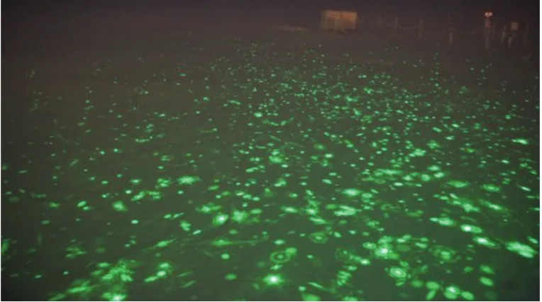
We report here observations of a phenomenon manifesting itself as brief flashes of light on the snow’s surface in the vicinity of a strong visible lidar beam. When photographed, the flashes reveal a 2-D structure reminiscent of scattering patterns ob-served in forward scattering and used for characterizing cloud and aerosol particles. A typical example of multiple reflections collected over a timespan of 39 s is shown in Fig.1.

Apparently, similar lidar reflections originating from a cloud layer 100 m above the Arctic snow surface were evocatively de-scribed as a multitude of“fireflies”by Hoff in 1988, who also con-jectured that the spots were specular reflections from crystal facets [14]. The phenomenon was later photographed by Marichevet al. [15], who also provided a simple geometric interpretation but did not suggest quantitative characterization of the ice crystals.

We quantify our observations by deriving the properties of the ice crystals, like the altitude and alignment angle, from the position of the 2-D patterns on the snow, compare the patterns to the scattering theory to retrieve the size and shape of the ice crystals and obtain the size of some of the crystals using a technique based on laser speckle [16].

2. METHODS

The measurements were made at Summit, Greenland (72°35046.40N,38°25019.10W, 3212 m above sea level) during the Arctic night of 2016/17. The illumination of the ice crystals was provided by the Cloud, Aerosol Polarization and Backscatter Lidar (CAPABL, 532 nm wavelength, pulse energy

60 mJ, pulse rate 15 Hz) [17,18]. The beam zenith angle was 32°—this large tilt eliminates from the receiver specular reflec-tions from near-horizontal ice plates and permits CAPABL to assess whether the observed ice crystals are horizontally or ran-domly oriented by measuring diattenuation [17,19]. At the time of the observations shown here, the lidar beam window was 4 m above the snow surface.

CAPABL and the other ancillary instruments providing ob-servations used in this study are located at Summit as part of the NSF-funded Integrated Characterization of Energy, Clouds, Atmospheric State, and Precipitation at Summit (ICECAPS) project [20]. The goal of ICECAPS is to make an assessment of how clouds and atmospheric processes impact the surface energy and hydrological budgets of the central Greenland Ice Sheet. In addition to CAPABL, the observations from twice daily radiosondes (Vaisala RS-41) and millimeter-wave cloud radar (MMCR) [21] have helped provide context to the occur-rence of the observed flashes. The MMCR is a zenith-pointing Doppler single-polarizationK_a-band (35 GHz) radar with a 2 s time resolution and 45 m vertical resolution. Precipitating ice particles were also collected on microscope slides and photo-graphed using the IcePic microscope, which is kept at ambient surface temperatures [20]. The temperature and humidity at 2 m above ground were measured using a Vaisala HMP155 probe with a capacitative sensor; the uncertainty of the relative humidity was 2%.

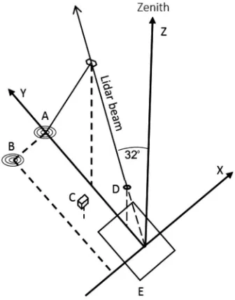
The 2-D patterns were photographed with a 6D Canon DSLR camera with a 24 mm focal length lens, f/2.8 aperture, and a sensitivity of 25600 ISO. Figure2shows the layout of the observations and the coordinate system used to determine the 2-D pattern locations. The camera was at a height of 1.5 m

above the snow surface, at location X −3 m, Y 4.5 m

in the coordinates in Fig. 2. Typical exposure times were

between 0.6 and 1.3 s. Pattern dimensions and distances were determined by placing a tape measure at known locations in

test images of the same field of view and interpolating pattern scales and locations using this data, taking into account the camera position. Individual pattern images were corrected for the influence of the viewing angle by expanding their ver-tical dimension anamorphically, taking into account the pattern distance and camera height. However, no account was taken of terrain curvature (though it is minimal), image skew, or camera lens distortion, so it is likely that the scaling and shape of some of the images are imprecise.

The altitude of ice crystals can be estimated from the 2-D pattern locations, assuming that the facets producing the specu-lar reflections are aligned horizontally as Z Y∕2 tanβ,

where Y is the distance of the pattern from the line on the

ground passing through the base of the lidar beam and normal to it (theX axis), andβ32° is the zenith angle of the beam. Due to the “shadow”of the roof surrounding the CAPABL’s

window ice particles producing patterns at Y <5.9 m (or

altitudes between the beam aperture and 4.7 m), we could not cast reflections onto the snow surface had they been hori-zontal. Nearly half of the patterns were found in this shadow region, although this high proportion is biased by the prefer-ence to select patterns near the camera, which was at coordinate Y 4.5 m, 1.4 m back from the edge of the shadow at Y 5.9 m—see Fig.4. Therefore, the patterns were assumed to originate from tilted facets, for simplicity, at an angle of 16°, so that their reflections propagated vertically down. For tilted facets, the formula for the altitude becomes: Z Y∕tan βtanβ−2δ, whereδis the tilt angle about theX-axis with respect to the horizontal orientation. Hence, for reflections propagating vertically in the shadow the altitude was Z Y∕tan β. The sideways tilt of the ice crystals, i.e., the

angle between the normal of the facet and the vertical plane containing the lidar beam, can be obtained as ρ≈arctanX∕2Z, whereXis the distance of the pattern from

the beam projection onto the ground (theY-axis).

For particles that are sufficiently rough or complex to pro-duce 2-D scattering patterns with significant speckle, it is possible to obtain the size from the size of the speckle spots. The particle sizeD, understood as the diameter of a circle with the same area as the cross section of the particle as seen in the incident direction, has been shown using measurements on a variety of particles to be inversely proportional to the median area of speckle spots in forward scattering. For the lidar wave-length, this relationship can be stated by the formula D45.3∕Ω, whereΩis the area expressed in degrees squared [16]. Since it is not clear at this stage if a different relationship may hold for scattering into the backward hemisphere, the original expression is used.

Theoretical 2-D patterns were computed using the ADDA discrete dipole approximation code [22] for particles with a

maximum dimension up to 60 μm, including rounded and

rough ones. An approximate method based on beam tracing with diffraction was used for larger particles with flat facets [23,24]. The beam tracing method was verified against

ADDA for hexagonal plates 60μm in diameter. The ADDA

computations were carried out on the University of Hertfordshire and UK ARCHER high-performance computing facilities, using between 16 and 208 processors. A wavelength

of 532 nm and a refractive index of1.31170iwere assumed

(the imaginary part is negligibly small at this wavelength).

3. OBSERVATIONS

The reflected 2-D patterns were photographed on the 6th December 2016 from 1851 to 2110 UTC. We obtained 2500 camera images, each typically containing between 0

and 3 individual patterns in the proximity to the camera—

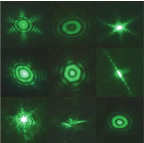
the entire data set can be seen as a time-lapse video in Visualization 1. We extracted 106 patterns from these images as a sample representative of different pattern types, and out of these, 40 were selected for further analysis on the basis of the presence of characteristic features recognizable from previous forward scattering data [8,9,16] as corresponding to faceted, rounded, or rough particles—a selection is shown in Fig. 3. The positions of these patterns are shown in Fig.4.

The sky was overcast, temperature was −180.4°C near

ground level, and the southwesterly wind speed was 9 m/s. Light-to-moderate precipitation was noted, and visibility was ∼1 km. The humidity w.r.t. ice recorded at a 2 m height during that period was slightly below the saturation level, with a mean of 96%, a minimum of 94%, and a maximum of 97%.

A later meteorological radiosonde sounding at 2315 UTC showed the presence of a sharp inversion at∼200 m. The tem-perature and relative humidity at 12 m were−18.6°Cand 86%

with respect to water, or ≈102% w.r.t. ice, i.e., close to

saturation—Fig.5. At that time, the ground station tempera-ture was−18.7°C, and the humidity w.r.t. ice was 98% at 2 m. The sounding indicated that the humidity was higher at the inversion and in some higher layers than near the ground, substantially exceeding the ice saturation.

Fig. 2. Cartesian coordinate system for locating the 2-D patterns. The snow surface is on theX Y (Z 0) plane, and the lidar beam is on theY Z (X 0) plane. Point A is the location of a specular re-flection for a horizontal ice plate, B for a plate tilted about theY-axis, C the location of the camera (X −3,Y 4.5,Z1.5 m), D the lidar aperture (X 0,Y 2.5,Z4 m), and E the footprint of the lidar hut.

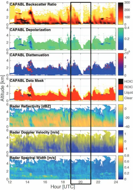
In Fig. 6, observations from CAPABL and the MMCR show conditions before, during, and after the photographs were taken. The observations show the presence of an ice cloud with a diffuse top at∼5 kmthat precipitated snow lightly through-out the entire period. CAPABL’s depolarization and strong di-attenuation (red coloring in Fig.6) observations also suggest that the cloud contained some horizontally orientated ice crystals (HOICs). Because CAPABL makes observations at a

large tilt angle, far from the zenith, the specular reflections nor-mally associated with HOICs are not found in its data. All of

CAPABL’s observations are combined into a data mask to

classify the bulk properties of the observations [18]. In Fig. 6, ice is shown in red, and horizontally oriented ice is shown in black. As mentioned in the introduction, the lowest section of CAPABL’s observations are missing because of the system’s overlap function, so signals returned by the ice crystals in this range are not seen by CAPABL’s detectors.

Particle altitudes, calculated for the 40 selected patterns as described in the Methods section, extended up to 22.5 m, with a mean value of 7.2 m. The retrieved orientation angles of the facets responsible for the reflections had a standard deviation of 6°, with a non-zero mean of −4°, attributable to bias due to pattern proximity to the camera, which was lo-cated atX −3 m, thus favoring negative alignment angles. Reconstructing a less biased distribution with a mean of 0° by taking negative tilts only and mirroring them in the positive half gave only a slightly larger standard deviation of 8°.

4. COMPARISONS TO THE SCATTERING THEORY

The observed patterns showed similarity to the diffraction pat-terns on the apertures of various shapes: rectangular, circular, and hexagonal, hinting at the shape of the ice crystal facets. There was also similarity to scattering patterns for particles with hexagonal facets, in forward scattering [9] and in backscattering in the specular reflection direction, with the phase angle cor-responding to twice the angle of incidence on a facet [23].

Fig. 3. Representative selection of individual patterns observed at Summit Station on 6 December 2016. The patterns were stretched anamorphically to correct for the viewing angle. The mean width of the visually discernible parts of the patterns was 1 m.

Fig. 4. Positions of 2-D patterns recorded on 6 December 2016 and analyzed to recover ice particle properties. The camera, lidar aper-ture, and roof shadow for the horizontal crystals (dashed line, see text) are also shown. The coordinates are as in Fig.2.

Light-scattering computations were carried out to visualize 2-D scattering in the vicinity of specular reflections from ice crystal facets and permit matching to the observations. Emphasis was on hexagonal plates for various sizes, aspect ratios, and degrees of rounding and roughness, but some computations for scalene plates and hexagonal columns were done, too. The example shown in Fig. 7is for a hexagonal plate with flat facets.

The initial assumption was that the observed patterns origi-nated from horizontally oriented crystals, supported by their observation earlier in the day by CAPABL’s polarization mea-surements. However, the geometric position of the patterns with respect to the lidar indicated that a significant proportion may have been tilted. The direct evidence was two-fold: the patterns fell away from the line directly below the lidar beam, and some of the patterns were within or close to the area that would have been in the shadow of the lidar hut had the crystals

been horizontal. Moreover, a comparison with theoretical pat-terns revealed that some observed patpat-terns could not be satis-factorily fitted, assuming the angle of incidence was equal to the lidar beam zenith angle (32°), corresponding to the horizontal

orientation. The difference can be seen by comparing Fig. 8

with Fig.9, where the incident angles are 32° and 20°, respec-tively, and the former pattern is clearly more elongated.

Fig. 6. CAPABL lidar and MMCR radar data from 1200 to 2400 UTC on 6 December 2016 at Summit; the camera imaging period is highlighted. The top three panels show the backscatter ratio (i.e., the ratio of total scattering to molecular scattering), depolarization, and diattenuation observed by CAPABL [17]. The middle panel is the cloud mask derived from CAPABL [18]. The bottom three panels show the reflectivity, Doppler fallspeed (where a positive value is downward), and the spectrum width (representative of turbulence or differential fall velocity). Since radar and lidar are complementary sensors that experience differing amounts of attenuation due to scatter by the cloud, CAPABL rarely observes the cloud top (∼5 km), while the radar is able to penetrate the entire layer.

Fig. 7. Left: pattern photographed at Summit, image width 5°, stretched anamorphically to compensate for the viewing angle. The pattern angular scale is approximate, based on particle altitude esti-mate. The observed image was stretched in the vertical direction to correct for the viewing angle. The particle diameter estimated from fringe separation was 150μm. Right: theoretical 2-D scattering pattern from a 50μm diameter, 1μm thick, hexagonal plate tilted at 32° w.r.t. the incident direction. The pattern is centered on the direction of the specular reflection from the basal facet and is 10° wide.

Fig. 8. Left: as in Fig.7, but the size is 130μm. Right: theoretical pattern from a 50μm diameter, 4μm thick, slightly rounded hexago-nal plate tilted at 32° w.r.t. the incident direction, image width 10°.

Fig. 9. Left: as in Fig.7, but the size is 120μm. Right: theoretical pattern for a strongly rounded hexagonal plate 50μm diameter, 1μm mean thickness, incident angle 20°, image width 20°.

Consequently, some particle altitudes, angular scales, sideways tilts, and scattering patterns were calculated for tilted particles, with angles of incidence<32°.

Some of the observed 2-D patterns indicated the presence of facets departing in shape from hexagonal symmetry, and a con-tinuum was seen through to patterns typical of diffraction on circular apertures—see Fig.3. Therefore, comparisons for mod-eled hexagonal plate-like particles with increasing rounding were carried out and are shown in Figs.7–10, with the corre-sponding particle shapes in Fig. 11.

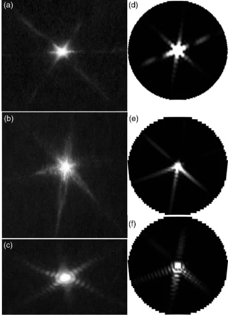
Since good matches could not always be obtained assuming regular hexagons, further calculations were done for scalene

plates, where alternate sides were shorter—the comparisons are shown in Fig.12, together with a counterexample of a regu-lar hexagonal plate [Fig.12(f )]. It is seen that indeed, a better fit can be obtained for the scalene shape.

Figure 13 shows a comparison with a hexagonal column

model. Figure 14 shows a comparison for a hexagonal plate

Fig. 10. Left: as in Fig.7, but the size is 175μm. Right: theoretical pattern for a 40 μm diameter, nearly spheroidal plate with 0.5μm mean thickness, incident angle 20°, image width 20°.

Fig. 11. (a)–(d): side-on and perspective views of the particle shape models used for computing the patterns shown in Figs. 7–10, respectively.

Fig. 12. Left: patterns from Summit, width 5° (a)–(c); pattern (c) corresponds to plate diameter of≈210μm. Right: patterns com-puted from beam tracing for scalene plates with 3.6 and 36μm edges, image width 16° (d), 9 and 91μm edges, image width 10° (e), and a 100 μm diameter regular hexagonal plate, image width 10° (f ), all 10μm thick.

with rough surfaces, where the standard deviation of the surface vertices was 0.075μm.

A broad range of particle sizes was apparent. Comparisons of patterns with a well-defined“diffraction”structure according to the theory, assuming an inverse linear relationship between the fringe spacing and particle (strictly speaking facet) size, were

consistent with diameters from 125 to 530μm, with a mean

of 190μm for plate-like particles, and 120 to 560μm lengths with a mean of 380μm for column-like particles. Patterns with complex speckle indicated larger sizes: 0.7 to 4.0 mm, with a mean of 2.5 mm.

5. DISCUSSION

We have presented observations of 2-D light scattering patterns on an Arctic snow surface due to interaction between a lidar beam and suspended ice particles. Close resemblance to theo-retical light scattering patterns confirms that the observed pat-terns are dominated by specular reflections from ice prism facets, modified by scattering effects. The data obtained at Summit are consistent with the presence of hexagonal ice plates and columns, among others. The positions of the 2-D patterns on the snow with respect to the lidar beam allows us to retrieve a measure of the“flutter”angle distribution of the ice crystals and, if the distribution is not too broad, also the altitude. The semi-quantitative comparison of the patterns to the scattering theory allowed us to retrieve the size and shape of the ice crystals and, for rough or complex crystals, the size, using a technique based on laser speckle.

About half of the plates showed evidence of rounding, in some cases so strong that hexagonal symmetry was no longer apparent, as the patterns resembled the familiar diffraction pat-terns on circular apertures. These shapes suggest that the crystals had undergone sublimation [25], even though the mea-sured relative humidity indicated saturation with respect to ice. Some 2-D patterns indicated the presence of scalene plates with unequal sides, as opposed to regular hexagonal plates—see Fig.12. This was confirmed by the scalenes seen in some IcePic images. This finding is important, because in addition to having different radiative properties, scalene crystals may be the indicators of the presence of stacking-disordered ice [26].

A significant proportion of the 2-D patterns, ≈10%,

showed pronounced speckle—see the examples in Figs. 3

and 14. For such patterns, the particle size can be estimated using a technique based on laser speckle [16]. This indicated relatively large sizes: 0.7 to 4.0 mm, with a mean of 2.5 mm. They presumably corresponded to precipitating snow, also seen in this size range on the IcePic microscope slides collected at the time of the observations. The amount of speckle present in 2-D patterns allows us to evaluate the degree of ice particle rough-ness or complexity, which is highly important from the viewpoint of the radiative properties of ice, as rough ice tends to have a lower scattering asymmetry parameter than smooth ice [8].

Thus, two distinct, apparently non-overlapping subpopula-tions of ice crystals were identified: fast precipitating snow par-ticles producing pronounced speckle, with sizes from 0.7 to 4.0 mm, and pristine ice particles consisting of smaller plates

between 125 and 530μm in size, many of which showed signs

of sublimation, and some columns up to 560 μm in length.

Our data allow us to speculate on their origins and history. A 48 h backtrajectory analysis indicated that the airmass within the boundary layer originated in a warm (∼0°C) but very dry area over the North Atlantic (42°W, 62°N), then ascended oro-graphically for about 30 h over the Greenland landmass up to the 3212 m altitude of Summit, while the upper cloud layers

appear to have been the product of a much shorter (∼6 h)

and hence steeper orographic ascent over the west cost of Greenland. Within the boundary layer, the high-humidity in-version layer at 200 m altitude was a potential source of the plate-like particles, which could explain their pristine shapes and relatively small sizes. The larger snow particles could have originated in the higher cloud extending up to 5000 m above ground, several layers of which were supersaturated with respect to ice, and it was cold enough near cloud top to initiate homo-geneous nucleation, according to the radiosonde sounding.

The sublimation, as manifested by the rounded plates, may have been due to the subsaturation below the inversion (as mea-sured at the ground level and observed later by the radiosonde). The process would have been assisted by low fallspeeds of the horizontally aligned plates. For illustration purposes, the

thin-plate sedimentation rate for 200 μm diameter, 20 μm thick

plates is∼6 m∕min or less for thinner plates [27]. An estimate of the sublimation rate can be obtained from the prismatic facet growth rate in the laboratory, which was reported to be

∼9μm∕min at 1% supersaturation and a temperature of

−17°C [28]. Therefore, at 96% humidity near the ground,

the plates may have been shrinking at a rate of 66 μm/min,

or at the 6 m/min fallspeed as much as 11μm for every meter of altitude. Thus, substantial sublimation would have been pos-sible, even within a thin layer. In contrast, the residence time of the larger snow particles would have been much shorter, due to their larger fallspeeds, shown in the Doppler radar signal as

∼1 m∕s. So they would not have experienced sublimation

to the same extent, as evidenced by the lack of indications of rounding in the 2-D scattering patterns.

The phenomenon reported here occurs frequently, in asso-ciation with the presence of ice particles in the lowest layer of the polar atmosphere. Spectacular displays like the one recorded on 6 December have been observed at Summit several times a month during the Arctic winter. For example, similar events

Fig. 14. Left: as in Fig. 7; the particle size estimated from the speckle [16] was 730μm. Right: theoretical pattern for roughened hexagonal plate 40μm diameter, 1.3μm thick, incident angle 32°, image width 30°.

were seen on the 21 November and 25 December 2016. During both these events, the temperature was much lower,

around −40°C. Moreover, the temperature inversion on 21

November was surface-based, unlike on 6 December. This indicates that the range of atmospheric conditions permitting the displays is quite broad.

In addition to providing information about ice morphology and size, the phenomenon offers the opportunity to probe the vertical structure of the lowest atmospheric layer, which is not normally possible with lidar. Thus, it may fill the need for char-acterizing the composition of lower layers of the polar atmos-phere. However, it must be noted that the easiest to observe are patterns originating from particles having well-defined horizon-tal facets, such as near-horizonhorizon-tally aligned plates, as such pat-terns will be projected below the axis of a tilted lidar beam or in the vicinity of a vertical beam. Similarly, ice present at lower altitudes will produce brighter and more compact patterns, which will be easier to detect. Therefore, any quantitative analy-sis of the composition and structure of ice layers would have to correct for these biases. Partial overlap of specular pattern observations with lidar or, if present, radar observations should provide data for such corrections. Conversely, the fact that lower layers are inaccessible to much active remote sensing makes specular pattern observations a useful, complementary adjunct. The phenomenon requires a non-absorbing, preferably white, diffuse surface for the observations and has so far only been seen at night. However, these conditions are fulfilled

dur-ing a polar night—precisely under the circumstances where

low-level ice is radiatively significant, as discussed in the Introduction.

Thus, the observations offer prospects for a new characteri-zation technique for ice particles by taking advantage of 2-D scattering patterns. While forward scattering patterns may have advantages when used in cloud probes, the presence of the pat-terns in the backscattering hemisphere offers the possibility of semi-remote measurements at distances up to a few tens of meters.

Funding. National Science Foundation (NSF) (ATM-0454999, PLR-1303864, PLR-1303879, PLR-1314156, DGE 1144083); Natural Environment Research Council (NERC) (NE/I020067/1); UK National Supercomputing Service (eCSE07-12); National Centre for Atmospheric Science (NCAS).

Acknowledgment. We especially thank the staff at Summit as well as the entire team at Polar Field Services for their support and dedication to help maintain the instrumen-tation and collect the data presented here. We are indebted to Maxim Yurkin for help with the efficient implementation of the ADDA code.

REFERENCES

1. A. J. Baran,“From the single-scattering properties of ice crystals to climate prediction: a way forward,”Atmos. Res.112, 45–69 (2012). 2. A. Heymsfield, M. Krämer, P. Brown, D. Cziczo, C. Franklin, P. Lawson, U. Lohmann, A. Luebke, G. M. McFarquhar, Z. Ulanowski, and K. Van Tricht, “Cirrus clouds,” Meteorological Monographs (in press).

3. K. Sassen, J. Zhu, and S. Benson,“Midlatitude cirrus cloud climatol-ogy from the facility for atmospheric remote sensing, IV: optical displays,”Appl. Opt.42, 332–341 (2003).

4. M. I. Mishchenko and A. Macke,“How big should hexagonal ice crys-tals be to produce halos?”Appl. Opt.38, 1626–1629 (1999). 5. K. Sassen, N. C. Knight, Y. Takano, and A. J. Heymsfield,“Effects of

ice-crystal structure on halo formation: cirrus cloud experimental and ray-tracing modeling studies,” Appl. Opt. 33, 4590–4601 (1994).

6. Z. Ulanowski,“Ice analog halos,”Appl. Opt.44, 5754–5758 (2005). 7. J. F. Gayet, G. Mioche, V. Shcherbakov, C. Gourbeyre, R. Busen, and A. Minikin,“Optical properties of pristine ice crystals in mid-latitude cirrus clouds: a case study during CIRCLE-2 experiment,”Atmos. Chem. Phys.11, 2537–2544 (2011).

8. Z. Ulanowski, P. H. Kaye, E. Hirst, R. S. Greenaway, R. J. Cotton, E. Hesse, and C. T. Collier,“Incidence of rough and irregular atmos-pheric ice particles from Small Ice Detector 3 measurements,” Atmos. Chem. Phys.14, 1649–1662 (2014).

9. P. H. Kaye, E. Hirst, R. S. Greenaway, Z. Ulanowski, E. Hesse, P. J. DeMott, C. Saunders, and P. Connolly,“Classifying atmospheric ice crystals by spatial light scattering,” Opt. Lett. 33, 1545–1547 (2008).

10. G. J. Nott and T. J. Duck,“Lidar studies of the polar troposphere,”

Meteorol. Appl.18, 383–405 (2011).

11. G. Lesins, L. Bourdages, T. J. Duck, J. R. Drummond, E. W. Eloranta, and V. P. Walden,“Large surface radiative forcing from topographic blowing snow residuals measured in the High Arctic at Eureka,”

Atmos. Chem. Phys.9, 1847–1862 (2009).

12. Y. Yang, S. P. Palm, A. Marshak, D. L. Wu, H. Yu, and Q. Fu,“First satellite-detected perturbations of outgoing longwave radiation asso-ciated with blowing snow events over Antarctica,”Geophys. Res. Lett. 41, 730–735 (2014).

13. Z. Mariani, K. Strong, M. Wolff, P. Rowe, V. Walden, P. F. Fogal, T. Duck, G. Lesins, D. S. Turner, C. Cox, and E. Eloranta,

“Infrared measurements in the Arctic using two atmospheric emitted radiance interferometers,”Atmos. Meas. Tech.5, 329–344 (2012).

14. R. Hoff,“Vertical structure of arctic haze observed by lidar,”J. Appl. Meteorol.27, 125–139 (1988).

15. V. N. Marichev, V. P. Galileyskii, D. O. Kuzmenkov, and A. M. Morozov,“Experimental observation of the mirror reflection of laser radiation from oriented particles concentrated in the atmospheric layer,”Atmos. Ocean Opt.23, 128–131 (2010).

16. Z. Ulanowski, E. Hirst, P. H. Kaye, and R. Greenaway,“Retrieving the size of particles with rough and complex surfaces from two-dimensional scattering patterns,” J. Quant. Spectrosc. Radiat. Transfer113, 2457–2464 (2012).

17. R. Neely, M. Hayman, R. Stillwell, J. Thayer, R. Hardesty, M. O’Neill, M. Shupe, and C. Alvarez,“Polarization Lidar at Summit, Greenland, for the detection of cloud phase and particle orientation,”J. Atmos. Ocean. Technol.30, 1635–1655 (2013).

18. R. A. Stillwell, R. R. Neely III, J. P. Thayer, M. D. Shupe, and M. O’Neill,“Low-level, liquid-only and mixed-phase cloud identifica-tion by polarimetric lidar,”Atmos. Meas. Tech. Discuss. (2016). 19. M. Hayman and J. P. Thayer,“General description of polarization in

lidar using Stokes vectors and polar decomposition of Mueller matri-ces,”J. Opt. Soc. Am. A29, 400–409 (2012).

20. M. Shupe, D. Turner, V. Walden, R. Bennartz, M. Cadeddu, B. Castellani, C. Cox, D. Hudak, M. Kulie, N. Miller, R. Neely, W. Neff, and P. Rowe,“High and dry: new observations of tropospheric and cloud properties above the Greenland ice sheet,” Bull. Am. Meteorol. Soc.94, 169–186 (2013).

21. K. Moran, B. Martner, M. Post, R. Kropfli, D. Welsh, and K. Widener,

“An unattended cloud-profiling radar for use in climate research,”

Bull. Am. Meteor. Soc.79, 443–455 (1998).

22. M. A. Yurkin and A. G. Hoekstra,“The discrete-dipole-approximation code ADDA: Capabilities and known limitations,”J. Quant. Spectrosc. Radiat. Transfer112, 2234–2247 (2011).

slightly rough facetted particles,” J. Quant. Spectrosc. Radiat. Transfer157, 71–80 (2015).

24. L. Taylor, E. Hesse, A. Pentillä, Z. Ulanowski, T. Nousiainen, and P. H. Kaye, “A beam tracing model applied to transparent, smooth hexagonal columns. Comparisons to ADDA,” (in preparation).

25. J. Nelson,“Sublimation of ice crystals,”J. Atmos. Sci.55, 910–919 (1998).

26. B. Murray, C. Salzmann, A. Heymsfield, S. Dobbie, R. Neely, and C. Cox, “Trigonal ice crystals in Earth’s atmosphere,” Bull. Am. Meteorol. Soc.96, 1519–1531 (2015).

27. D. L. Mitchell,“Use of mass-and area-dimensional power laws for determining precipitation particle terminal velocities,”J. Atmos. Sci. 53, 1710–1723 (1996).