The interaction of a magnetohydrodynamical shock with a filament

(1)

The interaction of a magnetohydrodynamical shock with a filament

K. J. A. Goldsmith

‹

and J. M. Pittard

School of Physics and Astronomy, University of Leeds, Woodhouse Lane, Leeds LS2 9JT, UK

Accepted 2016 June 3. Received 2016 June 1; in original form 2016 April 8

A B S T R A C T

We present 3D magnetohydrodynamic numerical simulations of the adiabatic interaction of a shock with a dense, filamentary cloud. We investigate the effects of various filament lengths and orientations on the interaction using different orientations of the magnetic field, and vary

the Mach number of the shock, the density contrast of the filamentχ, and the plasma beta, in

order to determine their effect on the evolution and lifetime of the filament. We find that in a parallel magnetic field filaments have longer lifetimes if they are orientated more ‘broadside’

to the shock front, and that an increase inχhastens the destruction of the cloud, in terms of the

modified cloud-crushing time-scale,tcs. The combination of a mild shock and a perpendicular

or oblique field provides the best condition for extending the life of the filament, with some filaments able to survive almost indefinitely since they are cocooned by the magnetic field.

A high value forχ does not initiate large turbulent instabilities in either the perpendicular or

oblique field cases but rather draws the filament out into long tendrils which may eventually fragment. In addition, flux ropes are only formed in parallel magnetic fields. The length of the filament is, however, not as important for the evolution and destruction of a filament.

Key words: MHD – shock waves – ISM: clouds – ISM: kinematics and dynamics – ISM: mag-netic fields.

1 I N T R O D U C T I O N

The interstellar medium (ISM) is known to be a highly dynamic and non-uniform entity containing regions of varying temperature and density (see the review paper by Ferriere2001). Studies of the inter-action of hot, high-velocity gas with cooler, dense material (often referred to as ‘clouds’) are of great interest for a complete under-standing of the gas dynamics of the ISM since it is evident that the evolution and morphology of large-scale flows can be determined by the far smaller clouds (Elmegreen & Scalo2004; Mac Low & Klessen2004; Scalo & Elmegreen2004; McKee & Ostriker2007; Hennebelle & Falgarone2012; Padoan et al.2014). Clouds may ei-ther accrete material from, or lose material to, the ambient medium: clouds which are hit by shocks or winds are likely to be destroyed, with such destruction affecting the flow by ‘mass-loading’ it via processes such as hydrodynamic ablation, whereas clouds may also collapse after being struck by a shock and therefore trigger star for-mation, thus removing material from the ISM (Elmegreen & Lada

1977; Federrath et al.2010; Federrath & Klessen2012).

Shock–cloud interactions have been previously inferred from ob-servations (e.g. Baade & Minkowski1954; van den Bergh1971) while more recent observations have provided direct evidence, e.g. bow shocks, for shock waves interacting with clouds (e.g. Levenson, Graham & Walters2002). Recently,Herschelimages have revealed

_E-mail:_{[email protected]}

the ubiquitous presence of filamentary structures throughout the ISM in both star-forming and non-star-forming regions (e.g. Andr´e et al.2010,2014).

There is now a large amount of literature, beginning in the 1970s, concerning the idealized case of a planar adiabatic shock striking an isolated spherical cloud. Numerical studies where the shock Mach numberMand cloud density contrastχwere varied include Stone & Norman (1992) and Klein, McKee & Colella (1994). Other studies have reported on the effects of additional processes on the interac-tion, such as magnetic fields (e.g. Mac Low et al.1994; Shin-S., Stone & Snyder2008), radiative cooling (e.g. Mellema, Kurk & R¨ottgering2002; Fragile et al.2004; Yirak, Frank & Cunningham

2010) and thermal conduction (e.g. Orlando et al. 2005, 2008). Pittard et al. (2009, 2010) also explored the turbulent nature of cloud destruction, whilst Poludnenko, Frank & Blackman (2002) and Al¯uzas et al. (2012,2014) investigated the interaction of shocks with multiple clouds, and Van Loo, Falle & Hartquist (2010) ex-plored the interaction of a weak, radiative shock with a magnetized cloud.

The purely hydrodynamic shock–cloud interactions lead to the cloud becoming initially compressed, as the shock strikes it, and over-pressured before the cloud re-expands. The cloud is then de-stroyed via the growth of dynamical instabilities such as Kelvin– Helmholtz (KH) and Rayleigh–Taylor (RT) instabilities which de-posit vorticity at the cloud surface, leading to the mixing of the cloud material with the ambient medium. The interaction is milder at lower shock Mach numbers (e.g. Nakamura et al.2006; Pittard

2016 The Authors

at University of Leeds on September 9, 2016

http://mnras.oxfordjournals.org/

(2)

et al.2010) and more marked differences are observed when the post-shock gas is subsonic with respect to the cloud.

The presence of magnetic fields can strongly change the nature of the interaction. 2D axisymmetric simulations have shown that if there is a magnetic field present then the formation of the KH and Richtmyer–Meshkov (RM) instabilities are impeded and the mixing of the cloud with the flow is reduced (Mac Low et al.1994). Thus the presence of a magnetic field can prevent the complete destruc-tion of the cloud, allowing it to survive as a coherent structure, as opposed to mixing completely with the ambient flow (as in the field-free case). Furthermore, if the field is parallel to the shock normal a ‘flux rope’ is formed behind the cloud since the field is preferen-tially amplified at that point due to shock-focusing. 3D simulations show that when the magnetic field is strong and aligned either per-pendicularly or obliquely to the shock normal the cloud takes on a sheet-like appearance at late times and becomes orientated parallel to the post-shock field (Shin et al.2008). A perpendicular field can better deflect the flow around the cloud and reduce mixing, whereas a parallel field allows the cloud to be permeated by the flow and this enhances mixing (Li, Frank & Blackman2013). This effect was also noted in the paper on wind–cloud interactions by Banda-Barrag´an et al. (2016), who found that cloud models where the magnetic field component was transverse to the wind direction had higher mixing fractions and velocity component dispersions than models where the field component was aligned with the flow. More recent work has considered the optimum field strength needed to produce cloud fragments which can survive the destructive processes and has found that intermediate-strength fields are most effective, since strong fields prevent compression and weak fields do not insulate the cloud from cooling (Johansson & Ziegler2013).

There are very few numerical studies in the current literature which consider interactions involving non-spherical clouds, and (to our knowledge) none which describe the effects of a magnetic field on these interactions. One of the first such studies concerned a shock interacting with a cylindrical cloud of aspect ratio 3:1 (Klein et al.

1994). The cloud was orientated along the axis of propagation. Klein et al. (1994) used a modified equation for the cloud-crushing time and found their results comparable to those of a spherical cloud; thus they concluded that small changes to the initial shape of the cloud did not alter their main conclusions.

Another study (Xu & Stone1995) focused on 3D simulations of shock–cloud interactions for clouds with varying morphologies and orientations. Unlike Klein et al. (1994), who assumed a cylindrical cloud aligned in the direction of shock propagation, Xu & Stone (1995) were able to orientate their cloud of aspect ratio 2:1 in all directions. They found that by modifying the cross-section of the cloud its evolution could be significantly altered depending on the cloud geometry. They also found that, whilst the formation of a vortex ring is a feature of interactions with spherical clouds, a prolate cloud aligned perpendicularly to the shock normal does not form a vortex ring since the interaction of the shock is more complex. Additionally, an aligned cloud was also accelerated to the post-shock flow velocity at a much faster rate than a spherical cloud. In contrast, the evolution of an inclined prolate cloud was substantially different from the aligned cloud: in this case the cloud’s inclination caused it to be spun around, drastically altering the development of instabilities.

The most recent study, Pittard & Goldsmith (2016), investigated shock–filament interactions and studied the formation of turbulent vortices behind the filaments as a result of the shock–filament in-teraction. They found that varying the filament length and angle of orientation to the shock front significantly changed the nature of the

interaction. Filaments orientated atθ60◦formed three parallel rolls, whilst filaments orientated sideways-on expanded preferen-tially along their minor axis and in the direction of shock propa-gation. Slightly oblique filaments tended to spill the high vorticity flow around the upstream end of the filament. These filaments had longer wakes and were less symmetrical. Highly oblique filaments, in contrast, had a dominant vortex ring at the upstream end of the filament which aided their subsequent fragmentation.

The current study extends the purely hydrodynamic work con-ducted by Pittard & Goldsmith (2016). By nature, it represents an idealized scenario before more realistic simulations of filaments are conducted. We investigate the effects that magnetic fields have on shock–filament interactions by varying the Mach number, density contrast, and plasma beta, in addition to varying the orientation and length of the filament, for parallel, perpendicular, and oblique magnetic fields.

The outline of this paper is as follows: in Section 2 we introduce our numerical method, initial conditions and the results of a conver-gence study. In Section 3 we present the results of our simulations. A discussion of the relevance of our work to shock–filament and wind–filament studies is given in Section 4. Section 5 summarizes and concludes, and addresses the motivation for further work.

2 T H E N U M E R I C A L S E T U P

The computations were performed using theMG magnetohydrody-namic code which utilizes adaptive mesh refinement (AMR). The code solves a Riemann problem at each cell interface in order to determine the conserved fluxes for the time update, using piecewise linear cell interpolation. The scheme is second-order accurate in space and time. A linear solver is used in most instances, with an exact solver where there is a large difference between the two states (Falle1991; Falle, Komisarov & Joarder1998). The code solves numerically the ideal magnetohydrodynamic (MHD) equations of inviscid flow. In this study we limit ourselves to a purely MHD case, ignoring the effects of thermal conduction, radiative cooling, and self-gravity. Computations were performed for an adiabatic, ideal gas, with a ratio of specific heatsγ =5/3.

A hierarchy ofngrid levels, G0_···_Gn−1_{, is used and the two} coarsest grids (G0_and_G1_{) cover the entire domain, with finer grids} being added where needed and removed where they are not. The amount of refinement is increased at points in the mesh where shocks or discontinuities exist, i.e. where the variables associated with the fluid show steep gradients. At these points, the number of computational grid cells produced by the previous level is increased by a factor of 2 in each spatial direction. Thus, fine grids are only utilized in regions where the mesh is highly variable, with much coarser grids used where the flow is relatively uniform. Refinement and derefinement are performed on a cell-by-cell basis and are controlled by the differences in the solutions on the two coarsest grids. Refinement occurs when there is a difference of more than 1 per cent between a conserved variable in the finest grid and its projection from a grid one level down. If the difference in the two preceding levels falls to below 1 per cent, the cell is derefined. In order to maintain accuracy and ensure a smooth transition between multiple levels, the refinement criteria are, to an extent, diffused, flux corrections are applied at the boundaries between coarse and fine cells, and the solution in the coarser cells is over-written by that in the finer cells. The time step on gridGn_is_t_0/₂_n_where_t

0is

the time step on gridG0_{. The effective resolution is taken to be the} resolution of the finest grid and is given asRcr, where ‘cr’ is half the number of cells per filament semi-minor axis in the finest grid,

(3)

Table 1. The grid extent for each of the simulations.Mis the sonic Mach number andχis the cloud density contrast. The unit of length is the initial filament radius,rc.

M χ X Y Z

10 10 −20<X<560 −10<Y<10 −12<Z<10 10 102,† ₋₂₀_<_X_<₅₀₀ ₋₁₄_<_Y_<₁₄ ₋₂₃_<_Z_<₁₅

10 102,‡ ₋₂₀_<_X_<₁₀₀₀ ₋₁₄_<_Y_<₁₄ ₋₃₀_<_Z_<₁₄

10 103,† ₋₂₀_<_X_<₃₀₀ ₋₁₄_<_Y_<₁₄ ₋₄₁_<_Z_<₁₅

10 103,‡ ₋₂₀_<_X_<₈₀₀ ₋₁₄_<_Y_<₁₄ ₋₄₀_<_Z_<₂₀

3 10 −20<X<500 −14<Y<14 −15<Z<13 1.5 10 −20<X<800 −12<Y<20 −20<Z<20

Notes:†parallel magnetic field;‡perpendicular/oblique magnetic field.

equivalent to the number of cells per cloud radius for a spherical cloud. In the following sections we refer to this cloud radius as the ‘filament radius’. All length scales are, therefore, measured in units of the filament radius,rc, whererc=1, and the unit of density is taken to be the density of the surrounding unshocked gas,ρamb. We impose no inherent scale on our simulations, thus our results are applicable to a broad range of scenarios.

2.1 Initial conditions

A three-dimensional XYZ Cartesian grid is used with constant in-flow from the negativexdirection and free inflow/outflow conditions at other boundaries. The numerical domain is set to be large enough so that the main features of the interaction occur before the shock reaches the edge of the grid. Since the grid extent isχ-dependent (because, for example, a larger value ofχmeans that a hydrodynam-ical cloud takes longer to be destroyed, and therefore a larger grid is needed - see Pittard et al. (2010) section 4.1.2. for a discussion on how the nature of the interaction changes withχfor hydrodynamic cases) andM-dependent the grid extent for each simulation is given in Table1.

The simulated cloud is a cylinder of lengthlwith hemispherical caps, representing an idealized filament, and the total length of the filament is given by (l+2)rc. We are therefore able to vary the aspect ratio and orientation of the filament in order to investigate how such a change might alter the interaction. The filament has been given smooth edges over about 10 per cent of its radius, using the density profile from Pittard et al. (2009), withp1=10 giving a reasonably sharp-edged cloud. The filament and surrounding ambient medium are in pressure equilibrium. The filament is centred on the grid originx,y,z=(0, 0, 0) with the planar shock front (propagating through a magnetized ambient medium) imposed on the grid atx=

−10. Fig.1shows the interaction att=0tcs(see equation 3 for the definition of this time-scale). The simulations are described by the sonic Mach number of the shockM, the cloud density contrastχ, the filament lengthl, and the ratio of thermal to magnetic pressure (also known as the ‘plasma beta’)β0=8πP0/B2

0, whereP0is the ambient thermal pressure andB0is the ambient magnetic field strength. The filament orientation with respect to thezaxis (or shock front),θ, and the magnetic field orientation with respect to the shock normal, are also considered. The simulations are scale-free and expressed in dimensionless units.

Various diagnostic quantities are used to follow the evolution of the interaction (see Klein et al.1994; Nakamura et al.2006; Pittard et al.2009). These quantities include the filament mass (m), mean density (ρ), filament volume (V), mean velocity along each axis (e.g.vx), and velocity dispersions along each orthogonal axis

(e.g.δvx). An advected scalar is used to trace the filament material

Figure 1. The interaction att= 0tcs for modelm10c1b1l4o45pa(see

Section 3 for the model naming convention). The scale shows logarithmic density, from red (highest density) to blue (lowest density). The density has been scaled with respect to the ambient density, so that a value of 0 represents the value ofρamband 1 represents 10×ρamb. The filament is

initially positioned at the origin, with the spatial scale in units of the initial filament radiusrc. The shock front moves from−xto+xand the magnetic

field lines are parallel to the shock front.

in the flow, allowing the whole filament along with its denser core to be distinguished from the ambient medium. Therefore each of the global quantities is able to be computed for the cells associated with either the filament core (using the subscript ‘core’, e.g.mcore) or the entire filament (using the subscript ‘cloud’, e.g.mcloud).

Klein et al. (1994) defined a characteristic time-scale for a spher-ical cloud to be crushed by the shock being driven into it (the ‘cloud-crushing time’):

tcc= χ1/2rc

vb ,

(1)

wherevbis the shock velocity in the ambient medium. A second

time-scale was defined by Klein et al. (1994), namely a modified cloud-crushing time for cylindrically shaped clouds:

tcc =

(χ a0c0)1/2

vb ,

(2)

wherea0andc0are the initial radii of the cloud in the radial and axial directions respectively. Xu & Stone (1995) instead provided a modified cloud-crushing time for prolate clouds:

tcs= rsχ_v1/2

b , (3)

wherers is the radius of a sphere of equivalent mass. Pittard & Goldsmith (2016) compared all three time-scales and found that the one defined by Xu & Stone (1995) for prolate clouds gave a slightly better reduction in variance between the simulations. Therefore, this time-scale,tcs, has been adopted for this paper, with the assump-tion that the smooth edges to the filament can be approximated as reasonably sharp edges (Pittard et al.2009).

Several other time-scales are available. For example, the ‘drag time’,tdrag, is the time taken for the average cloud velocity relative to the post-shock flow to decrease by a factor ofe(i.e. the time when the average cloud velocityvcloud=(1−1/e)vps, wherevps is the velocity of the post-shock flow as measured in the frame of the pre-shock ambient medium); the ‘mixing time’,tmix, is the time when the filament core mass is half that of its initial value, and the cloud ‘lifetime’,tlife, is the time taken for the filament core mass to reach 1 per cent of its initial value.

Time zero in our calculations is taken to be the time when the inter-cloud shock is level with the centre of the filament.

(4)

2.2 Convergence studies

In numerical studies it is important to show that the quantities from the simulation under consideration are converged and do not change as the resolution increases, and that therefore the calculations are being performed at a resolution great enough to resolve clearly the main features of the interaction, e.g. the growth of magnetohydro-dynamic instabilities. The growth of such instabilities at the cloud surface generates turbulence and any increase in resolution could lead to increasingly small scales with respect to the turbulence. Diagnostic quantities such as the mixing rate between cloud and ambient medium are sensitive to small-scale instabilities and are therefore less likely to show convergence. Resolution tests of nu-merical shock–cloud interactions for 2D adiabatic, hydrodynamic, spherical clouds have revealed that such simulations require a res-olution of at least 100 cells per cloud radius (R100) for converged results (e.g. Klein et al.1994; Nakamura et al.2006), with more complex cases requiring even higher resolutions (e.g. Yirak et al.

2010). However, it is very computationally expensive to run 3D simulations to such high resolutions.

3D studies of spherical clouds have shown that convergence at resolutions as low asR32is achievable, though to properly capture the behaviour of the interaction a resolution ofR64 is necessary (Pittard & Parkin2015). Even more encouragingly, these authors found very little difference between inviscid andk−turbulence model1 _{simulations (it had previously been established that 2D} studies which include thek− model are convergent at lower resolutions, in contrast with inviscid studies (Pittard et al.2009)). The non-turbulent, hydrodynamic 3D Xu & Stone (1995) study found that the evolution of the effective size of a prolate cloud was resolution-dependent and that a resolution of at leastR27was needed for convergence of all the diagnostic quantities. However, because a large grid was required for their cloud they were unable to run a ‘high’ resolution simulation to test this. One of the few 3D MHD resolution tests in the literature was performed by Shin et al. (2008) for a spherical cloud using a non-AMR code at res-olutions ofR120and R60 and concluded that most aspects of the MHD shock–cloud interaction were well converged at both resolu-tions. To our knowledge, the only resolution tests for a 3D purely hydrodynamic shock–filament interaction were performed by Pit-tard & Goldsmith (2016), who demonstrated that convergence was possible at a resolution ofR32.

We extend these resolution tests to a 3D MHD shock–filament interaction. We focus on two measures, the mean cloud velocity,

vx, and the core mass of the cloud,mcore, which are affected by the cloud material becoming mixed with the flow and which are therefore suitable indicators of convergence.

It is known that simulations run with lower density contrasts are much more resolution-dependent. Whenχ=10 (which is the case for the majority of our simulations) the filament is destroyed faster at lower resolutions. Fig.2shows the time evolution of the core mass (a) and mean cloud velocity (b) as a function of the spatial resolution for simulations withM=10,β0=1,χ=10,l=4, a parallel field orientation, and a filament orientation of 45◦to thez axis. Fig.3illustrates the difference in resolution, in terms of the main features of the evolution of the filament, between resolutions

1_{The subgrid}_κ₋_{turbulence model is used to model the mean flow in}

fully developed, high Reynolds number turbulence. It has been calibrated by comparing the growth of shear layers determined experimentally with computed values (Dash & Wolf1983). Details of its implementation inMG

can be found in Falle (1994).

(a)

(b)

Figure 2. Convergence tests for 3D MHD simulations of a Mach 10 shock hitting a filament with density contrastχ=10 in a parallel field. The time evolution of the core mass (a) (normalized to the value of the initial filament mass,mcore, 0), and mean cloud velocity (b) are shown.

Figure 3. Resolution test for a Mach 10 shock overrunning a filament, using the initial setup shown in Fig.1. A logarithmic density plot, scaled in terms of the ambient density, is shown att=6.11tcsfor resolutionsR8(top) and R32(bottom).

R8andR32. It can be seen from Fig.2(b) that, with the exception ofR4, all resolutions are reasonably convergent until approximately 30tcs, after which there is some slight divergence. However, from Fig.2(a), it is clear that there are much larger differences between each of the simulations. There appears to be some convergence betweenR32andR64, at least until approximately 15tcswhen a fifth of the core mass has been lost, and the filaments in these simulations initially lose their core mass much more slowly than the filaments in the lower resolution simulations. However, we were restricted

(5)

(a)

(b)

Figure 4. Relative error (compared to the highest resolution simulation) versus spatial resolution (the number of cells per filament radius on the finest grid) for a number of global quantities measured from a shock– filament interaction withχ=10,M=10, andβ0=1 att=2tcs(top) and t=5tcs(bottom).

from comparing even higher resolution runs because of the large computational requirements.

Fig.4shows the relative error, which is defined as the fractional difference between the value of a global parameter measured at a resolutionNand that measured at the finest resolutionf:

QN= |QN_|_Q−Qf|

f| ,

(4)

where, for simulations with M = 10, χ = 10, and β0 = 1,

f=64. It can be seen that, in general, the relative error decreases with increasing resolution, and thus manifests convergence. This is in line with the results from Pittard & Parkin (2015) and Pittard &

Goldsmith (2016). Fig.4(a) shows that for a resolution ofR32all quantities have a relative error of below 5 per cent att=2tcs. As the simulations progress, the relative error in the core mass increases overall. However, for R32, the relative error in the mass is still

∼5 per cent (and is even lower for the other quantities), indicating that a resolution ofR32provides reasonably converged results, and adding support for the adoption of this resolution in all subsequent simulations.

3 R E S U LT S

In this section we present the results of various simulations where we have variedM,χ,β0,l, andθ. Table2summarizes the calculations performed. We adopt a naming convention for each simulation such thatm10c1b1l2o45parefers to a simulation withM=10,χ=10, β0 = 1,l= 2, a filament orientation ofθ =45◦and a parallel magnetic field. The majority of the simulations performed are for

M=10,χ = 10, andβ0 =1, whilst the length and orientation of the filament are varied. Towards the end of each section we will also discuss the results from simulations with different Mach numbers, density contrasts and plasma betas. A simulation of a spherical cloud of radiusrc =1 is also included for comparison with filaments of varying length (note that these simulations were run with a resolution ofR16).

3.1 Parallel field

3.1.1 Filament morphology

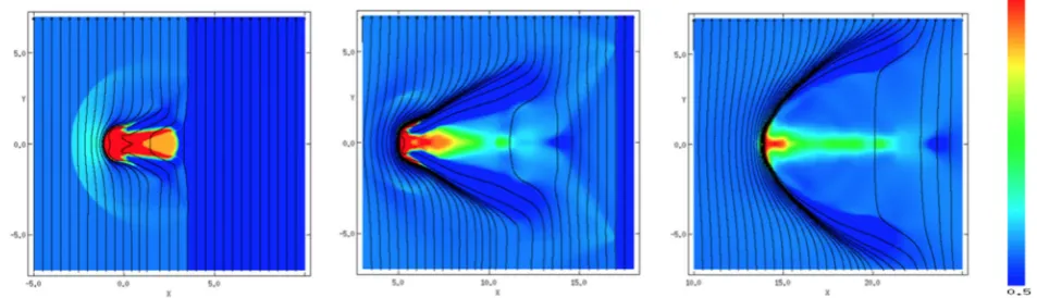
We first review the morphology of filaments embedded in an ini-tially parallel (i.e. at 0◦to the shock normal) magnetic field. Fig.5

presents snapshots of the time evolution of the density distribu-tion for simuladistribu-tionm10c1b1l4o45pa. The evolution of the filament broadly follows the stages outlined in section 4.1 of Pittard et al. (2009). First, the filament is struck and compressed by the shock front, and a bow shock is formed. Then the filament expands until

t≈6.46tcs. However, unlike the hydrodynamical spherical cloud case where the cloud broadly maintains its shape, the filament is

Table 2. A summary of the shock–filament simulations performed for a parallel magnetic field.Mis the sonic Mach number,χis the density contrast of the filament to the surrounding ambient medium,β0is the ratio of thermal to magnetic pressure,ldefines the length of the filament, andθdefines the angle

of orientation of the filament between its major-axis and the shock surface.vbis the shock speed through the inter-cloud medium (in code units).vpsis the

post-shock flow velocity, and is given in units ofvb.MAis the Alfv´enic Mach number,Mslow/fastare the slow/fast magnetosonic Mach numbers.tccis the

cloud-crushing time-scale of Klein et al. (1994), whiletcsis the cloud-crushing time-scale for a spherical cloud of equivalent mass introduced by Xu & Stone

(1995). Key filament time-scales are additionally noted. Values appended by†denote that the true value was greater than that given but that the simulation had ended before this point was reached.

Simulation M χ β0 l(rc) θ(◦) vb vps(vb) MA Mslow Mfast tcs/tcc tdrag/tcs tmix/tcs tlife/tcs

m10c1b1l2o45 10 10 1 2 45◦ 13.6 0.74 9.13 10.0 9.13 1.36 2.98 8.32 25.4

m10c1b1l4o45 10 10 1 4 45◦ 13.6 0.74 9.13 10.0 9.13 1.59 2.55 9.06 69.5

m10c1b1l8o45 10 10 1 8 45◦ 13.6 0.74 9.13 10.0 9.13 1.91 2.36 8.86 37.4

m10c1b1l4o0 10 10 1 4 0◦ 13.6 0.74 9.13 10.0 9.13 1.59 1.27 7.10 91.1

m10c1b1l4o30 10 10 1 4 30◦ 13.6 0.74 9.13 10.0 9.13 1.59 1.90 10.4 104

m10c1b1l4o70 10 10 1 4 70◦ 13.6 0.74 9.13 10.0 9.13 1.59 3.19 7.10 20.7

m10c1b1l4o85 10 10 1 4 85◦ 13.6 0.74 9.13 10.0 9.13 1.59 2.56 6.46 19.1

m10c1b1l4o90 10 10 1 4 90◦ 13.6 0.74 9.13 10.0 9.13 1.59 2.56 6.11 19.1

m10c2b1l4o45 10 102 ₁ ₄ ₄₅◦ _13.6 _0.74 _9.13 _10.0 _9.13 _1.59 _4.35 _5.17 _11.7

m10c3b1l4o45 10 103 ₁ ₄ ₄₅◦ _13.6 _0.74 _9.13 _10.0 _9.13 _1.59 _4.72 _4.49 _7.30

m10c1b0.5l4o45 10 10 0.5 4 45◦ 13.6 0.74 6.45 10.0 6.46 1.59 2.55 35.7 79.1

m10c1b10l4o45 10 10 10 4 45◦ 13.6 0.74 28.9 28.9 10.0 1.59 2.55 7.42 19.1

m1.5c1b1l4o45 1.5 10 1 4 45◦ 2.04 0.42 1.37 1.50 1.37 1.59 2.26 127† 127†

m3c1b1l4o45 3 10 1 4 45◦ 4.07 0.67 2.74 3.00 2.74 1.59 2.70 212 213†

(6)

Figure 5. The time evolution of the logarithmic density, scaled with respect to the ambient density, for modelm10c1b1l4o45pa. The evolution proceeds left to right, top to bottom, witht=0.95tcs,t=3.54tcs,t=6.11tcs,t=9.06tcs,t=14.2tcs, andt=52.5tcs. Note the shift in thexaxis scale for the final two

panels. The initial magnetic field is parallel to the shock normal.

instead contorted out of shape and the expansion of the cloud is less evident. The filament is swept downstream in the ambient flow, showing very little fragmentation due to the parallel magnetic field but continually being stripped of material. The presence of parallel magnetic field lines means that, unlike the hydrodynamic case, the MHD filament exhibits little or no surface instabilities, ensuring that the filament core survives for a far longer time-scale than would oth-erwise be possible. MHD filaments in a parallel field do not tend to form long tails of cloud material, but instead a linear ‘void’ is created which comprises an area of low density and high magnetic pressure. In non-oblique filaments (henceforth known as ‘axisymmetric’ fila-ments), and in particular filaments orientated atθ=90◦, this region forms a very clear ‘flux rope’, but where the filament is angled to the shock front (‘oblique’ filaments) such a structure is less well de-fined because the contortion of the filament in the ambient flow is not symmetric.

Figs6and7show the density distribution at various times for sim-ulationsm10c1b1l4o90pa andm10c1b1l4o0pa, respectively. The orientation of these two filaments leads to many more interesting features than those seen with the obliquely orientated clouds. For the interaction in Fig.6the filament is struck end-first, while in Fig.7the filament is struck on its broadside. The initial filament structure in Fig.6, after it has been struck by the shock, is very similar to that of the other runs, since the mechanical energy of the shock is driving the interaction rather than the magnetic energy of the filament. Compressed filament material is seen to form a column or ‘flux rope’ behind the filament head but the level of com-pression is limited in comparison with the purely hydrodynamic case due to the magnetic field lines which surround the filament and resist compression by the converging flow. The post-shock flow is prevented from entering the flux rope by the build-up of

magnetic pressure in that area. The surface of the filament, by con-trast, shows shear instabilities (though damped because of the field) which serve to create ‘wings’ – areas either side of the filament where the material is being ablated and bent by the surrounding flow (see section 3.1.1. of Al¯uzas et al.2014). Although the level of instability is greater than in the cases where the filament was orien-tated obliquely, the filament nonetheless remains relatively coherent and does not fragment. Instead it undergoes continual ablation to the surrounding flow until no substantial mass remains. The fila-ment withl=4 andθ=85◦begins to follow this evolution, and an initial well-defined flux rope is formed. However, since the filament is oriented at a slight angle to the shock front the structures forming on the axis behind the filament are quickly destabilized and the evolution proceeds as in the obliquely orientated cases described above.

The filament in Fig.7also forms ‘wings’. However, since the shock front strikes the entire length of the filament, the wings are far more substantial and act to shield the far side of the fila-ment from the flow. Therefore, the column of compressed mate-rial forming the flux rope in this instance is much broader than in the previous case. The filament is then dragged downstream by the post-shock flow, becoming elongated before finally being destroyed.

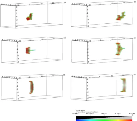
Fig.8shows a 3D volumetric rendering of the time evolution of the density of filament material in simulationsm10c1b1l4o45pa,

m10c1b1l4o90pa, and m10c1b1l4o0pa, showing clearly the flux rope associated with the filament orientated atθ =90◦, and also that material is forced out of the side of the filament in simulation

m10c1b1l4o45pa. Because only the filament material is shown, other features such as the bow shock are not displayed in these plots.

(7)

Figure 6. The time evolution of the logarithmic density, scaled with respect to the ambient density, for modelm10c1b1l4o90pa. The evolution proceeds left to right, top to bottom, witht=0.95tcs,t=3.54tcs,t=6.11tcs,t=9.06tcs,t=27.9tcs, andt=52.2tcs. Note the shift in thexaxis scale for the bottom two

Figure 7. The time evolution of the logarithmic density, scaled with respect to the ambient density, for modelm10c1b1l4o0pa. The evolution proceeds left to right, top to bottom, witht=0.95tcs,t=3.54tcs,t=6.11tcs,t=11.7tcs,t=27.9tcs, andt=52.2tcs. Note the shift in thexaxis scale for the bottom two

(8)

Figure 8. 3D volumetric renderings of modelsm10c1b1l4o45pa(top),m10c1b1l4o90pa(middle), andm10c1b1l4o0pa(bottom) att=3.54tcs (left-hand

column) andt=9.06tcs(right-hand column). The initial magnetic field is parallel to the shock normal.

0 0.2 0.4 0.6 0.8 1

0 20 40 60

(a)

mcore

(m

c

)

Time (tcs)

l2 l4 l8 spherical

0 20 40 60

(b)

Time (tcs) θ=0

θ=30

θ=45

θ=70

θ=85

θ=90

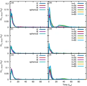
Figure 9. Time evolution of the core mass,mcore, for (a) a filament with variable length and an orientation of 45◦, and (b)l=4 with variable orientation, in

an initial parallel magnetic field.

3.1.2 Effect of filament length and orientation on the evolution of the core mass

In a purely hydrodynamical case with a Mach 10 shock the filament is destroyed within a short time-scale oft∼ 10tcs(the filament survives for longer when hit by a weaker shock – see Pittard &

Goldsmith2016). This is because turbulent instabilities are able to build up at the surface of the filament and encourage the ablation of mass from it. However, when magnetic fields are present instabili-ties are damped, and filaments survive over far longer time-scales. Fig.9shows the evolution of the filament core mass over time for

(9)

0 0.1 0.2 0.3 0.4 0.5 0.6 0.7 0.8

0 10 20 30

(a)

<v

x, cloud

(v

b

)

Time (tcs)

l2 l4 l8 spherical

0 10 20 30

(b)

Time (tcs) θ=0

θ=30

θ=45

θ=70

θ=85

θ=90

Figure 10. Time evolution of the filament mean velocity,vx, for (a) a filament with variable length and an orientation of 45◦, and (b)l=4 with variable orientation, in an initial parallel magnetic field. The dotted black line indicates the velocity of the post-shock flow.

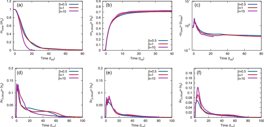
filaments with different lengths and orientations. It can be seen that the time-scale for destruction in these cases is far greater than in the hydrodynamical scenario presented in Pittard & Goldsmith (2016). We see that in terms of the core mass, the filament withl=4 and an orientation ofθ=90◦, and that with a length ofl=2 and an orientation ofθ=45◦, are destroyed att≈31tcsandt≈28tcs, respectively. However, the filament withl=4 andθ=0◦, and that withl=8 andθ = 45◦, are not destroyed untilt≈104tcs(not visible in the figure) andt≈61tcs, respectively.

The orientation of the filament to the shock normal plays an important role in the core mass evolution and the lifetime of the filament (Fig.9b). Whilst all filament orientations show a similar initial decrease in mass until t≈ 5tcs the filament orientated at θ =90◦(i.e. end on), although initially the slowest to lose mass, thereafter shows the most rapid drop in mass until its destruction (cf. fig. 28(i) in Pittard & Goldsmith (2016)). It is noticeable that those filaments with orientations of 0◦< θ45◦are much slower overall to lose the majority of their core mass (with the mass-loss rate decreasing significantly once less than 5 per cent of the initial filament mass remains), whilst those with orientations ofθ >45◦ are destroyed much more quickly.

Unless the filament is very short (in which case it begins to ap-proximate a spherical cloud), the length of the filament has less of an influence on the mass-loss than the orientation. From Fig.9(a) it can be seen that all three filaments initially show a similar decrease in their core mass. However, the filament with lengthl=2 subse-quently loses mass at a much faster rate than the other two lengths. This differs from the hydrodynamic case in Pittard & Goldsmith (2016), where the filament of lengthl=8 loses mass faster than the other filaments. Interestingly, the spherical cloud, whilst incurring a faster mass-loss rate than the filament withl=2, begins to level off at∼7tcsand retains approximately one tenth of its initial mass by the end of the simulation. In this case, although the ‘length’ of the filament is short, it is axisymmetric to the shock front and behaves in a similar manner to the filament of lengthl=4 andθ=0◦.

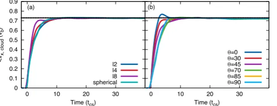
3.1.3 Effect of filament length and orientation on the mean velocity and the velocity dispersion

There are two stages to the acceleration of the filament through the ambient flow. The filament is first accelerated to the velocity of the transmitted shock,∝vb/√χ, as the shock is driven through it, and then further accelerated by the flow of post-shock gas until it reaches the velocity of the flow, e.g. 0.743vbforM=10,β0=1

and a parallel field. Fig.10shows the time evolution of the mean cloud velocity in thexdirection,vx. It can be seen that filaments

with orientations ofθ 45◦are initially accelerated faster than those with orientations ofθ >45◦, and this is likely to be because there is a greater surface area presented to the shock front with these orientations, i.e. the filament is ‘broadside’ to the shock front. It is interesting to note that the filament hit end on is initially accelerated the least rapidly, but that the rate of velocity gain does not level off as much as in some of the other models until the filament experiences a drastic reduction in acceleration atv0.6vb. It is clear that the

filaments withl=4 andθ=0◦, 90◦display more overtly the two-stepped nature of the acceleration. Att>40tcs, the filaments with θ=30◦andθ=90◦slightly overshoot and then decelerate to the velocity of the post-shock flow (not visible in Fig.10), possibly due to the release of some built-up tension in the field lines.

In comparison with the filament orientation, the length appears to have no significant effect on the mean velocity, with all filaments being accelerated at approximately the same rate. This is in contrast to the spherical cloud which displays a profile similar to the end on filament in Fig.10(b).

The interaction of shocks with filaments creates substantial ve-locity dispersions and reveals the presence of instabilities. In thex

direction, the filaments with orientationsθ70◦have the highest peaks (Fig.11d), with theθ=0◦andθ=30◦filaments showing the least dispersion in thexdirection. This is in agreement with Pittard & Goldsmith (2016) where, for end on or nearly end on filaments, theirδvx/vb also reaches 0.2 (cf. their fig. 28e). Figs11(e,f),

by contrast, indicate much less overall dispersion in theyandz directions. This is because, in thexdirection, the initial peak occurs as the transmitted shock travels through the filament. Thus, there is a large dispersion between the shocked and unshocked filament material at that time. A similar effect is produced in theyandz directions, although slightly later, when the filament is undergoing compression.

A comparison of the top and bottom panels of Fig.11reveals that the velocity dispersion is more sensitive to filament orientation than length in thexdirection, and more sensitive to length rather than orientation in thezdirection.

3.1.4 Effect of filament length and orientation on the mean density

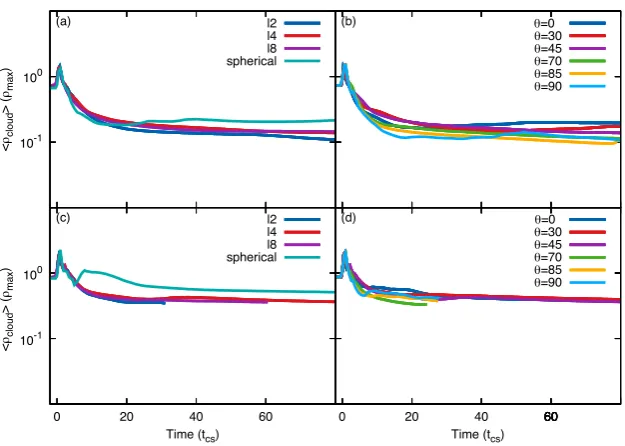
Fig.12shows the time evolution of the mean density of the fila-ment,ρcloud, and filament core,ρcore. The peak mean densities, after the shock has hit and compressed the filament, for various lengths and orientations of the filament are similar. However, the mean densities of filaments withl=4 andθ =90◦, orl=2 and θ=45◦, decline more rapidly, with a lower final value ofρ/ρmax being reached in these cases (though in Fig.12(d) the filament with

(10)

0 0.05 0.1 0.15

0.2 (a)

δ

vx, cloud

(v

b

)

l2 l4 l8 spherical

l2 l4 l8 spherical l2 l4 l8 spherical

(b) _θ₌₀

θ=30 θ=45 θ=70 θ=85 θ=90

θ=0 θ=30 θ=45 θ=70 θ=85 θ=90

θ=0 θ=30 θ=45 θ=70 θ=85 θ=90 0

0.05 0.1 0.15

(c)

δ

vy, cloud

(v

b

)

(d)

0 0.05 0.1 0.15

0 20 40 60 80

(e)

δ

vz, cloud

(v

b

)

Time (t_cs)

0 20 40 60 80

(f)

[image:10.595.142.455.55.364.2]

Time (t_cs)

Figure 11. Time evolution of the filament velocity dispersion in thex,y, andzdirections,δvx,y,z, for a filament with variable length and an orientation of 45◦ (left-hand column), andl=4 with variable orientation (right-hand column), struck by a parallel shock.

-1 0

10 10

-1 0

10 10

(a)

<

ρcloud

> (

ρmax

)

<

ρcloud

> (

ρmax

)

l2 l4 l8 spherical

(b) θ=0

θ=30 θ=45 θ=70 θ=85 θ=90

θ=0 θ=30 θ=45 θ=70 θ=85 θ=90

0 20 40 60

(c)

Time (tcs)

60 60 60 60 60

0 20 40 60

(d)

Time (tcs)

Figure 12. Time evolution of the mean density of the filament,ρcloud(top), and filament core,ρcore(bottom), normalized to the initial maximum filament

density, for filaments with (left-hand column) variable length and an orientation of 45◦, and (right-hand column)l=4 and a variable orientation, in a parallel magnetic field.

θ = 70◦ reaches a lower mean density level by the end of the simulation). It is noticeable in Fig.12(b) that for filaments with orientations ofθ=0◦,θ=30◦, orθ=90◦there is a subsequent increase in the mean density after reaching their lowest value, and this is mirrored in the spherical cloud mean density in Fig.12(a).

The initial peak of the spherical cloud mean density in Fig.12(c) is slightly higher than for the filaments, and a second, broader, peak is present also. The difference in the height of the peak mean densities may be due to the fact that the shocks driven into the filaments do not converge as well as those driven into the spherical cloud.

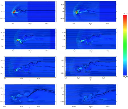
[image:10.595.142.455.403.626.2]

(11)

[image:11.595.70.520.56.438.2]

Figure 13. The time evolution of the logarithmic density, scaled with respect to the ambient density, for modelm10c2b1l4o45pa. The evolution proceeds left to right, top to bottom, witht=1.09tcs,t=1.97tcs,t=2.86tcs,t=3.65tcs,t=4.57tcs,t=5.36tcs,t=8.85tcs, andt=16.5tcs. Note the shift in thexaxis

scale for the final four panels, and the change in the logarithmic density scale compared to previous cases. The initial magnetic field is parallel to the shock normal.

3.1.5 χdependence of the filament evolution

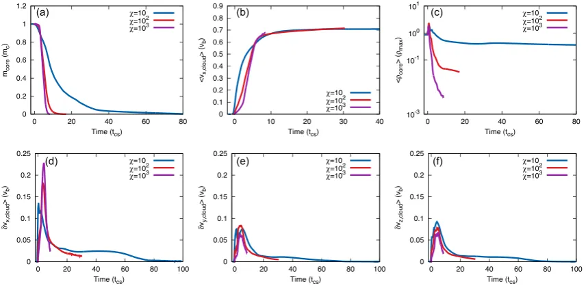
Varying the cloud density contrast radically alters the evolution of the filament. This is clearly seen in Figs13and14, where the filament downstream of the bow shock evolves in a highly turbulent manner, not dissimilar to previous hydrodynamical shock–cloud simulations (e.g. Pittard & Goldsmith2016). The tail of turbulent cloud material follows the pattern of the field lines at that point which are highly contorted and tangled. Since instabilities are able to form on the surface of the filament to a much greater degree than the other simulations run with a parallel magnetic field, the core mass of the filaments in these cases are destroyed in very short time-scales of t= 17.2tcsand t= 8.4tcs forχ = 100 and χ =1000, respectively, though they are first drawn out into long strands, or tails, of cloud material before being broken up into clumps and eventually mixed with the post-shock flow. Indeed, the development of turbulent instabilities increases with increasingχ. This is in complete contrast to theχ =10 case shown in Fig.5, where the evolving filament in that case forms a compact and smooth structure and does not display pronounced turbulent instabilities. The decreased destruction time of the filament (in units oftcs) with increasingχfollows the trend in Pittard & Goldsmith (2016), where

tlifereduces asχincreases whenM=10.2However, this is in direct contrast with Pittard & Parkin (2015), which revealed that spherical clouds do not show a clear trend withχ fortlifeatM=10. This shows thattmixand tlife do not exhibit monotonic behaviour with varyingχwhenM=10.

The demise of theχ =100 andχ=1000 filaments is seen in the mean density plot (Fig.15c), which shows that although these two filaments initially have a much higher mean density in com-parison withρamb, their mean density thereafter quickly reduces, while the filament withχ =10 maintains a much higher mean density after its initial compression by the shock front. In addition, Fig.15(b) shows that the filament withχ=1000 is destroyed be-fore it has reached the velocity of the post-shock flow. The presence of instabilities is, however, present in the velocity dispersion plots (Figs15d–f) with both the higherχfilaments producing a higher

2_{It should be noted that, owing to computational difficulties with running}

theχ=1000 simulation at such a high resolution, we used a slightly lower resolution ofR16for this case. Thus, it should be borne in mind that this

filament may be destroyed more rapidly than would be the case with a resolution ofR32.

(12)

[image:12.595.85.512.60.418.2]

Figure 14. The time evolution of the logarithmic density, scaled with respect to the ambient density, for modelm10c3b1l4o45pausing a resolution ofR16.

The evolution proceeds left to right, top to bottom, witht=0.33tcs,t=0.88tcs,t=1.43tcs,t=1.95tcs,t=2.50tcs,t=3.03tcs,t=3.57tcs, andt=4.11tcs.

Note the shift in thexaxis scale for the final three panels, and the change in the logarithmic density scale compared to previous cases. The initial magnetic field is parallel to the shock normal.

(a) (b) (c)

(d) (e) (f)

Figure 15. χdependence of the evolution for filaments withl=4 andθ=45◦. The initial magnetic field is parallel to the shock normal,M=10, andβ0=1.

Note that modelm10c3b1l4o45pawas run at a resolution ofR16.

[image:12.595.84.514.479.688.2]

(13)

(a) (b) (c)

[image:13.595.71.518.60.275.2]

(d) (e) (f)

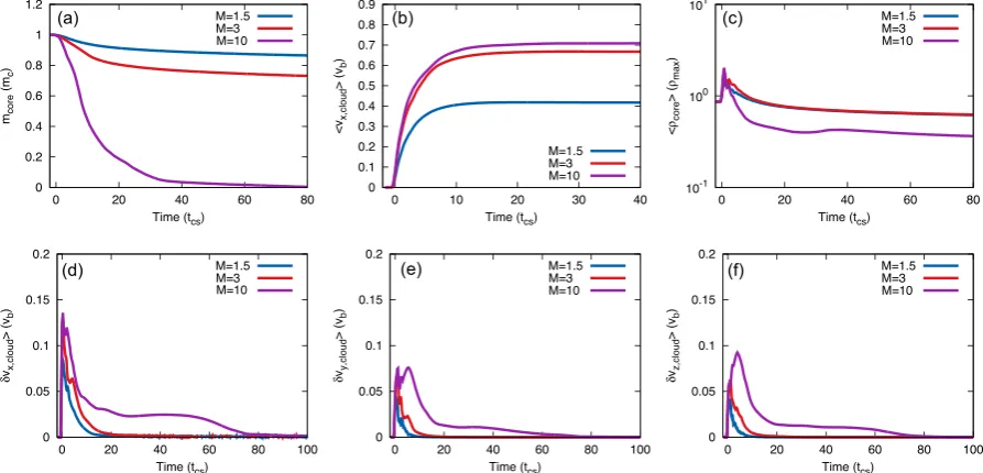
Figure 16. Mach number dependence of the evolution for filaments withl=4 andθ =45◦. The initial magnetic field is parallel to the shock normal, tχ=10, andβ0=1.

dispersion peak in thexdirection than theχ=10 filament. In addi-tion, the peak dispersion for higher values ofχis shifted from the χ=10 case in thexandydirections, indicating that turbulent insta-bilities take longer to form and are more important for the dispersal of the filament than its initial compression.

3.1.6 Mach dependence of the filament evolution

The Mach number of the shock can affect the growth rate of KH and RT instabilities, and can also affect the speed at which material is stripped from the filament and the time taken for the filament to become fully mixed with the surrounding flow. The post-shock conditions are dependent on the Mach number. In the purely hy-drodynamic case, low Mach numbers (i.e.M≤2.76 (Pittard et al.

2010)) lead to a subsonic post-shock flow with respect to a station-ary obstacle. Conversely, high Mach numbers provide a supersonic post-shock flow.

We investigated three values for the shock Mach number:

M=1.5, 3, and 10. Fig.16shows the Mach number dependence of the evolution. It is evident from Fig.16(a) that the core mass declines much more rapidly forM=10 than forM=1.5, indicating that core material exists for far longer with a low Mach number because of the milder interaction of the shock with the filament. The mor-phology of the filaments withM=1.5 andM=3 does not radically alter over time, with the filament merely being bent into a horse-shoe shape and experiencing very little compression or ablation of cloud material until the end of the simulation att=126.9tcs(for M=1.5) andt=212.7tcs(forM=3). It is clear, therefore, that the interaction of the shock with the cloud is much more gentle in these cases than forM=10. Fig.16(b) illustrates the differing values for the velocity of the post-shock flow according to Mach number, with very low Mach numbers resulting in a much slower acceleration to the (smaller) normalized velocity of the post-shock flow. The more gentle interaction at the lower Mach numbers results in the accel-eration of the filament up to the post-shock flow velocity while it is still intact and coherent in structure. In addition, a bow wave is formed ahead of the filament for shocks withM=1.5, rather than the bow shock visible forM=10 in Fig.5.

The velocity dispersion plots (Figs16d–f) show thatM=1.5 and

M=3 have a faster decay of velocity dispersions in all directions, in comparison toM = 10. Indeed, the difference in the height of the initial peak indicates that the filament has been struck by a shock of differing strength, since for the milder shocks there is far less of a contrast between the velocity of the shocked and unshocked portions of the filament when the shock front first hits the cloud.

3.1.7 β0dependence of the filament evolution

Fig.17shows the effect of varying the plasma beta on the evolution of the filament. Fig.17(a) shows that the core mass of the model with β0=10 (i.e. a weak magnetic field) is destroyed far quicker than for filaments with smaller values ofβ0(i.e. strong fields), since a weaker magnetic field is less able to damp the emergence of instabilities on the surface of the filament. The evolution withβ0=0.5 and β0=1 is, however, broadly the same, and the filament morphologies for these two cases are very similar, whereas that forβ0 = 10 shows far more fragmentation and dispersal of the cloud material. Figs17(b–f) show that there is not a great amount of divergence between the three simulations with respect to the filament velocity, mean density, or velocity dispersion in theydirection. However, the velocity dispersion in thexdirection does show some divergence at later times, once the structure and dynamics of the shocked filament become sensitive to the magnetic field strength, and the peak of the dispersion in thez direction increases with decreasing field strength.

3.2 Perpendicular field

3.2.1 Filament morphology

The time evolution of the density distribution for simulation

m10c1b1l4o45peis presented in Fig.18, with the magnetic field-lines visible in thexyplane in Fig.19. The presence of the perpen-dicular (i.e. 90◦ to the shock normal) magnetic field lines helps to protect the filament from the effects of the shock front and

(14)

(a) (b) (c)

[image:14.595.74.521.60.275.2]

(d) (e) (f)

Figure 17. Plasma beta dependence of the evolution for filaments withl=4 andθ=45◦. The initial magnetic field is parallel to the shock normal,M=10, andχ=10.

Figure 18. The time evolution of the logarithmic density, scaled with respect to the ambient density, for modelm10c1b1l4o45pe(cf. the parallel field case in Fig.5). The evolution proceeds left to right, top to bottom, witht=0.95tcs,t=3.44tcs,t=6.36tcs,t=8.95tcs,t=14.5tcs, andt=52.1tcs. Note the shift in

thexaxis scale for the final two panels. The initial magnetic field is perpendicular to the shock normal.

subsequent post-shock flow. Here, the field lines bend around the filament, allowing the flow to move along them and shielding the filament from rapid mass-loss via ablation. In the filaments set at an initial angle to the shock front (the ‘oblique’ filaments), the fil-aments are drawn out into long tendrils and are swept downstream in the flow. These filaments lose very little mass until near the end of the simulation. A small linear void is formed downstream of the filament, but this is much smaller than the void created in the

parallel field scenario. As with the parallel field, oblique filaments do not form any significant linear structure along their axis because they are asymmetrical to the shock front. Compared to the parallel field case in Fig.5, we observe that the perpendicular field ensures that the filament maintains a higher density, and produces a more rapid initial acceleration of the filament downstream. The latter is caused by the release of the tension that builds up in the field lines as they re-straighten.

[image:14.595.70.528.316.593.2]

(15)

Figure 19. As per Fig.18but showing thexyplane and magnetic fieldlines. The evolution proceeds left to right witht=0.95tcs,t=3.44tcs, andt=6.36tcs.

[image:15.595.66.524.256.539.2]

Note the shift in thexaxis scale for the final panel.

thexaxis scale for the bottom two panels. The initial magnetic field is perpendicular to the shock normal.

Fig.20shows snapshots of the density distribution for simulation

m10c1b1l4o90pe, again with the fieldlines in thexyplane shown in Fig.21. In the parallel field case, a flux rope would be expected to form on the axis behind the filament. However, with a perpendicular magnetic field this is not observed. Instead, low density filament material forms a linear structure along the axis and, in line with the parallel field scenario’s flux rope, this structure persists for some time. As in the parallel field case, the filament with l= 4 and θ =85◦begins to form a similar structure to this filament but the symmetrical nature of the evolving filament is quickly destabilized. The density distribution for the filament in simulation

m10c1b1l4o0peis depicted in Figs22 and 23. The morphology

of this filament at early times (i.e.t=3.54tcs) is very similar to that with a parallel field, except that the wings of this filament are swept backwards into the flow. From an observational point of view it may appear as if the filament has been struck by a shock travel-ling towards the−xdirection, and this may render the observational interpretation of such structures problematic. The beginnings of a very short, but broad, flux rope are present but this feature does not grow over time.

Fig.24shows a 3D volumetric rendering of the time evolution of the density of filament material in simulationsm10c1b1l4o45pe,

m10c1b1l4o90pe, andm10c1b1l4o0pe, clearly showing a ‘sheet-like’ structure at the upstream end of the filament. Because only the

(16)

[image:16.595.58.535.66.203.2]

thexaxis scale for the bottom two panels. The initial magnetic field is perpendicular to the shock normal.

filament material is shown, other features such as the bow shock are not displayed in these plots.

3.2.2 Effect of filament length and orientation on the evolution of the core mass

Amongst all the quantities being tracked, the reduction in the core filament mass shows the most dramatic difference between simula-tions with parallel and perpendicular magnetic fields. Fig.25shows the evolution of the core mass for filaments in a perpendicular field. The first point of note is that these filaments are very slow to lose their mass. Indeed, in all cases the filaments still comprised a sig-nificant amount of mass (between two and three fifths of the initial mass) byt=80t . This is in direct contrast to the filaments in a

parallel field. Whilst filaments withl=4 andθ=85◦and 90◦lose their mass more quickly (in agreement with the parallel field cases) it is interesting that the filament withl=4 andθ=0◦has lost the most mass byt=80tcs: in the parallel field simulations it was one of the filaments which conserved their mass the longest.

Considering Fig.25(a), the length of the filament does not appear to have a large influence over the evolution of the core mass, since all three filaments lose mass at approximately the same rate. The spherical cloud, in comparison, loses mass much more quickly, having lost approximately three fifths of its initial mass by the end of the simulation, as opposed to the two fifths that the other filaments have lost. Similar to the parallel magnetic field case, where the spherical cloud evolved in a similar manner to the filaments with θ=0◦, the spherical cloud in this case evolves in a similar manner to the filament withθ=90◦.

[image:16.595.74.521.247.524.2]

(17)

[image:17.595.70.522.266.665.2]

Figure 24. 3D volumetric renderings of modelsm10c1b1l4o45pe(top),m10c1b1l4o90pe(middle), andm10c1b1l4o0pe(bottom) att=3.44tcs(left-hand

column) andt=8.95tcs(right-hand column). The initial magnetic field is perpendicular to the shock normal.

(18)

0

Time (t_cs) 0

0

l4 l8

0 0.2 0.4 0.6 0.8 1 1.2

0 20 40 60 0000 20 40 60

(a)

mcore

(m

c

)

l2

spherical

Time (t_cs_cs) θ

(b) θ=0

θ θ=30=45 θ=70 θ=85 θ=90

Figure 25. Time evolution of the core mass,mcore, for (a) a filament with variable length and an orientation of 45◦, and (b)l=4 with variable orientation, in

an initial perpendicular magnetic field.

0 0.1 0.2 0.3 0.4 0.5 0.6 0.7 0.8 0.9

0 10 20 30

(a)

<v

x, cloud

(v

b

)

Time (t_cs) l2 l4 l8 spherical

0 10 20 30

(b)

[image:18.595.163.442.213.320.2]

Time (t_cs) θ=0 θ=30 θ=45 θ=70 θ=85 θ=90

Figure 26. Time evolution of the filament mean velocity,vx, for (a) a filament with variable length and an orientation of 45◦, and (b)l=4 with variable orientation, in an initial perpendicular magnetic field. The dotted black line indicates the velocity of the post-shock flow.

3.2.3 Effect of filament length and orientation on the mean velocity and the velocity dispersion

The plots showing the mean filament velocity in thexdirection (Fig.26) reveal that the filaments in all cases are accelerated to the velocity of the post-shock flow more rapidly than those in a parallel magnetic field. We expect the acceleration to be faster due to (i) the increased magnetic pressure which builds up on the upstream side of the filament, and (ii) the ‘snapping back’ of the field lines due to the magnetic tension which builds up as the field is dragged around the filament. In contrast to Fig.10(b), the filament withl=4 and θ=30◦levels off after the initial acceleration, before accelerating again to reach the post-shock flow velocity. Additionally, the fila-ment withl=4 andθ=0◦overshoots, before asymptoting to the velocity of the post-shock flow.

The length of the filament has little effect on the mean velocity, with all three filaments initially accelerating at the same rate. How-ever, the filament withl=8 andθ=45◦exhibits the ‘levelling-off’ seen in plot (b), a feature not present in Fig.10(a). The spherical cloud continues to smoothly and rapidly accelerate without level-ling off and thus reaches the post-shock flow velocity earlier than the three filaments.

With regard to the velocity dispersion plots, the length of the cloud is shown to have even less of an influence on the evolu-tion of this parameter than in the case of a parallel field (com-pare Figs27a–c to Figs11 a–c). However, there is a clear split in Figs27(d,f) between those filaments which are more ‘end on’ to the shock front, and those which are more ‘broadside’ to it. As in the parallel field case, those filaments with orientations of θ >45◦ have a greater initial dispersion in the xand z direc-tions, whilst filaments of varying length have very similar velocity dispersions in all directions. In all the velocity dispersion plots the peak of the dispersions is lower than those with a parallel field, indicating that the section of filament closest to the shock

front has undergone less compression in the perpendicular field case.

3.2.4 Effect of filament length and orientation on the mean density

The mean density plots (Fig.28) for bothρcloudand ρcore, in terms of the filament orientation, show very little difference between the simulations. However, as in the parallel magnetic field case, the filaments with orientations greater thanθ=45◦have a slightly larger drop in mean density, overall. Plots (a) and (c) of Fig.28show almost no change in the mean density between the simulations while the spherical cloud reduces to a much lower mean density consistent with the filaments withθ=0◦, and 90◦, indicating that the filament length is not important for the evolution of the mean density.

3.2.5 χdependence of the filament evolution

The evolution of filaments in a perpendicular field with increasing cloud density contrasts is radically different to those in a parallel magnetic field. Fig.29 shows that the filament is drawn out into long, smooth, tendril-like shapes which persist for far longer than the filaments in the parallel case (cf. Fig.13), while the highly-turbulent features present with a parallel field are not in evidence. In addition, the magnetic fieldlines are increasingly stretched around the filament and bunched together, as seen in Fig.30. The higher the value ofχ, the more drawn-out the filament is along thexaxis. This is evident in Fig.31(a), where the filaments with higher values ofχ retain almost two fifths of their initial mass at the end of the simulation, though that withχ=1000 still has a faster mass-loss rate in agreement with the parallel field case. The mean velocity and mean density plots for both parallel and perpendicular fields are very similar. However, the velocity dispersion plots show some differences, with much less dispersion in thexandydirections in Figs31(d,e).