This is a repository copy of Depth-based Hypergraph Complexity Traces from Directed Line Graphs.
White Rose Research Online URL for this paper: http://eprints.whiterose.ac.uk/94346/
Version: Accepted Version
Article:
Bai, Lu, Escolano, Francisco and Hancock, Edwin R orcid.org/0000-0003-4496-2028 (2016) Depth-based Hypergraph Complexity Traces from Directed Line Graphs. Pattern Recognition. pp. 229-240. ISSN 0031-3203
https://doi.org/10.1016/j.patcog.2016.01.004
Reuse
Items deposited in White Rose Research Online are protected by copyright, with all rights reserved unless indicated otherwise. They may be downloaded and/or printed for private study, or other acts as permitted by national copyright laws. The publisher or other rights holders may allow further reproduction and re-use of the full text version. This is indicated by the licence information on the White Rose Research Online record for the item.
Takedown
If you consider content in White Rose Research Online to be in breach of UK law, please notify us by
Elsevier Editorial System(tm) for Pattern Recognition
Manuscript Draft
Manuscript Number: PR-D-15-01351
Title: Depth-based Hypergraph Complexity Traces from Directed Line Graphs
Article Type: Full Length Article
Keywords: Hypergraphs Directed Line Graphs Entropies
Centroid Vertex
Depth-based Complexity Traces
Corresponding Author: Mr. Lu Bai,
Corresponding Author's Institution: University of York
First Author: Lu Bai
Order of Authors: Lu Bai; Francisco Escolano; Edwin Hancock
Abstract: In this paper, we aim to characterize the structure of hypergraphs in terms of structural complexity measure.
Measuring the complexity of a hypergraph in a straightforward way tends to be elusive since the hyperedges of a hypergraph may exhibit varying relational orders. We thus transform a hypergraph into a line graph which not only accurately reflects the multiple relationships exhibited by the hyperedges but is also easier to manipulate for complexity analysis. To locate the dominant substructure within a line graph, we identify a centroid vertex by computing the minimum variance of its shortest path lengths. A family of centroid expansion subgraphs of the line graph is then derived from the centroid vertex. We compute the depth-based
complexity traces for the hypergraph by measuring either the directed or undirected entropies of its centroid expansion subgraphs. The resulting complexity traces provide a flexible framework that can be applied to both hypergraphs and graphs. We perform (hyper)graph classification in the principal component space of the complexity trace vectors.
Depth-based Hypergraph Complexity Traces from Directed Line Graphs
Lu Bai (1), Francisco Escolano (2), Edwin R. Hancock (3)
(1) School of Information, Central University of Finance and Economics, Beijing, China.
Email address: [email protected] and [email protected].
(2) Department of Computer Science and Artificial Intelligence, University of Alicante, Spain.
Email address: [email protected].
(3) Department of Computer Science, The University of York, York YO10 5DD, UK.
Email address: [email protected].
Lu Bai is supported by National Natural Science Foundation of China (Grant No. 61503422).
Francisco Escolano is supported by the project TIN2012-32839 of the Spanish Government.
Edwin R. Hancock is supported by a Royal Society Wolfson Research Merit Award.
We aim to characterize hypergraphs in terms of structural complexity measures.
Straightforwardly measuring the complexity of a hypergraph tends to be elusive.
We transform a hypergraph
into a line graph for measuring the complexities.
We compute depth-based
complexity traces for the hypergraph on line graphs.
The complexity traces provide a flexible framework for hypergraphs and graphs.
Depth-based Hypergraph Complexity Traces from Directed Line
Graphs
Lu Bai1∗, Francisco Escolano2∗∗, Edwin R. Hancock3
1
School of Information, Central University of Finance and Economics, Beijing, China.
2
Department of Computer Science and Artificial Intelligence, University of Alicante, Spain.
3
the Department of Computer Science, University of York, York, UK.
Abstract
In this paper, we aim to characterize the structure of hypergraphs in terms of structural complexity
measure. Measuring the complexity of a hypergraph in a straightforward way tends to be elusive
since the hyperedges of a hypergraph may exhibit varying relational orders. We thus transform a
hypergraph into a line graph which not only accurately reflects the multiple relationships exhibited
by the hyperedges but is also easier to manipulate for complexity analysis. To locate the dominant
substructure within a line graph, we identify a centroid vertex by computing the minimum variance
of its shortest path lengths. A family of centroid expansion subgraphs of the line graph is then
de-rived from the centroid vertex. We compute the depth-based complexity traces for the hypergraph
by measuring either the directed or undirected entropies of its centroid expansion subgraphs. The
resulting complexity traces provide a flexible framework that can be applied to both hypergraphs
and graphs. We perform (hyper)graph classification in the principal component space of the
com-plexity trace vectors. Experiments on (hyper)graph datasets abstracted from bioinformatics and
computer vision data demonstrate the effectiveness and efficiency of the complexity traces.
Keywords: Hypergraphs, Directed Line Graphs, Entropies, Centroid Vertex, Depth-based
Complexity Traces
∗Email address: [email protected] and [email protected]. ∗∗Email address: [email protected].
Email address: [email protected].
*Manuscript
1. Introduction
There has recently been an increasing interest in the use of hypergraph models for higher
order learning. A hypergraph is a generalization of a graph. Unlike the pairwise nature of edges
in a graph, hypergraph representations allow a hyperedge to encompass an arbitrary number of
vertices, and can hence capture multiple relationships among features.
Most existing methods attempt to approximate a hypergraph by an equivalent graph, and
ex-ploit existing graph based methods for learning higher order models. For instance, Agarwal et
al. [1] have performed hypergraph clustering by partitioning a weighted graph obtained by
trans-forming the original hypergraph using a weighted sum of hyperedges to form edges. Zhou et al.
[2], on the other hand, have presented a similar graph approximation method for hypergraphs by
normalizing the Laplacian matrix of the star expansion of a hypergraph. Wachman et al. [3] have
developed a hypergraph kernel by enumerating similar walks on two hypergraphs. Zass et al. [4]
and Duchenne et al. [5] have separately applied high-degree affinity arrays (i.e. tensors) to
for-mulate hypergraph matching problems using different cost functions. Both methods address the
matching process in an algebraic manner but become intractable to compute if the hyperedges are
not suitably sampled. Shashua et al. [6, 7] have performed visual clustering using tensors to
repre-sent uniform hypergraphs (i.e. those for which the hyperedges have identical cardinality) extracted
from images and videos. Their work has been complemented by He et al.’s [8] algorithm for
de-tecting number of clusters in a tensor-based framework. Similar methods include those described
in [9, 10, 11, 12, 13], in which tensors (uniform hypergraphs) are used to represent the multiple
relationships between objects.
One limitation of most existing methods for hypergraph characterization is that they are
usu-ally restricted to uniform structures and cannot be applied to hypergraphs with arbitrary relational
orders. To address this shortcoming, Ren et al. [14] have exploited a set of polynomial coefficients
obtained from the hypergraph Ihara zeta function for characterizing nonuniform hypergraphs.
Un-fortunately, the computation of the hypergraph Ihara coefficients tends to be computational
bur-densome.
anal-ysis by computing a depth-based complexity trace for a hypergraph. We have previously explored
this idea for ordinary graphs [32], but we have not shown how to extend the idea to hypergraphs.
Our idea is to transform a hypergraph into an equivalent directed line graph that accurately captures
the multiple relationship exhibited by the hypergraph. The complexity trace of a hypergraph can
thus be computed by measuring the information content of a family of expansion subgraphs that
are derived from the centroid vertex of its line graph. Specifically, we explore how to characterize
the layer expansion subgraphs using complexity measures as a function of depth.
1.1. Literature Review
Computing the entropy-based complexity of an undirected (sub)graph has attracted significant
attention due to its fundamental practical importance for network analysis [32]. In early work,
K¨orner [16] developed a classical undirected graph entropy which poses complexity
characteriza-tion as an optimizacharacteriza-tion problem. This approach is based on a probability distribucharacteriza-tion associated
with the vertices, and the complexity is the minimal cross entropy between the probability
distri-bution and the vertex packing polytype of the graph. Unfortunately, this entropy is not applicable
to more general unweigthed graphs. Mowshowitz [17], Rashevsky [18] and Trucco [19] have
each developed a Shannon entropy for a graph associated with the probability distribution derived
from different partitionings of the vertex set. Unfortunately, determining the partitioning requires
expansive computation, thus the entropy cannot be efficiently computed. To overcome the
short-comings for these classical graph entropies, Dehmer et al. [20, 21] have developed a novel means
of computing entropies of undirected graphs by using information functionals. The information
functionals for an undirected graph are derived from the topological structure of the graph and
quantify the information content of the given graph structure. Moreover, this approach avoids the
combinatorial computations over different vertex partitions by constructing local information
sub-graphs for a given undirected graph, and thus achieves a polynomial time complexity. Anand et
al. [23] and Passerini et al. [22] have applied the von Neumann entropy (or quantum entropy) to
the domain of graphs through a mapping between discrete Laplacians and quantum states [24]. If
the discrete Laplacian [25] is scaled by the inverse of the volume of the graph we obtain a density
mea-sure distinguishes between different structures. For instance it is maximal for random undirected
graphs, minimal for complete ones and takes on intermediate values for star graphs. In addition,
when there is degree heterogeneity then the Shannon (classical) and von Neumann (quantum
in-formation theoretic) entropies are correlated. However, since the von Neumann entropy relies on
the computation of the normalized Laplacian spectrum, its computational complexity is cubic in
the number of vertices.
To render the computation of the von Neumann entropy more efficient, Han et al. [26] have
shown how the computation can be rendered quadratic in the number of the vertices by
approx-imating the Shannon entropy on the Laplacian eigenvalues using its quadratic counterpart. An
analysis of the quadratic entropy reveals that it can be computed from a number of permutation
invariant matrix trace expressions. This leads to a simple expression for the approximate entropy
in terms of the degrees of the adjacent vertices. Furthermore, to develop this work further, Ye
et al. [28] have shown how the von Neumann entropy for undirected graphs can be extended to
directed graphs. To do this, they commenced by using Chung’s [29] definition of the normalized
Laplacian on a directed graph. According to this definition, the directed graph normalized
Lapla-cian is Hermitian, and so the interpretation of Passerini et al. in [23] still holds for the domain of
directed graphs. The von Neumann entropy is essentially the Shannon entropy associated with the
normalized Laplacian eigenvalues. The resulting von Neumann entropy expression for directed
line graphs depends on the in-degree and out-degree of pairs of vertices connected by edges.
Recently, depth-based representations of undirected graph structures have been widely used
for developing new complexity measures for graphs [30, 31]. One approach is to gauge
informa-tion content flow through K-layer subgraphs of a graph (e.g. subgraphs around a vertex having a
maximum topological distance or minimal path length K) of increasing size and to use the flow
as a structural signature. Following this approach, Bai and Hancock [32, 33, 34] have developed
a fast depth-based complexity trace from the centroid vertex that has the minimum variance of
shortest path lengths to the remaining vertices (i.e., a depth-based representation around the
cen-troid vertex). They decompose a graph into a family of K-layer centroid expansion subgraphs
around the centroid vertex. A complexity trace vector is computed by measuring the entropies on
compute the entropy based complexity measures on a small set of expansion subgraphs rooted at
the centroid vertex, it can be thus computed in a polynomial time. By contrast, the thermodynamic
depth complexity measure developed in [30] requires the expansion subgraphs rooted at each
ver-tex, and computes the intrinsic complexity for each subgraph. It is thus less efficient to compute
on large graphs, e.g., a graph having thousands of vertices.
Unfortunately, all of the above mentioned complexity measures, both entropy-based and
depth-based, are only developed for (un)directed graphs and do not easily accommodate hypergraphs.
The reason for this is that straightforwardly measuring the complexity of a hypergraph tends to
be an elusive problem since the hyperedge in a hypergraph may exhibit varying relational orders.
Therefore, to measure the complexity of a hypergraph, in a manner that can precisely capture the
structural information contained within it, we consider transforming a hypergraph into a directed
line graph using the Perron-Frobenius operator [14]. The Perron-Frobenius operator can
repre-sent both uniform or nonuniform hypergraphs characteristics and can also accurately reflect the
multiple relationships exhibited by hyperedges of different orders. Hence, the directed line graph
representation for a hypergraph provides a convenient framework for complexity analysis.
1.2. Contributions
As previously stated, the aim of this paper is to present a novel framework for characterizing
hypergraphs based on computing depth-based complexity traces. Our starting point is the line
graph obtained by transforming a hypergraph into substructures using the Perron-Frobenius
op-erator. The complexity of the hypergraph is then measured by computing the entropies of the
substructures. We develop two different classes of complexity traces for a hypergraphHGbased
on two different decomposition strategies. The first is to establish an undirected line graphGU of
HGfrom the equivalent directed line graphGDLby simply neglecting the edge directions ofGDL.
We derive a family of expansion subgraphs with increasing layer sizeK fromGU. We construct
an undirected complexity trace ofHGby measuring how the undirected entropy measure varies
on the expansion subgraphs with increasingK. The second strategy is to establish a directed
com-plexity trace forHGby measuring the directed graph entropy on a family of expansion subgraphs
expansion subgraphs, both methods are efficient and overcome the computational bottlenecks
ex-isting in state-of-the-art methods for network complexity analysis [26, 30]. Our hypergraph
com-plexity traces provide a flexible framework that can be applied to both hypergraphs and graphs.
We perform experiments on several bioinformatics and computer vision datasets. We empirically
demonstrate that our complexity traces not only readily accommodate nonuniform hypergraphs,
but also easily scale to large hypergraphs. The performance of our framework is competitive with
alternative network complexity analysis methods and other hypergraph based methods reported in
the literature.
The remainder of this paper is organized as follows: Section 2 and Section 3 respectively
in-troduce the entropy measures for undirected or directed graphs that will be used in our framework.
For an undirected graph, Section 4 presents a family of centroid expansion subgraph that will
also be used in our framework. Section 5 describes how to compute an undirected or a directed
depth-based complexity trace for a hypergraph. Section 6 provides experimental comparisons
be-tween the proposed hypergraph complexity trace methods and state-of-the-art (hyper)graph based
methods. Section 7 concludes this work and makes suggestions for future work.
2. Entropy Measures on Undirected Graphs
In this section, we review how to compute the entropy for an undirected graph. We commence
by reviewing the concept of von Neumann entropy used in previous work [26]. Here we commence
by explaining how the von Neumann entropy of an undirected graph can be efficiently computed
in terms of the degree statistics using a quadratic approximation to the Shannon entropy. We
also introduce an alternative Shannon entropy using the probability distribution associated with a
steady state random walk on an undirected graph [32, 35].
2.1. Von Neumann Entropy of Undirected Graphs
The von Neumann entropy of an undirected graph is the Shannon entropy associated with the
eigenvalues of the normalized undirected graph Laplacian [22]. We denote the undirected graph
edges. The symmetric adjacency matrixAforG(V, E)is a|V| × |V|matrix that has elements
A(i, j) =
1 if(vi, vj)∈E;
0 otherwise.
(1)
The vertex degree matrix of G(V, E) is a diagonal matrix D whose elements are given by
D(vi, vi) = d(i) = Pvj∈V A(i, j). From the degree matrix and the adjacency matrix we can
construct the Laplacian matrix L = D − A. The normalized Laplacian matrix is given by
ˆ
L=D−1/2LD−1/2. The spectral decomposition of the normalized Laplacian matrix isLˆ = ˆΦˆΛ ˆΦT
where Λ =ˆ diag(ˆλ1,λˆ2, ...,λ|ˆV|) is a diagonal matrix with the ordered eigenvalues as elements
(0 = ˆλ1 <λˆ2 < ... <λ|ˆV|)andΦ = ( ˆˆ φ1|φˆ2|...|φ|ˆV|)is a matrix with the corresponding ordered
or-thonormal eigenvectors as columns. The normalized Laplacian matrix is positive semi-definite and
so has all eigenvalues non-negative. The number of zero eigenvalues is the number of connected
components in G(V, E). The von Neumann entropy of G(V, E)associated with the normalized
Laplacian eigenspectrum [22] is defined as
HV N =−
|V|
X
i=1
ˆ
λi
|V|log
ˆ
λi
|V| (2)
The computation of the von Neumann entropy requires a number of operations that is cubic
in the number of vertices |V|, since it requires the solution of the eigendecomposition. Han et
al. [26] have shown how the computation can be computed in quadratic time by a) approximating
the Shannon entropy by its quadratic counterpart, and b) evaluating the traces ofLˆ andLˆ2 using
vertex degrees. To commence, they approximate the Shannon entropy ˆλi
|V|ln ˆ
λi
|V| by its quadratic
counterpart λˆi |V|(1−
ˆ
λi
|V|)and obtain
HV N =−
|V|
X
i=1
ˆ
λi
|V|log
ˆ
λi
|V| ≃ |V|
X
i=1
ˆ
λi
|V|(1−
ˆ
λi
|V|)
= 1
|V|
|V|
X
i=1
ˆ
λi−
1 |V|2
|V|
X
i=1
ˆ
λ2i. (3)
Based on the definition by Han et al. in [26],P|V|
i=1λˆi =T r[ ˆL] = |V|, and P|V|
i=1ˆλ2i =T r[ ˆL2] =
|V|+P
(vi,vj)∈E 1
d(i)d(j). Thus, the von Neumann entropy defined in Eq.(3) can be re-written as
HV N(G) = 1−
1 |V|−
1 |V|2
X
(vi,vj)∈E
1
As a result, we can approximate the von Neumann entropy using two measures of an undirected
graph structure. The first is the number of vertices, and the second is based on degree statistics
for pairs of vertices connected by edges. The approximation bypasses calculating the normalized
Laplacian eigenvalues of an undirected graph which is (O(|V|3)). Therefore, we estimate the von
Neumann entropy in timeO(|V|2), and this renders the computation more efficient.
2.2. Shannon Entropy of Undirected Graphs
An alternative approach to computing the entropy of G(V, E)is to use a steady state random
walk onG(V, E). The probability of the steady state random walk onG(V, E)visiting vertexviis
P(i) =d(i)/X
vj∈V
d(j). (5)
Based on Eq.(5), we obtain a probability distributionP associated with the steady state random
walk onG(V, E), and the Shannon entropy forG(V, E)is given by
HS(G) =−
|V|
X
i=1
P(i) logP(i). (6)
For the undirected graphG(V, E), computing the Shannon entropyHS(G)requiresO(|V|2)
operations, because it needs to visit all the|V|2pairs of entries inAto compute the probability of a
steady state random walk visiting each vertex. This indicates that the Shannon entropy associated
with a steady state random walk can be efficiently computed.
3. Entropy Measures on Directed Graphs
The entropy measures defined in Section 2 only apply to graphs with undirected edges.
How-ever, in our study, we also require entropy measures on graphs with directed edges (see Section
5.3 for details). In this section, we introduce two entropy measures for directed graphs. We
com-mence by introducing a directed von Neumann entropy [28]. This method is based on extending
the definition of the von Neumann entropy (i.e., the von Neumann entropy of undirected graphs
defined in Section 2) from undirected to directed graphs, and is expressed in terms of the in-degree
and out-degree statistics of vertices. Moreover, we also introduce an asymptotic entropy in terms
3.1. Von Neumann Entropy of Directed Graphs
LetGD(VD, ED)is a directed graph with vertex setVD and edge setED ⊆VD ×VD, andAD
is the adjacency matrix ofGD. The in-degree and out-degree of vertexvD;i are
din(i) =
|VD| X
j=1
AD(j, i), dout(j) =
|VD| X
j=1
AD(i, j). (7)
With these ingredients, the transition matrixT for the directed graphGD is defined as
T(i, j) =
AD(i,j)
dout(i) if(vD;i, vD;j)∈ED
0 otherwise.
(8)
In [29], Cheng has shown that the normalized Laplacian matrix of a directed graph can be written
as
˜
LD =I−
Φ1D/2TΦ−D1/2+ Φ−D1/2TTΦ1/2
D
2 , (9)
whereΦD =diag(φD;1, φD;2, . . . , φD;|VD|)andφD = (φD;1|φD;2|. . .|φD;|VD|)is the left
eigenvec-tor ofL˜D.
Similar to the von Neumann entropy of an undirected graph [22], the von Neumann entropy
for a directed graph can also be approximated using the Shannon entropy associated with the
eigenvalues of its normalized Laplacian matrix. Using the approximation, in [28] Ye at al. have
extended the analysis of Han et al. [26] from undirected to directed graphs. The starting point
is the quadratic approximation to the von Neumann entropy in terms of the traces of normalized
Laplacian and the squared normalized Laplacian, i.e.,
HV ND = T r[ ˜LD] |VD| −
T r[ ˜L2
D]
|VD|2
. (10)
To simplify Eq.(10) one step further, letED;1andED;2are two disjoint subsets ofED, and satisfy
ED;1={(vD;i, vD;j)|(vD;i, vD;j)∈ED∧(vD;j, vD;i)∈/ED}andED;2 ={(vD;i, vD;j)|(vD;i, vD;j)∈
ED∧(vD;j, vD;i)∈ED}. ED;1SED;2 =ED, andED;1TED;2=∅. Based on [28], we have
T r[ ˜LD] =T r[I] =|VD|,
and
T r[ ˜L2
D] =|V|+
1 2(T r[T
2] +T r[TΦ−1
whereT r[T2] = X (vi,vj)∈ED;2
1
dout(i)dout(j)
andT r[TΦ−1TTΦ] = X
(vi,vj)∈ED
φ(i)
φ(i)dout(j)2
. Using
the fact that φD;i
φD;j ≈
din(i)
din(j) [28], we can approximate the von Neumann entropy of a directed graph
in terms of the in-degree and out-degree of the vertices as follows
HV ND = 1− 1 |VD|−
1 2|VD|2
X
(vi,vj)∈ED
1
dout(j)dout(i)
+ din(j)
din(i)dout(j)2
− X
(vi,vj)∈ED;1
1
dout(j)dout(i)
, (11)
or equivalently,
HV ND = 1− 1 |VD|−
1 2|VD|2
X
(vD;i,vD;j)∈ED
din(i)
din(j)dout(i)2
+ X
(vD;i,vD;j)∈ED;2
1
dout(i)dout(j)
. (12)
Eq.(11) or Eq.(12) can be consequently simplified according to the relative sizes of the sets
ED;1andED;2. IfGD is a weakly directed graph (|ED;1| ≪ |ED;2|), i.e., few of the edges are not
bidirectional, the approximate von Neumann entropy is defined as [28]
HW D
V N = 1−
1 |VD| −
1 2|VD|2
X
(vD;i,vD;j)∈ED
din(i)
dout(i) +
din(j)
dout(j) dout(i)din(j)
. (13)
On the other hand, ifGD is a strongly directed graph (|ED;2| ≪ |ED;1|), i.e., there are few
bidirec-tional edges, the approximate von Neumann entropy is given by [28]
HV NSD = 1− 1 |VD| −
1 2|VD|2
X
(vD;i,vD;j)∈ED
1
dout(i)din(j)
. (14)
Both the weakly and strongly directed forms of the von Neumann entropy (HW D
V N andHV NSD)
contain two terms. The first is the graph size while the second one depends on the in-degree
and out-degree statistics of each pair of vertices linked by an edge. Moreover, the computational
complexity of these expressions is quadratic in the graph size.
3.2. Asymptotic (Flow) Entropy of Directed Graphs
Heat kernels are the solutionK(β)to the heat/diffusion equation: ∂K∂β(β) =−LK(β), whereβ
SinceK(β)is semi-definite positive we have that the spectral decompositionK(β) = Ψe−βΛΨT
where Λ = diag(λ1, . . . , λ|V|) contains the eigenvalues 0 = λ1 < λ2 < . . . < λ|V| and Ψ =
(ψ1|ψ2|. . .|ψ|V|)the eigenvectors, leads to limβ→∞K(β) = ψ1ψ1T andψ1 = √1
|V|e, wheree
T is
the all ones row vector. Therefore, the latter limit is given the van der Waerden matrixB∗ = ee
T |V| .
An alternative way to formulate entropy is to quantify the amount of heat flowing through the
graph at a particular instant. Given an undirected graphG= (V, E)with unnormalized Laplacian
L = D −A, the amount of entropy is bounded by the maximum entropy of the Birkhoff-von
Neumann decomposition of the heat kernelK(β) =e−βL. This in ensured by thephase-transition
principledescribed in [30]: every graph is endowed with a phase-transition point corresponding
to the earlier instant where entropy is maximal. In addition, maximal entropy is achieved when
the maximum amount of heat is flowing through the graph.
Instantaneous heat flow as defined in [30] is given by the elements of the matrix product
F(β) = A : K(β), where X : Y = P
ijX(i, j)Y(i, j) is the Frobenius product. Hence, we
have thatF(∞) = A : K(∞) =A : B∗ = ||EV|| is associated with the asymptotic entropylog2(n)
of the Birkhoff decomposition for the kernel, and the asymptotic (flow) entropy of an undirected
graph is
HF =F(∞) = |
E|
|V|. (15)
The computational complexity of the asymptotic entropy is quadratic in the graph size, since it
needs to visit all the|V| × |V|entries of the adjacency matrix forG.
Given a directed graph GD(VD, ED), we assume that it it strong connected and aperiodic and
with transition matrixT given by Eq. 8. Otherwise,T is patched as in Pagerank [38] so that a left
eigenvectorφD.exists. The stationary distribution is given byPD(i) =φD;i. Then, following [29]
we have that the unnormalized directed LaplacianLD is defined as
LD = Φ1D/2L˜DΦ1D/2 = ΦD −
ΦDT +TTΦD
2 = ΦD −W . (16)
Since W(i, j) = (φD;iT(i, j) + φD;jT(j, i))/2, the role of the weight matrix W is to
sym-metrize LD by setting W(j, i) = 21φD;iT(i, j) = W(i, j) when dout(j) = 0, dout(i) > 0,
W(i, j) = 1
weighted adjacency matrix of an undirected graphGW = (VW, EW), where VW = VD, EW =
EDS{(i, j) : (j, i) ∈ ED} and the weights W(i, j) are associated to the edges. Thus, if the
original directed graph GD is strongly connected, then so is GW since the latter symmetrization
enables alternative paths between the vertices ofVD.
As a result, information diffusion constraints existing inGDare relaxed inGW. The constraints
are coupled to graph entropy through the phase-transition principle (the harder the constraints the
smaller the amount of heat flowing through the graph). The analysis of the heat kernel associated
with the directed LaplacianKD(β) =e−βLD =e−β(ΦD−W) entails the stationary distributionPD,
which is encoded in the diagonal ofΦD. More precisely, we have
KD(β) = e−β(ΦD−W)
= e−βΦD
I|VD|+βW+ β2
2!W
2+β3
3!W
3+. . .
≈
|VD|2 X
k=0 Wke
−βΦDβk
k! ,
(17)
andWkis defined in terms of walks of lengthk:
Wk(i, j) =X
Sk
k
Y
r=1
φD;irT(ir, ir+1) +T(ir+1, ir)φD;ir+1 2
, (18)
where Sk = {i1 i2 . . . ik+1} is a sequence of vertices defining a walk of length k. Therefore
Wk(i, j) is the sum of all walks of length k connecting i and j (see [39]). As a result of
sym-metrization, many of these walks acquire now non-zero probability. For instance, if(i, j) ∈ ED
but(j, i)6∈ED, there will be a directed path connecting verticesj andiinGD, since it is strongly
connected. However, in GW we will have W(j, i) > 0. Consequently, GW contributes with
many short links. The byproduct of a diffusion process is to create new links, called
transitiv-ity links. These links (j, i)do not exist in the original graph but are encoded in the components
of the heat kernelKDβ(j, i) > 0 as β increases. The spectral decomposition ofLD ensures that
limβ→∞KD(β) = B∗ = ee
T
|VD| as in the undirected case. However, since limβ→∞e
−βΦβk = 0for
the kernel will tend to n1 faster when they correspond to original directed edges. This means that
the asymptotic directed flowFD(∞) =AD :KD(∞) =AD :B∗ = ||EVDD|| is a good approximation
of the entropy trace even for moderate values of β. The reason for this is that it relies on the
density of the original directed graphGDwhose edges (and particularly their associated stationary
distribution) drive the diffusion process.
Hence, we have that the asymptotic (flow) entropy of a directed graph is
HF D =FD(∞) = |
ED|
|VD|
. (19)
The computational complexity of the asymptotic entropy is quadratic in the number of vertices in
the graphGD.
4. Centroid Expansion Subgraphs
In this section we define a set of centroid expansion subgraphs of an undirected graph. This set
will be used for establishing hypergraph complexity traces in Section 5. To commence, we identify
a centroid vertex and use this as the root vertex. To this end, for an undirected graphG(V, E), we
use Dijkstra’s algorithm to compute the shortest path matrixSGwhose elementSG(i, j)represents
the shortest path length between verticesvi andvj ofG(V, E). The average-shortest-path vector
SV for G(V, E) is a vector with the same vertex order as SG, and with each element SV(i) =
P|V|
j=1SG(i, j)/|V|representing the average shortest path from vertexvito the remaining vertices.
We identify the centroid vertexviforG(V, E)as follows
ˆ
vi = arg min
i
|V|
X
j=1
[SG(i, j)−SV(i)]2. (20)
The centroid vertexvˆi ofG(V, E)is located by selecting the vertex with the minimum variance
of shortest path lengths from all vertices inG(V, E). Therefore, the shortest paths starting from
the centroid vertexvˆi form asteadypath set that exhibits the least path length variance compared
with those path sets originating from the remaining vertices. The vertices surrounding the centroid
vertex in G(V, E) lie along different shortest paths from the centroid vertex, and the centroid
vertex has a global view of the vertex path length distribution surrounding it. LetNK
ˆ
ofV satisfying
NvˆKC ={u∈V |SG(ˆvC, u)≤K}. (21)
For a graphG(V, E)with the centroid vertexvˆC, theK-layer centroid expansion subgraphGK(VK;EK)
has the vertex setVK and edge setEK as follows
VK ={u∈NvKC};
EK ={(u, v)⊂NvKC |(u, v)∈E}.
(22)
The number of centroid expansion subgraphs is equal to the greatest length of the shortest path
from the centroid vertex to the remaining vertices of the graph.
5. Depth-based Complexity Traces of Hypergraphs
A hypergraph is usually denoted by a pair of setsHG(VH, EH)whereVH is a set of vertices
andEH is a set of non-empty subsets ofVH called hyperedges. To obtain hypergraph complexity
traces, we first establish a directed line graph using the Perron-Frobenius operator [40, 14]. The
reasons for using this graph representation for a hypergraph are twofold. First, pairwise-order
representations for hypergraphs allow the graph based complexity analysis to be applied to
hyper-graphs. Second, the directed line graph avoids the order ambiguities that arise from the
straight-forward expansion- or clique-based graph representations of a hypergraph [14]. Thus we develop
the complexity traces by computing the entropies of a family of centroid expansion subgraphs
obtained from the directed line graph.
5.1. Directed Line Graph
The directed line graph of a hypergraph is a dual representation in which each hyperedge is
rep-resented by a new vertex. For a hypergraphHG(VH, EH), the directed line graph GD(VD,−→ED)
can be established using Algorithm 1. Note that, for step 1 there are potential multiple edges
between two vertices in GH(VG, EG) if the two vertices are encompassed by more than one
common hyperedge in HG(VH, EH). Suppose there are p hyperedges encompassing two
ver-tices in HG(VH, EH). The p hyperedges inducep separated edges between the two vertices in
(a) A Hypergraph (b) Clique.
[image:19.612.83.521.61.454.2](c) Di-clique. (d) Directed Line Graph.
Figure 1: An example of transformation a hypergraph into a directed line graph.
G(V, E),−→ED is a set of directed edges of the directed graphGD(VD,−→ED). The adjacency matrix
TH ofGD(VD,−→ED) is the Perron-Frobenius operator of the original hypergraph. For the(i, j)th
entry ofTH, TH(i, j)is 1 if there is a simple edge directed from the vertexito the vertexjin the
directed line graph, and otherwise it is 0. Unlike the adjacency matrix of an undirected graph, the
Perron-Frobenius operator for a hypergraph is not a symmetric matrix. This is because the
con-straint in Eq.(24) arises in the construction of directed edges. Specifically, any two directed edges
induced by the same hyperedge in the original hypergraph are not allowed to establish a directed
edge in the directed line graph.
Algorithm 1:Establishing a directed line graph for a hypergraph
Input: A hypergraphHG(VH, EH)whereVH is a set of vertices, andE is a set of
non-empty subsets ofVH.
Output: A Perron-Frobenius operator ofHG(VH, EH)(i.e. the adjacency matrixTH of a
directed line graphGD(VD,−→ED)forHG(VH, EH)).
1: Establish the clique expansion graph forHG(VH, EH).
• Establish the clique expansion graphGH(VG, EG)forG(V, E)by connecting each pair of
vertices inei through an edge for each hyperedgeei ∈E, the vertex and edge sets are
VG =V;
EG ={(u, v)⊂ei |ei ∈E}.
(23)
2: Establish the associated symmetric digraph forGH(VG, EG).
• ForGH(VG, EG), establish the associated symmetric digraphDGH(VG, Ed)by replacing
each edge ofGH(VG, EG)by a directed edge pair in which the two directed edge are
inverse to each other.
3: Establish the directed line graph ofGH(VG, EG)throughDGH(VG, Ed).
• Establish the directed line graphGD(VD,−→ED)ofHG(VH, EH)based onDGH(VG, Ed).
The vertex setVD and edge set−→ED of theGD(VD,−→ED)are defined as
VD =Ed;
− →
ED ={(u, v)i,(v, w)j ∈Ed×Ed|i6=j}.
(24)
where the subscriptsiandj denote the indices of the hyperedges from which the directed
For the example hypergraph HG(VH, EH) shown in Fig.1(a), the clique graph GH(VG, EG) is
shown in Fig.1(b). InGH(VG, EG), the edges belonging to the common clique are indicated by
the same colour while the different cliques are coloured differently. Furthermore, there are two
different edges between v4 and v5, and these edges are induced by the hyperedge e3 and e4 of
HG(VH, EH), respectively. The associated symmetric digraph DGH(VG, Ed) of GH(VG, EG)
is shown in Fig.1(c), and the resulting directed line graph GD(VD,−→ED) from DGH(VG, Ed) is
shown in Fig.1(d).
The transformation of the hypergraphHG(VH, EH)into the directed line graphGD(VD,−→ED)
requires time complexityO(|VD|2). This is because the construction of the adjacency matrix of
GD(VD,−→ED)relies on visiting all the|VD|(|VD|=|Ed|) edges inDGH(VG, Ed)and establishing
all|VD|2 entries in the incidence matrix ofGD.
5.2. Theoretical Properties
The directed line graph and its Perron-Frobenius operator have several interesting properties.
a) Compared to the (hyper)graph adjacency or Laplacian matrix, the Perron-Frobenius operator
spans a higher dimensional feature space where it may expose richer (hyper)graph characteristics.
This property is a result of the fact that the cardinality of the vertex set for the directed line graph
is much greater than, or at least equal to, that of the original (hyper)graph. Hence, the adjacency
matrix (i.e. the Perron-Frobenius operator) of the directed line graph is described in a higher
dimensional space than the original (hyper)graph.
b)The directed line graph represents a (hyper)graph in a complete manner such that it naturally
avoids the information loss arising in the spectral truncation [10] or the clique graph approximation
[2]. This property is due to the constraint in Eq.(24), i.e., the connecting edge pair induced by the
same hyperedge in the original hypergraph cannot establish a directed edge in the directed line
graph. Actually this induces a bi-partition in the vertices ofVD. In other words, such a directed
line graph can distinguish different edges derived from the same hyperedge. This property is
illustrated in Fig.1(d). On the other hand, the clique expansion graph GH(VG, EG) from the
original hypergraphHG(VH, EH)only records adjacency relationships between vertex pairs of the
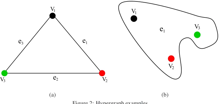
(a) (b) Figure 2: Hypergraph examples.
This property is illustrated in Fig.1(b). Hence, for two different hypergraphs (e.g., the hypergraphs
shown in Figs.2(a) and (b)) they may have the same clique expansion graph, and thus the same
resulted adjacency and Laplacian matrices resulting from the clique expansion graph. On the other
hand, the directed line graph defined in Eq.(24) may still produce total different structures for the
two hypergraphs. In Fig.2(b) we have an unique hyperedgee1that encodes the same clique which
defines the graph in Fig.2(a).
These properties indicate that the direct line graph and its Perron-Frobenius operator can offer
us an elegant way for hypergraph complexity analysis which can not only capture precise
hyper-graph complexity information but can also reflect richer characteristics of hyperhyper-graphs.
5.3. Depth-based Complexity Traces of Hypergraphs
We define a depth-based complexity trace for a hypergraph based on its directed line graph.
Simply establishing subgraphs with increasing layer size along the shortest paths on a directed line
graph tends to ignore certain topological information. The reason for this is that a path may not
exist between two given vertices in a connected directed line graph. To overcome this problem,
we identify the centroid vertex for the undirected line graph of a hypergraph. The undirected
line graph GU(VU, EU) of hypergraph HG(VH, EH) can be obtained by replacing each pair of
inversely directed edges inGDL(VDL,−→EDL)by an undirected edge. Then we develop two classes
of complexity traces forHG(VH, EH), which we refer to as the undirected complexity trace and
Definition 1 (Undirected complexity trace) For a hypergraphHG(VH, EH) and its undirected
line graphGU(VU, EU), the undirected complexity traceCTU is anLmaxdimensional vector
CTU = [H(G
U1),· · · , H(GUK),· · · , H(GULmax)]T. (25)
whereLmaxis the greatest length of the shortest paths from the centroid vertexvˆU
C to the remaining
vertices in GU(VU, EU), GUK is the K-layer centroid expansion subgraph of GU(VU, EU), and
H(GUK)is the entropy ofGUK. 2
Here the entropy function H(·) could be either the von Neumann entropy HV N(·) given in
Eq.(4) or the Shannon entropyHS(·)given in Eq.(6).
Next we describe how to extend these ideas to a directed complexity trace for the hypergraph
HG(VH, EH). For the directed line graph GDL(VDL,−→EDL) of HG(VH, EH), it is impossible
to establish a K-layer centroid expansion subgraph according to Eq.(22), because the edges of
GDL(VDL,−→EDL)are directed. For a hypergraphHG(VH, EH), given theK-layer centroid
expan-sion subgraphGUK(VUK;EUK)ofGU(VU, EU), we develop aK-layer pseudo centroid expansion
subgraphGDK(VDK;−E→DK)ofGDL(VDL,−→EDL)with vertex and edge sets as follows
VDK =VUK;
−→
EDK ={(u, v)∈−→ED |(u, v)∈ EUK}.
(26)
Note that there is a strict order for any pair of vertices(u, v)∈−E→DK.
Definition 2 (Directed complexity trace) For a hypergraph HG(VH, EH) together with its
di-rected line graphGDL(VDL,−→EDL)and undirected line graphGU(VU, EU), the directed complexity
traceCTD is anLmaxdimensional vector defined as
CTD = [HD(GD1),· · · , HD(GDK),· · · , HD(GDLmax)]T. (27)
where Lmax is the greatest length of the shortest paths from the centroid vertex ˆvU
C to the
re-maining vertices in GU(VU, EU), GDK is the K-layer pseudo centroid expansion subgraph of
GDL(VDL,−→EDL), andHD(GDK)is the entropy of the directed subgraphGDK. 2
Based on the definition in Section 5.1, the directed line graph of a (hyper)graph is a strongly
directed graph. Hence the entropy functionHD(·)should be the strongly directed von Neumann
entropyHD
Hypergraphs of Different Sizes: Note that, theLmax layer expansion subgraph is the undirected
line graph itself. The dimension of a hypergraph complexity trace vector is thus equal to the
greatest layerLmax. However, the complexity trace vectors for hypergraphs of different sizes may
exhibit various lengths. To compare these hypergraphs by using complexity trace vectors, we
need to make the vector lengths uniform. This is achieved by padding out the dimensions of the
complexity trace vectors. Hence, for complexity trace vectorsCTiandCTjof the two hypergraphs
HGiandHGj with dimensionsLpandLqrespectively, whereLp > Lq, we use theLq-th element
value ofCTj as the added padding value for the extendedLq+ 1-th toLp-th elements ofCTj.
5.4. Disscussions of the Hypergraph Complexity Traces
The two proposed depth-based complexity traces possess the following key features. a)Eq.(4)
indicates that the von Neumann entropyHV N is associated with the degrees of connected vertices.
Accordingly, the undirected complexity traceCTU is sensitive to changes of edge structures (e.g.
edge deletions) associated with vertices of low degrees inGU(VU, EU). Such edges usually form
bridges between vertex clusters inGU(VU, EU). Hence, the proposed undirected complexity trace
CTU associated with the von Neumann entropyHV N is sensitive to the interconnections between
vertex clusters withinGU(VU, EU). b)Eq.(6) indicates that for the Shannon entropyHS vertices
with large degrees dominate the value of the entropy. Hence, the undirected complexity trace
CTU associated with HS is suited to characterizing hypergraphs with strongly intra-connected
structures. c) Eq.(14) indicates that the von Neumann entropy HSD
V N depends on the in-degree
and out-degree statistics of each pair of vertices linked by an edge. Hence, the directed
com-plexity traceCTD associated withHSD
V N is sensitive to the in-degree and out-degree of each pair
of vertices connected withinGDL(VDL,−→EDL). d) As a result of the properties of a directed line
graph stated in Section 5.1, the proposed complexity traces from line graphs can reflect precisely
the rich complexity information for both uniform and nonuniform hypergraphs. e) Eq.(25) and
Eq.(27) indicate that the depth-based complexity traces provide a multi-dimensional complexity
characterization via the increasing layer substructures of the line graph from the centroid vertex.
Furthermore, since a hypergraph is a generalization of a graph and a graph can also be
special case of our hypergraph method. On the other hand, the complexity trace for a graph can
be directly constructed from the original graph by identifying its centroid vertex and establishing
the centroid expansion subgraphs on it (e.g., the depth-based complexity traces for graph defined
in [32]). However, the proposed complexity traces for a graph through its line graph can
cap-ture richer characteristics of complexity than those obtained from the original graph, because the
Perron-Frobenius operator can extract (hyper)graph characteristics in a higher dimensional feature
space than that of the original (hyper)graph. The proposed complexity traces for (hyper)graphs
fo-cus on measuring how the entropy based complexities of their subgraphs from the line graphs (i.e.
graphs transformed from the original (hyper)graphs) vary with increasing layer size. Such
com-plexity traces reflect high dimensional depth-based comcom-plexity characteristics of (hyper)graphs
and can be used for (hyper)graph clustering or classification. By contrast, the depth-based
com-plexity measure in [30], the Shannon entropy measures in [21] and the von-Neumann entropy
measure in [26] are based on the global structure of the original graph, and only provide an
uni-dimensional complexity characterization.
5.5. Analysis of Computational Complexity
Suppose the line graph, eitherGDL(VDL,−→EDL)orGU(VU, EU), extracted fromHG(VH, EH)
hasn vertices. The computational complexities for constructing the proposed complexity traces
forHG(VH, EH)are governed by the following processes. 1) The construction of the centroid
ex-pansion subgraphs which involves using Dijkstra algorithm to compute the shortest path matrix to
locate the centroid vertex and implementing the transformation from the hypergraphHG(VH, EH)
into the line graph. The Dijkstra algorithm takes timeO(n2). The transformation to the line graph
has time complexityO(n2). As a result the construction of the representation has time
complex-ity O(n2). 2) The computations of a) the von Neumann entropy in Eq.(4) and b) the Shannon
entropy in Eq.(6) for the centroid expansion subgraphs fromGU(VU, EU)(i.e., for the undirected
complexity trace), or c) the von Neumann entropy in Eq.(14) and d) the asymptotic (flow)
en-tropy in Eq.(19) for the centroid expansion subgraphs fromGDL(VDL,−→EDL)(i.e., for the directed
complexity trace). Through the definitions in Sections 2, 3 and 4, these entropies all require time
Lmax is equal to the greatest length of shortest paths from the centroid vertex ofG
U(VU, EU),
andLmax < n. Therefore, the worst-case time complexities of our undirected and directed
com-plexity traces forHG(VH, EH)using the four required entropies are allO(n3).
As a result, our depth-based complexity traces can be computed in polynomial time. The
reason for this is that we efficiently compute the required entropies on a small set of expansion
subgraphs rooted at the centroid vertex of a line graph. By contrast, the depth-based complexity
measure described in [30] establishes expansion subgraphs for each vertex of a given undirected
graph (e.g. a graph having n vertices) and then computes the intrinsic complexities on the
sub-graphs. It hence requires time complexityO(n7).
6. Experimental Evaluations
6.1. Hypergraph and Graph Datasets
We demonstrate the performance of our complexity traces on several (hyper)graph datasets.
We use a hypergraph based dataset abstracted from the COIL image database and five standard
graph based datasets abstracted from bioinformatics databases [30, 43, 44, 42] for the experimental
evaluations. These datasets are COIL (for hypergraphs), MUTAG, CATH1, CATH2 and PPIs (for
graphs).
COIL: The COIL database consists of images of 100 3D objects. In our experiments, we use
selected images for three similar cups, three similar bottles and three pieces of similar vegetables.
For each object we employ 18 images captured from different viewpoints. The hypergraphs are
abstracted using the feature hypergraph method [14]. Details about the feature hypergraph method
can be found in [14]. The maximum, minimum and average vertices of the COIL dataset are 549,
213 and 412.5 respectively.
MUTAG: The MUTAG dataset consists of graphs representing 188 chemical compounds. The
maximum, minimum and average number of vertices are 28, 10 and 17.93 respectively. The edges
of each compound are labeled with a real number, we transform these graphs into unweighted
graphs.
CATH1 and CATH2:The CATH1 dataset consists of proteins in the same class (i.e Mixed
proteins in the same class (i.e. Mixed Alpha-Beta), architecture (i.e. Alpha-Beta Barrel), and
topology (i.e. TIM Barrel), but in different homology classes (i.e. Aldolase vs. Glycosidases).
The CATH2 dataset is harder to classify, since proteins in the same topology class are structurally
similar. The protein graphs are10times larger in size than chemical compounds, with200−300
vertices. There are712and190testing graphs in the CATH1 and CATH2 datasets.
PPIs: The PPIs dataset consists of protein-protein interaction networks (PPIs). The graphs
de-scribe the interaction relationships between histidine kinase in different species of bacteria.
Histi-dine kinase is a key protein in the development of signal transduction. If two proteins have direct
(physical) or indirect (functional) association, they are connected by an edge. There are 219 PPIs
in this dataset and they are collected from 5 different kinds of bacteria. We select
Proteobacte-ria40 PPIs andAcidobacteria46 PPIs as the testing graphs. The maximum, minimum and average
number of vertices of the selected testing graphs are232,3and109.60respectively.
6.2. Evaluation of Interior Complexity Traces
We commence by illustrating the representational power of the proposed complexity traces
for hypergraphs. We demonstrate that they can be used to distinguish different hypergraphs. The
evaluation utilizes36hypergraphs abstracted separately from the images of two different objects,
namely a box and a cup in the COIL image database. For each object we use18images captured
from different viewpoints. The hypergraphs for individual images are established by using the
feature hypergraph method. For each hypergraph, we locate the centroid vertex of its (un)directed
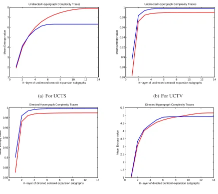
line graph, and construct the proposed complexity traces. Figs.3(a), (b), (c) and (d) show the
mean values of the undirected complexity traces using the Shannon entropy (UCTS) and the von
Neumann entropy (UCTV), together with the directed complexity traces using the von Neumann
entropy (DCTV) and the asymptotic (flow) entropy (DCTA), respectively. In Fig.3 the x-axis
represents the order of theK-layer centroid expansion subgraph for each hypergraph, while the
y-axis represents the mean entropy value as a function of the expansion subgraph order. Here the
blue and red lines represent the mean entropy values of the complexity traces for the hypergraphs
abstracted from the box and cup objects respectively. The main feature to note is that the mean
0 2 4 6 8 10 12 14 1 2 3 4 5 6 7 8
K−layer of undirected centroid expansion subgraphs
Mean Entropy value
Undirected Hypergraph Complexity Traces
(a) For UCTS
0 2 4 6 8 10 12 14
0.86 0.88 0.9 0.92 0.94 0.96 0.98 1
K−layer of undirected centroid expansion subgraphs
Mean Entropy value
Undirected Hypergraph Complexity Traces
(b) For UCTV
0 2 4 6 8 10 12 14
0.86 0.88 0.9 0.92 0.94 0.96 0.98 1
K−layer of directed centroid expansion subgraphs
Mean Entropy value
Directed Hypergraph Complexity Traces
(c) For DCTV
0 2 4 6 8 10 12 14
1 1.5 2 2.5 3 3.5 4 4.5 5 5.5
K−layer of directed centroid expansion subgraphs
Mean Entropy value
Directed Hypergraph Complexity Traces
[image:28.612.78.513.169.557.2]6.3. Experiments on Image Hypergraphs
6.3.1. Experimental setup
We illustrate the performance of our proposed complexity traces UCTS, UCTV, DCTV and
DCTA on a hypergraph classification problem. The hypergraph dataset for testing is again
ab-stracted from the COIL image database. We also compare our methods with several alternative
state-of-the-art hypergraph based learning methods. These methods include 1) the Ihara
coef-ficients for hypergraphs (HCIZF) [14], 2) the truncated Laplacian spectra (TLS) and truncated
normalized Laplacian spectra (TNLS) [2]. We compute the feature vectors of test hypergraphs
using both our own methods and the alternatives. We then perform 10-fold cross-validation using
the Support Vector Machine (SVM) Classifier associated with the Sequential Minimal
Optimiza-tion (SMO) [45] and the Pearson VII universal kernel (PUK) [46] to compute the classificaOptimiza-tion
accuracies. We use nine samples for training and one for testing. All the SMO-SVMs and their
parameters were performed and optimized on a Weka workbench [46]. To exclude random
ef-fects of fold assignments, we repeat the the whole experiments10times. We report the average
classification accuracy in Table I.
6.3.2. Experimental Results and Evaluations
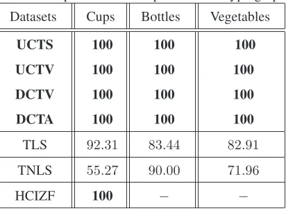
From Table 1 it is clear that our methods achieve the greatest accuracies over all image datasets.
1) Our UCTS, UCTV, DCTV and DCTA methods outperform TLS and TNLS which both use
spectral information for the hypergraphs. The reason for this is that our methods based on the
line graph of a (hyper)graph can capture richer (hyper)graph characteristics than the (hyper)graph
spectral representations. They also avoid the spectral truncation arising in TLS and TNLS.2)For
the hypergraphs extracted from the images of the cup object, the maximum and minimum number
of vertices are 310 and 213 respectively. Here the accuracy of HCIZF is competitive with that
of our complexity traces. Like our complexity traces, HCIZF also relies on directed line graphs,
and exploits richer (hyper)graph characteristics. However, for the hypergraphs extracted from the
images of the bottle and vegetable objects, where the maximum and minimum number of vertices
are 549 and 305 respectively, HCIZF is intractable for characterizing the hypergraph structures.
Table 1: Experimental Comparisons on Hypergraphs
Datasets Cups Bottles Vegetables
UCTS 100 100 100
UCTV 100 100 100
DCTV 100 100 100
DCTA 100 100 100
TLS 92.31 83.44 82.91
TNLS 55.27 90.00 71.96
HCIZF 100 − −
infinities even for hypergraphs of moderate sizes. In contrast, our proposed complexity traces can
easily scale to large hypergraphs, and our experimental results verify this advantage.
6.4. Experiments on Graphs
6.4.1. Experimental setup
We evaluate the performance of our proposed complexity traces UCTS, UCTV and DCTV
on a graph classification problem. The datasets for testing are abstracted from bioinformatics
databases. We also compare our methods with alternative state-of-the-art graph based learning
methods. The comparative methods include 1) the Weisfeiler-Lehman subtree kernel (WL) [47],
2) the von-Neumann thermodynamic depth complexity (VNTD) [30], 3) the von-Neumann graph
entropy (VNGE) [26], 4) the Shannon graph entropy (SGE) defined in Eq.(6), 5) the Shannon
entropies associated with the information functionals fV (FV) and fP (FP) [21], 6) the Ihara
coefficients for graphs (GCIZF) [14], and 7) the depth-based complexity traces of graphs [32]
computed using the Shannon entropy associated with both the steady state random walk (ECTS)
and the von Neumann entropy (ECTV). For the Weisfeiler-Lehman subtree kernel we compute
the kernel matrix of each dataset, and then perform Principle Component Analysis (PCA) on the
kernel matrix to embed graphs into a feature space. For the remaining methods, we calculate the
feature vectors or feature values of testing graphs. We then perform 10-fold cross-validation using
the SMO-SVMs described in Section 6.3 to compute the classification accuracies for each of the
methods in turn. We report the average classification accuracy over the 10-fold cross validation
evaluated under Matlab R2011a running on an Intel(i5) 2.5GHz 2-Core processor (i.e. i5-3210M).
6.4.2. Experimental Results and Evaluations
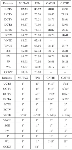
From Table 2, we can obtain the following conclusions. 1)On the MUTAG, CATH1 and PPIs
datasets, our complexity trace UCTS outperforms all the alternative methods. The complexity
traces UCTV, DCTV and DCTA outperform or are competitive to the alternative methods. On the
CATH2 dataset, our complexity trace UCTS outperforms all the alternative methods, excluding
the ECTV. The complexity traces UCTV, DCTV and DCTA outperform or are competitive to the
alternative methods. Key to the effectiveness of our methods is that our hypergraph complexity
traces probe a graph using the line graph, and can thus reflect richer graph characteristics in a
higher dimensional feature space. On the other hand, the alternative methods are based on the
original graph representation. In particular, the entropy based complexity measures (i.e. VNGE,
SGE, FV and FP) are simply computed based on the global structure of the original graph, and
only provide an uni-dimensional complexity characterisation. 2) Although GCIZF is also based
on a line graph representation, it is outperformed by our complexity trace methods on each of the
datasets studied. This is because the centroid expansion subgraphs allow our methods to capture
a depth-based information that GCIZF cannot convey. 3) The runtime of our complexity trace
methods is clearly faster than that of the alternative depth-based complexity method VNTD. It is
also competitive with GCIZF, the fast subtree kernel WL and the fast entropy measures VNGE,
SGE, FV and FP. The reason for this efficiency is that the required graph entropies in our methods
can all be computed in polynomial time. Compared to the depth-based graph complexity measure
VNTD, our complexity trace methods avoid either establishing the expansion subgraphs from
each vertex or computing the intrinsic complexities on the subgraphs. 4)Generally speaking, the
accuracies of our UCTS, UCTV and DCTV methods are very similar on the MUTAG, CATH1 and
CATH2 datasets. However, the accuracies of our UCTS method are obviously higher than those
of our UCTV and DCTV on the PPIs dadaset. The reason for this is that the entropy value of
an (un)directed graph computed using either the undirected or the directed von Neumann entropy
tends to be close to 1. This implies that the Shannon entropy is better suited for distinguishing
complexity traces with the entropies VNGE and SGE are obviously greater than those based on the
original entropies. This verifies again that our complexity trace methods capture richer structural
characteristics than the original graph based methods. 6) The accuracy of the DCTV method is
generally greater than that of the UCTV method, because DCTV considers directional information
residing on the edges of a line graph. However, UCTV ignores these edge directions. This also
implies that the performance of our complexity traces also depends on that of the required graph
entropy. Generally speaking, the hypergraph complexity traces computed using the Shannon or
von Neumann entropy (i.e., the UCTS or UCTV) outperform the graph complexity traces using the
same entropy (i.e., ECTS or ECTV). The reason for this is that the directed line graph obtained by
transforming the original graph can capture rich structural characteristics. This indicates that the
complexity traces from the line graph reflect deeper complexity information than those obtained
from the original graph. 7) Finally, for our DCTA method the accuracies on the MUTAG and
PPIs datasets are very good, but a little lower on the CATH1 and CATH2 datasets. The main
reason for this is that the edge density of the line graph is related to that of the original graph. The
graphs in the MUTAG and PPIs datasets are very sparse, with average edge density close to2.19.
However, for the CATH1 and CATH2 datasets, the average edge density is much larger, and is
about8.2. Since the required asymptotic (flow) complexity for the DCTA method is|ED|/|VD|,
the complexities for these (sub)graphs are thus similar. This indicates that the complexity measure
may not be suitable for graphs having high edge density, but perform well on sparse graphs.
7. Conclusion
In this paper, we have shown how to construct depth-based complexity traces for a hypergraph.
Our methods are based on transforming a hypergraph into a directed line graph. This not only
ac-curately reflects the multiple relationships exhibited by the hypergraph, but is also amenable to
complexity analysis. By neglecting the directed edges of the directed line graph, we have
identi-fied a centroid vertex, and thus obtained a family of expansion subgraphs around the vertex with
increasing layer size. The complexity traces of a hypergraph have been characterized by
measur-ing how the required entropies of these subgraphs vary with increasmeasur-ing layer size. Experiments
Table 2: Experimental Comparisons on Graphs
Datasets MUTAG PPIs CATH1 CATH2
UCTS 87.23 83.72 98.87 78.94
UCTV 86.17 75.58 98.45 77.89
DCTV 86.17 76.21 98.79 78.94
DCTA 86.17 79.09 92.13 72.63
ECTS 86.35 74.41 98.87 78.42
ECTV 84.57 70.93 98.73 80.47
VNTD 83.51 67.44 − −
VNGE 85.10 63.95 98.45 75.78
SGE 85.10 67.44 98.17 76.31
FV 84.57 70.93 96.76 76.31
FP 85.63 70.93 96.91 76.31
WL 84.57 73.25 98.17 73.15
GCIZF 80.85 70.93 − −
Datasets MUTAG PPIs CATH1 CATH2
UCTS 1” 45” 9′15” 6′12”
UCTV 1” 45” 9′15” 6′12”
DCTV 1” 53” 16′32” 10′50”
DCTA 1” 39” 8′55” 5′39”
ECTS 1” 1” 5” 2”
ECTV 1” 1” 5” 2”
VNTD 19′53” 49′50” >1day >1day
VNGE 1” 1” 1” 1”
SGE 1” 1” 1” 1”
FV 1” 1” 12” 5”
FP 1” 1” 12” 5”
WL 1” 1” 2′41” 51”
Our future plans are to extend the work in a number of ways. First, in prior work we have
developed methods for characterising graphs using the commute time [48] and the heat kernel
[49]. Both the commute time and the heat kernel of an undirected graph encapsulate the path
length information between vertices. It would be interesting to use the commute time or heat
kernel as a means of identifying a centroid vertex. Second, in [52] Haussler has proposed a generic
method, referred as R-convolution, to define a kernel between two graphs by decomposing them
and measuring the pairwise similarities between the resulting substructures. Examples include
graph kernels based on all pairs of a) walks [50], b) paths [51] and c) restricted subgraph or
subtree structures [47]. It would be interesting to use the expansion subgraphs defined in this paper
as a new type of depth-based (hyper)graph decomposition to define a novel (hyper)graph kernel.
Finally, in [53] we have explored the use of the discrete-time quantum walks on the directed line
graph, which can be constructed by transforming a hypergraph. It would be interesting to extend
this work, using the discrete-time quantum walks to compute the von Neumann entropy associated
with a quantum state. This may provide a more principled means of computing a quantum
depth-based complexity trace of a hypergraph.
Acknowledgments
This work is supported by National Natural Science Foundation of China (Grant No. 61503422).
Francisco Escolano is supported by the project TIN2012-32839 of the Spanish Government.
Ed-win R. Hancock is supported by a Royal Society Wolfson Research Merit Award.
References
[1] S. Agarwal, J. Lim, L. Zelnik-Manor, P. Perona, D. Kriegman, and S. Belongie, ”Beyond pairwise clustering,” in
Proceedings of IEEE Conference on Computer Vision and Pattern Recognition, 2005, pp. 838-845.
[2] D. Zhou, J. Huang, and B. Sch¨olkopf, ”Learning with hypergraphs: clustering, classification, and embedding,” in
Proceedings of Advanced Neural Information Processing System, 2007, pp. 1601-1608.
[3] G. Wachman, and R. Khardon, ”Learning from interpretations: a rooted kernel for ordered hypergraphs,” in
Proceedings of International Conference on Machine Learning, 2007, pp. 943-950.
[4] R. Zass, and A. Shashua, ”Probabilistic graph and hypergraph matching,” inProceedings of IEEE Conference on