Real-Time Temperature Estimation in a Multiple
Device Power Electronics System Subject
to Dynamic Cooling
Jonathan N. Davidson, David A. Stone, Martin P. Foster, and Daniel T. Gladwin
Abstract—This paper presents a technique to estimate the tem-perature of each power electronic device in a thermally coupled, multiple device system subject to dynamic cooling. Using a demon-strator system, the thermal transfer impedance between pairs of devices is determined in the frequency domain for a quantized range of active cooling levels using a technique based on pseu-dorandom binary sequences. The technique is illustrated by an application to the case temperatures of power devices. For each cooling level and pair of devices, a sixth-order digital IIR filter is produced, which can be used to directly estimate temperature from device input power. When the cooling level changes, the filters in use are substituted and the internal states of the old filters are converted for use in the new filter. Two methods for filter state con-version are developed—a computationally efficient method, which is suited to infrequent changes in power dissipation and cooling, and a more accurate method, which requires increased memory and processing capacity. Results show that the temperature can be estimated with low error using a system which is suitable for integration on an embedded processor.
Index Terms—Estimation, infinite impulse response (IIR) digi-tal filters, pseudonoise processes, temperature, thermal variables measurement.
I. INTRODUCTION
D
EMANDS on the thermal management of power convert-ers are increasing because of a strong industrial impetus for smaller, more efficient power electronics systems [1], [2]. Design engineers must, therefore, build systems using physi-cally smaller components with less heatsinking. However, the extent to which system designs can be miniaturized is limited by the rated maximum component temperatures, which may not be exceeded during normal operation. In addition, the life ex-pectancy of power converters is degraded by thermal cycling, where damage from multiple heating and cooling events ac-cumulates until system failure results [3]. A simple method of mitigation, often used in cheaper systems, is to incorporate large heatsinks and active cooling systems to maintain device temper-atures well below their rated maxima under all load conditions [4]. This solution suffers from two problems. First, the system and cooling must be sized for the worst-case condition, whichManuscript received September 3, 2014; revised April 30, 2015; accepted June 2, 2015. Date of publication June 9, 2015; date of current version November 30, 2015. This work was supported by the EPSRC under Grant EP/G037477/1. Recommended for publication by Associate Editor T. M. Lebey.
The authors are with the Department of Electronic and Electrical En-gineering, The University of Sheffield, Sheffield S1 3JD, U.K. (e-mail: [email protected]; [email protected]; m.p.foster@ sheffield.ac.uk; [email protected]).
Color versions of one or more of the figures in this paper are available online at http://ieeexplore.ieee.org.
Digital Object Identifier 10.1109/TPEL.2015.2443034
only occurs when the system is under full load (or fault con-ditions) in high ambient temperature conditions for prolonged operating periods. This is an unusual situation, however, and, under practical conditions, the system operates significantly below the worst case. The design for worst case leads to in-creased cost due to excess heatsink requirements and inin-creased energy usage in the active cooling system. Second, where active cooling is not controlled, temperatures rapidly increase and de-crease with system load, which can lead to significant thermal cycling [5].
In automotive applications, designing for thermal conditions below worst case is a reasonable approach if measures are taken to mitigate the risk from overheating semiconductor devices. Such measures include reducing the load and increasing cool-ing if the device temperatures would otherwise be exceeded. In electric vehicles, load reduction could be achieved by a tempo-rary lessening of wheel torque or speed, where a small reduction will have limited impact and the mechanism to achieve it can safely be incorporated into the vehicle management system for most categories of vehicle. To allow effective mitigation, a tech-nique to monitor the temperature of critical devices is required. While temperature sensors could provide the required informa-tion, they represent an additional per-unit cost to the system. Instead, in this paper, we propose a mathematical real-time tem-perature estimator based on the power dissipation in devices within the system. Additionally, the effect of variable cooling such as from a fan or blower is considered.
Early work on estimating and predicting the temperature of components under variable cooling used an analytical approach, such as that proposed by Fried [6]. This type of modeling is limited by the necessity to determine the physical parameters of the derived equations, which is especially difficult in cases where thermal cross coupling between devices is to be considered. In these cases, a numerical approach is preferable since complex parameters need not be determined. More recently, Lundquist and Carey [7] use an analytical model to predict the future temperature of a computer processor under a prospective level of forced air cooling. Together with direct measurement of the actual processor temperature, the technique is used to control the temperature at an optimal level. In this study, we eliminate the need for direct measurement in similar systems by implementing accurate temperature prediction.
Musallam and Johnson [8] propose using compact models be-tween each input–output pair in a thermal system with multiple points of interest. Using a combination of finite-element analy-sis (FEA) and direct experimental characterization, the thermal
transfer function between each input–output pair is calculated in the Laplace domain. From this data, a matrix is constructed that describes the relationship between every heat source in-put and every temperature-of-interest outin-put. By transforming the model into a discrete-time expression, a computationally efficient real-time temperature estimator is developed. Exper-imental validation confirms the accuracy of the estimations; however, the work is limited to thermally linear systems, where the transfer functions are unchanged throughout operation. The technique cannot, therefore, be used directly in a system with variable cooling.
A solution that overcomes this problem is proposed by James et al. [9], who consider the effect that variable forced-air cool-ing has on thermal dynamics. The authors propose that for a multiple device system, a series of thermal impedance matrices can be found, where each matrix describes the system dynam-ics at a given cooling level. However, for the system examined, it is found that the model can be simplified by neglecting the dependency of thermal cross coupling on the level of cooling, thus simplifying the mathematics. The authors identify this as a limitation of their approach. In the present paper, an extended approach that overcomes this simplification and explicitly con-siders the effect of cooling level on the thermal cross coupling is therefore proposed.
This paper reports a measurement-based characterization of the system. Alternatives to this approach include the offline mod-eling of a system using FEA and computational fluid dynamics [10]. Models developed from FEA can later be simplified and incorporated into a control system. The FEA approach is limited by the requirement for the model to precisely match the practi-cal system. In addition, numeripracti-cal modeling of turbulent flow is difficult [11]. It is shown by Rodgers et al. [12] that more prac-tical thermal analysis is preferable in many cases. In this paper, we therefore present an experiment-based characterization of a power electronic system under controlled cooling.
[image:2.594.311.556.499.638.2]Previously [13], we presented a method to estimate the tem-perature over several devices coupled on a heatsink by char-acterizing the cross coupling between them. In this paper, a similar technique is used wherein a pseudorandom binary se-quence (PRBS) power dissipation waveform is applied to each power device in turn, and the resulting temperature response at all devices is measured. Due to the special nature of the PRBS (which we will explore later in this paper), it is possi-ble to determine the cross coupling (i.e., the thermal transfer impedance) between each pair of devices over a band of fre-quencies. In this study, the cross coupling is used to estimate the temperature response to a given power input and cooling level using a novel technique that results in accurate estimation. The particular topology studied in this study concerns temper-ature estimations with an update rate of 1 Hz or less, and is, therefore, sensitive to temperature changes due to load, rather than individual switching events. To illustrate the technique, the study is applied to device case temperatures, although the pre-sented estimation techniques could equally be applied to the junction temperature following a junction-temperature-based characterization.
Fig. 1. Norton equivalent electrical circuit between heat dissipation pointx and temperature measurement pointy.
II. THERMALSYSTEMCHARACTERISATION
A. Cross Coupling
A linear thermal system can be represented by the thermal transfer impedance, or cross coupling, between its heat sources and points, where the temperature is to be measured. In a power electronics system, we are normally concerned with only the few points whose temperatures are limited by device physics and construction, and are likely to exceed rated levels. Typically, these are the electronic power devices that dissipate high power and are damaged by overheating. To model the thermal cross coupling, we consider the problem using Norton’s theorem and superposition theory. The relationship between each dissipating device and each temperature of interest is approximated using the equivalent electrical circuit in Fig. 1.
We useQxto denote the power dissipated at pointx,Θy for
the temperature at pointy andZth·x→y for the cross coupling
between pointsxandy. To simplify the mathematics, we use these quantities in the frequency domain, which we signify us-ing upper case symbols (lower case symbols are used for the time domain). From Ohm’s law and superposition theory, the temperature at any pointydue to the power dissipations at all points in the system can be expressed in matrix notation as in (1) and (2). It is possible to use simple point-by-point multipli-cation in these calculations because the mathematics is carried out in the frequency domain
Θ(jω) = Zth(jω)·Q(jω) (1)
Zth =
⎛ ⎜ ⎜ ⎜ ⎝
Zth·1→1 · · · Zth·n→1
..
. . .. ...
Zth·1→m · · · Zth·n→m
⎞ ⎟ ⎟ ⎟ ⎠; Θ=
⎛ ⎜ ⎜ ⎜ ⎝
Θ1
.. .
Θm
⎞ ⎟ ⎟ ⎟ ⎠
Q=
⎛ ⎜ ⎜ ⎜ ⎝
Q1
.. .
Qn
⎞ ⎟ ⎟ ⎟
⎠ (2)
where Θ(jω) andQ(jω)are column vectors of temperature and powers at each relevant point, respectively,Zth(jω)is the
matrix of every cross coupling impedance between each set of relevant points, andnandmare the number of power dissipation points and relevant temperatures, respectively.
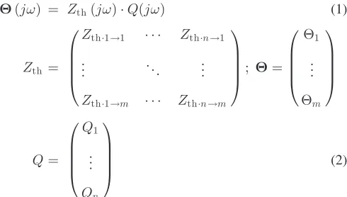
Fig. 2. Experimental arrangement.
Fig. 3. Frequency domain representation of an 8-bit maximum length PRBS signal clocked at 1 Hz. The response was calculated using the DFT.
active cooling from a blower with a controllable angular fre-quencyδ. To demonstrate the techniques presented in this paper, a test system of D2PAK devices mounted on an insulated metal substrate board is constructed. The power dissipation in each device is controlled by an external circuit. In order to perform the characterization measurements and to verify the tempera-ture estimations generated by the proposed technique, a K-type thermocouple is attached to the tab of each device to monitor the temperature. A speed-controlled blower is positioned to blow over all devices and an external computer controls and monitors all elements. The physical layout is shown in Fig. 2.
When active cooling is present, the cross-coupling matrixZth
is not only a function of frequency but is also a function of the level of active cooling – blower speed in this case. The matrix is, therefore, denoted asZth(jω, δ). Determining the elements
of this matrix over all blower speeds and frequencies produces a complete model of the system.
B. Generation of Cross-Coupling Characteristics using PRBSs
In previous work [13], [14], we have demonstrated that PRBS can be used to characterize the thermal cross coupling between devices. Using the same principles, the cross coupling is calcu-lated over a range of blower speeds in this study. The PRBS tech-nique is essentially a practical form of band-limited white noise system identification [15]. It uses a PRBS test signal, which has almost uniform frequency content over its bandwidth as shown in Fig. 3. For thermal analysis, the relationship between power and temperature under given operating conditions (e.g., cooling level, chemical phase of materials) is approximately lin-ear because heat transfer is a diffusion process described by a linear equation [8]. Therefore, when a PRBS power signal is ap-plied to the thermal system, the temperature response spectrum
reflects the system’s frequency response over the test signal’s bandwidth.
A PRBS signal is applied to each device in turn and the tem-perature responses between every pair of devices are measured using a thermocouple and logged by computer. This experiment is repeated over a range of blower speeds to fully character-ize the cross coupling. The cross-coupling thermal impedance
Zth·x→y between devicesxandyat any frequency and blower
speed can be calculated according to
Zth·x→y(jω, δ) =
Θy(jω, δ)
Qx(jω)
(3)
where Qx is ann-bit PRBS power signal applied to devicex
which, when clocked at frequencyωc, produces a valid
temper-ature responseΘy at deviceyover the bandwidth [14] in
ωc
2n −1 ≤ω≤
ωc
2.3. (4)
In this paper, a 9-bit (n= 9) PRBS is used clocked at 0.25 Hz, leading to a valid frequency response between 0.5 and 110 mHz. The experimental arrangement to perform the characterization is shown in Fig. 4. A microcontroller generates a PRBS voltage waveform (using the linear feedback shift register method with taps on the fifth and ninth registers to produce a maximum length sequence). This voltage controls a current source that determines the power dissipation in the D2PAK resistors through control of
I2Rlosses. The temperatures of the devices are measured using
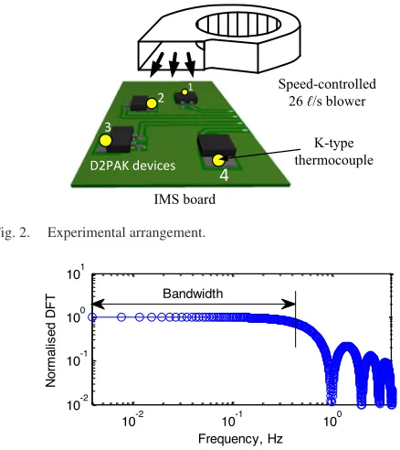
a thermocouple and both power input and temperature output are logged by computer. The characterization procedure is repeated at 22 blower speeds distributed with approximate logarithmic spacing in the range of 0 and 6600 revolutions per minute (rpm). Experiment control and data processing are handled by a PC running LABVIEW and MATLAB.
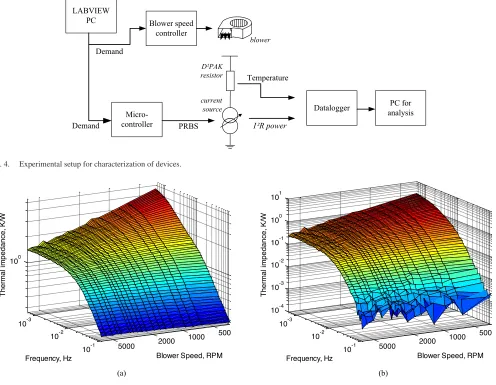
The results at each blower speed can be presented in a Bode plot. An extra dimension is added to the graph to show the effect of blower speed. Fig. 5, therefore, shows a three-dimensional (3-D) Bode plot of Zth·1→1(jω, δ) and Zth·3→1(jω, δ). The
Zth·3→1(jω, δ)plot shows increased noise at high frequency
due to the low-thermal impedance from cross-coupling char-acteristics. The effect is negligible because the temperature re-sponse of a system is determined mainly by the lower frequency region.
Fig. 4. Experimental setup for characterization of devices.
Fig. 5. Three-dimensional Bode plots of the autocoupling of device 1 over the available range of blower speeds and frequencies. Note that all axes are logarithmic. (a)Zt h·1→1. (b)Zt h·3→1.
III. ESTIMATION OF THETEMPERATURERESPONSE
A. Estimation Using the Cross-Coupling Frequency Response Directly
The temperature response measured at a single device due to dissipation in another device can be directly calculated in the frequency domain using
Θy(jω, δ) =Zth·x→y(jω, δ)·Qx(jω). (5)
This direct technique requires the input power waveform to be converted into the frequency domain and the response to be converted back into the time domain. These conversions can be achieved using the discrete Fourier transform (DFT): the required conversions to and from the frequency domain are given in (6) and (7), respectively,
θy(t) = F−1(Qx(jω)) (6)
Qx(jω) = F(qx(t)) (7)
whereF represents the DFT (F−1 is the inverse), andθandq
represent the time-domain temperature and power, respectively.
B. Representation of Cross Coupling as a Digital Filter
In [13], it has been shown that Fourier transforms are com-putationally intensive and require a significant number of math-ematical operations. To reduce the computational complexity, the model of the system is converted to a digital infinite impulse response (IIR) filter. Using a digital filter has the advantage of being computationally light since only a few real number cal-culations need be performed for each time sample. A digital filter is fitted to each element of the cross-coupling matrix us-ing the MATLAB function invfreqz, which finds filter vectors
aandb such thatZth in (8) is the best approximation to the
measured cross coupling [16]. This process effectively converts frequency-domainZth(jω)to a digital filter with the equivalent
transfer function in the z-domain,Zth(z). A different filter will
result for each level of active cooling and each pair of power input and temperature measurement points
Zth(z) =
H
λ= 0bλz−λ
1 +Gλ= 1aλz−λ; z=e
−j2π(ω
ω s) (8)
whereωsis the sampling frequency, andHandGare the
Fig. 6. Simple digital filter arrangement for temperature estimation with con-stant active cooling.
of the filter to an arbitrary input sequence can be calculated us-ing (9). This equation can also be expressed as the time-domain difference equations shown in (10) and (11) [17]. In this form, the input power at each time step can be evaluated individually, with the system state stored as a state vectors= (s0, . . . , sL−1),
whereLis the greater ofGandH(aλ= 0forλ> Gandbλ= 0
forλ> H). In this study,G= 3andH = 6are selected as
suit-able filter lengths since these are the smallest values produce accurate results
θ[i] =
G
λ= 1
aλθ[i−λ] +
H
λ= 0
bλq[i−λ] (9)
θ[i] = q[i]·b0+s0[i−1] (10)
s[i] =
⎛ ⎜ ⎜ ⎜ ⎜ ⎜ ⎜ ⎜ ⎝ s0 .. .
sL−2
sL−1 ⎞ ⎟ ⎟ ⎟ ⎟ ⎟ ⎟ ⎟ ⎠
[i] =q[i]·
⎛ ⎜ ⎜ ⎜ ⎜ ⎜ ⎜ ⎜ ⎝ b1 .. .
bL−1
bL ⎞ ⎟ ⎟ ⎟ ⎟ ⎟ ⎟ ⎟ ⎠ + ⎛ ⎜ ⎜ ⎜ ⎜ ⎜ ⎜ ⎜ ⎝ s1 .. .
sL−1
0 ⎞ ⎟ ⎟ ⎟ ⎟ ⎟ ⎟ ⎟ ⎠
[i−1]−θ[i]·
⎛ ⎜ ⎜ ⎜ ⎜ ⎜ ⎜ ⎜ ⎝ a1 .. .
aL−1
aL ⎞ ⎟ ⎟ ⎟ ⎟ ⎟ ⎟ ⎟ ⎠ . (11)
The output temperature at the next time step is calculated us-ing (10) with this value then beus-ing fed back to allow the calcula-tion of the new state using (11). These operacalcula-tions are repeated at each time stepiwith the state vectorsbeing stored. The response of a simple system consisting of coupling between temperature and power (and not under varying cooling) can be directly cal-culated by applying the digital filter as shown in Fig. 6.
IV. CALCULATING THETEMPERATURERESPONSEUNDER
DYNAMICACTIVECOOLING
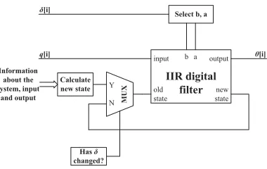
[image:5.594.63.287.327.541.2]The difficulty posed by this approach is that there is no di-rect conversion between the internal state vectors of two differ-ent filters. A technique must, therefore, be developed to allow bumpless (i.e., smooth) transition between filters such that the modeled state of the system remains consistent as filter param-etersbandaare substituted. Fig. 7 shows the procedure used.
Fig. 7. Digital filter arrangement showing the need to recalculate the filter state vector after a change in active cooling.
When there is no change in blower speed, the temperature esti-mation is simply the output of the digital filter to the power input (with the state vector zeroed initially); however, when there is a change in blower speed, a new digital filter is selected and a new state is calculated based on information about the system.
When the blower speed changes, the filter in use is changed to the appropriate filter for the new blower speed. However, the internal filter states, which is the filter’s memory of its previous input, must be determined for the new filter such that the internal state reflects the current system state. It is not possible to directly convert the state of the previous filter to that for the new filter because the vectorsbandamay be significantly different, even for similar cross coupling characteristics.
Techniques commonly used in control engineering for similar purposes are bumpless transfer from manual to automatic con-trol [18] and gain scheduling for nonlinear concon-trollers whose op-erating domain has been divided into several approximately lin-ear subdomains [19]. These methods are applicable where one or more closed-loop controllers are in operation. The proposed esti-mator is an open-loop system, however, and therefore advanced control techniques such as these are not required. Bumpless transition at filter substitution is instead achieved using simple scaling. It is shown below that this approach produces results with minimal error compared to experimental verification.
A. Proposed Methods for Bumpless Digital Filter Transition
Two easy-to-implement methods are available to determine the new state. In the first, the new filter can be set to its steady-state value. This steady-state may be found mathematically and is scaled such that that the output temperature remains correct (i.e., without a bump) when the new filter is substituted. This ap-proach has the disadvantage that the history of the input power to the system, stored in the filter state, is lost. Alternatively, to counteract this problem, the filter state can be determined by providing the filter with the same input waveform that the pre-vious filter received. The input and output values to the filter can then be scaled to ensure the correct output is produced at the point of substitution to ensure bumplessness. Because the new filter has processed the entire input waveform, its state vec-tor more accurately represents the true state of the system. The properties of these two techniques are described later.
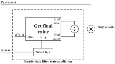
Fig. 8. Filter state recalculation technique for the steady-state assumption method. This replaces calculate new state in Fig. 7.
vectorsto the appropriate steady-state level for the last output of the previous filter. This vector is found using the z-domain final value theorem [20], which states that the final value of the sequence can be calculated as
θ[∞] = lim
t→∞θ(t) = limz→1(z−1) Θ (z)
= lim
z→1(z−1)Zth(z)Q(z). (12)
To calculate the final value steady state in steady state,q(t)
is 1 W for allt, therefore [17]
Q(z) = z
z−1. (13)
Having determinedθ[∞], the values of the of the state vector can be calculated by solving (11) for a constant state vector and the final temperature, as shown in
sL−1=bL+ 0−θ[∞]aL
sL−2=bL−1+sL−1−θ[∞]aL−1
.. .
s0 =b1+s1−θ[∞]a1.
(14)
The technique is shown in Fig. 8. The state vector is normal-ized by dividing the state by the final temperature,θ. Upon filter change, the normalized state vector of the new filter is scaled to the correct value by multiplying by the final output temperature of the previous filter. Scaling in this way is valid because digital filters are linear [17].
This steady-state method assumes that when the blower speed is changed, the system is in steady state. Because the memory of previous input is lost, this assumption is limited to cases where the filter has stabilized or where there is no significant delay between power input and response. The method is useful, however, because the steady-state vector s can be calculated efficiently.
To illustrate the operation of the technique in practice, device 1 shown in Fig. 2 was set to dissipate selected power waveforms and levels of active cooling while the temperatures of all devices were monitored. The temperature at each device was also esti-mated using the filter technique described above for a blower with speeds of between 0 and 6600 rpm.
Two types of input were selected to illustrate the abilities and limitations of the technique, as described later.
1) A power waveform consisting of three repeats of the Eu-ropean driving cycle waveform [21] was chosen due its
wide range of powers and changes of rates (for the sake of simplicity, power is taken as proportional to the velocity parameter in the cycle). A blower waveform consisting mainly of gradual changes was applied during the cycles, meaning a new state must regularly be calculated for the filter. These inputs represent a difficult real-world problem for the estimator.
2) A set of inputs consisting of irregular and rapid arbitrary changes in power and blower speeds was chosen. For these inputs, only occasional state recalculations are required and the consequent error in calculating the filter state is smaller.
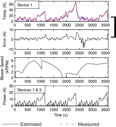
For both waveforms, the power input was applied to device 1 with the temperature responses measured at devices 1 and 3 (i.e., the auto and cross-coupling responses, respectively) measured. The results are shown in Fig. 9.
For the gradual changes in Fig. 9(a), the agreement with practical results is excellent for device 1 (the auto coupling case) with the root-mean-square error (RMSE) between the estimation and practical results being 1.9 K. In the case of the device 3 (cross coupling), however, there is a significant difference between estimated and practical results demonstrated by an RMSE of 4.9 K. This inaccuracy is caused by the loss of memory due to the steady-state assumption method removing the effect of past frequency input from the filter’s internal state. In the case of auto coupling, the time constants of the thermal response are short and, therefore, the effect of inputs some time ago is limited. However, when cross coupling is considered, the time constants are longer and the full effect of a change in input power is not given time to appear before there is another filter change. For frequently changing input, erasing the memory by repeatedly reinitializing the filter to steady state invalidates the estimations. The issues are highlighted where only irregular sudden changes in blower speed occur, such as in Fig. 9(b). In this case, the error is similar in both the auto and cross coupling cases (with RMSEs of 2.1 and 1.3 K, respectively) because there is no significant memory loss. For this reason, a technique that does not erase memory of previous inputs is required for accurate temperature estimations under constantly changing cooling in the case of cross coupling.
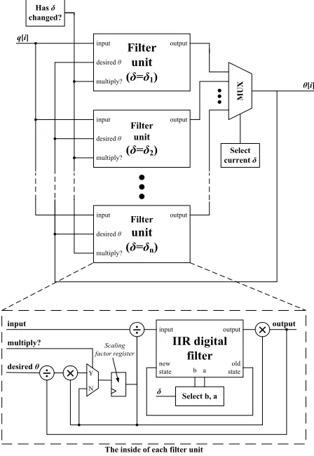
2) Scaled Input Assumption Method: An alternative approach is to assume that the new filter has experienced the same input as the old filter. The frequency content of the new filter’s state vector will, therefore, be the same as the previous filter, al-though the old and new filter states may have little numerical resemblance. To achieve this effect, state vectors for all fil-ters are maintained irrespective of whether they are presently required. These vectors are updated at each time step, and a nor-malization procedure is implemented, where there is a change of blower speed. The full procedure for the scaled input assumption method is shown in Fig. 10.
The full range of blower speeds is quantized into discrete levelsδ1toδnto limit the number of filters (and therefore
Fig. 9. Estimated and actual temperature responses at device 1 (auto coupling) and device 3 (cross coupling) due to power dissipation in device 1 under variable blower speed for the steady-state assumption method. Large square brackets between graphs link a device temperature result with its error. Results for system under (a) gradual frequent changes of blower speed, and (b) pronounced infrequent blower speed changes.
is selected as the active temperature estimation output. Ifδdoes not change, the method is identical to the single filter method described in Section III-B, except that other filters are silently calculating their response and updating their state vectors.
When a change of blower speed occurs (and thus the multiply? flag in Fig. 10 is set), all the filters have their output normalized to the estimated temperature immediately preceding the change. To achieve this, a scaling factor is calculated to produce the cor-rect output temperature immediately following the change of filter. The input power must also be scaled by the reciprocal of the output scaling factor to maintain correct frequency response of the filter unit. The scaled assumption method is more com-putationally intensive than the steady-state assumption method because it requires several filters to be simultaneously main-tained. However, owing to the long time constants involved in thermal systems, a new temperature value is only occasionally input (every 4.6 s in our example). This allows sufficient time to recalculate each filter using a typical microcontroller. The computational requirements are described in Section V.
For verification, the scaled input assumption method was applied to the same arbitrary power and blower waveforms as in the previous section. The model was quantized to one filter for each multiple of 50 rpm to reduce memory and processing requirements. Results are shown in Fig. 11. For the auto coupling response of device 1, the method shows little improvement over the steady-state method, with similar RMSEs of 1.2 and 1.4 K for Fig. 11(a) and (b), respectively. For cross coupling, however, there is a significant improvement in the closeness of the estimation for the regularly changing
Filter unit ( = 1)
desired
output input
multiply?
MUX
Filter unit
( = 2)
desired
output input
multiply?
Filter
unit ( = n)
desired
output input
multiply?
Select current
q[i] Has changed?
IIR digital filter
new state
output
old state
Select b, a
input
b a
input
multiply?
desired
output [i]
The inside of each filter unit
Y
N
Scaling factor register
[image:7.594.313.537.398.723.2]Fig. 11. Estimated and actual temperature responses at device 1 (auto coupling) and device 3 (cross coupling) due to power dissipation in device 1 under variable blower speed for the scaled input method. (a) Under gradual frequent changes of blower speed. (b) Under pronounced infrequent blower speed changes.
blower speed seen in Fig. 11(a). The error is similar to that of the auto coupling response at 1.4 K, a 70% reduction over the steady-state technique. In addition, the shapes of the curves are similar. The irregular power and blower speed test in Fig. 11(b) shows similar results to the steady-state assumption technique (RMSE of 1.1 K), confirming that regular changes in blower speed increase the need for complex filter conversion.
B. Temperature Response With Multiple Devices Dissipating
Results presented so far are for a single device dissipating power. However, the techniques presented in this paper are equally applicable in cases where multiple devices are dissipat-ing. Fig. 12 shows estimated and actual temperature at device 1, where both devices 1 and 3 are dissipating the European driving cycle-based power waveform under slow-changing cooling. The estimated response is calculated using (2) by adding the individ-ual estimated temperature response at device 1 due to dissipation at device 1 alone to the response due to device 3 alone. For this estimation, the scaled input assumption method was used.
The agreement between estimated and practical results is excellent and is comparable to the results for a single vice, demonstrating the technique’s viability for multiple de-vice temperature estimation. Errors compared to practical re-sults are small with occasional increases during periods of rapid temperature change. The profile of the temperature estimated and practical responses are the same with correctly estimated peaks and gradients, making the results appropriate for relia-bility modeling and cooling control. This is confirmed by the RMSE of 2.0 K, which represents an insignificant error for most practical purposes.
Fig. 12. Estimated and actual temperature responses at device 1 due to equal simultaneous power dissipation in devices 1 and 3 under variable blower speed.
V. PRACTICALIMPLEMENTATION ON AMICROCONTROLLER
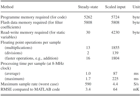
[image:8.594.331.529.373.590.2]TABLE I
COMPUTATIONALREQUIREMENTS PERDEVICEPAIR FOR THE
PROPOSEDMETHODS
Method Steady-state Scaled input Unit
Programme memory required (for code) 5262 5724 byte Flash data memory required (for filter
coefficients)
5808 5808 byte
Read-write memory required (for static variables)
30 4230 byte
Floating point operations per sample
(multiplications) 13 1855
(divisions) 2 139
(faster operations, e.g., addition) 16 1804 Processing time per sample (at 8-MHz
clock)
(average) 1.0 87 ms
(maximum) 1.7 225 ms
Maximum sample rate (worst case) 590 4.4 S/s RMSE compared to MATLAB code 3.4 64 mK Conditions: 4.6-s sampling period; 132 quantized cooling levels for both methods.
instead implemented in software). This low cost and moderate performance microcontroller was selected to illustrate the low-computational requirements of the proposed technique. Indeed, although capable of 20 MHz, the microcontroller was clocked using the internal 8-MHz RC timer to further demonstrate that the proposed technique can be implemented on basic hardware. Where the requirements of a particular application require a higher iteration rate, higher specification microcontrollers are economically available.
The C++ code was a functionally identical rewrite of the MATLAB development code, with platform alterations to account for the limitations of a microcontroller. In particular, the polynomial coefficient vectorsbandaare stored in the flash memory (which can be written to by the software) and all data is stored as single-precision (32-bit) floating point numbers. For test purposes, the response to the European driving cycle power with gradually but infrequently changing blower speed inputs, as used in Fig. 9(a) in Fig. 11(a), was calculated using the microcontroller. Near identical results were obtained (with a RMSE between MATLAB-based results and microcontroller generated results of less than 63 mK, as a result of floating point precision differences).
Table I shows the computational resources required to imple-ment the program and calculate the temperature response on the microcontroller. Flash data memory, where the filter vectorsb
[image:9.594.44.282.100.263.2]andaare stored, is identical for both methods because the same filters are used. The scaled input assumption method requires significantly more read–write memory and floating point opera-tions per sample to maintain the additional state vectors needed by that method. The difference between the program memory requirements is insignificant because the code base is very sim-ilar. The scaled input assumption method is significantly slower (allowing only 4.4 samples/s for the worst case, compared to 590); however, this is more than sufficient for typical systems such as the demonstrator system. To achieve greater speeds, a dedicated digital signals processing controller could instead be used. Because the computational requirements of both methods are fulfilled by typical microcontrollers, the scaled input assumption method is preferred since it produces better results.
Fig. 13. Design stage procedure to generate models and characteristics.
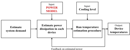
VI. PROCEDURE FORAPPLICATION TO APOWERCONVERTER
The techniques discussed in the paper are applicable to a wide range of thermal systems under variable active cooling. The pro-cedure for implementing the technique can be divided into two parts: (A) design stage modeling and characterization and (B) implementation in the operational system. The considerations for these stages are described later.
A. Design Stage Modeling and Characterization
Fig. 13 presents a suggested procedure for implementing the technique for a typical power converter. Initially, the power con-verter is designed and laid out according to normal engineering principles. Because the proposed temperature estimation tech-nique requires real-time power dissipation data as an input, an electrical power model of the circuit is required. This model can be developed in a number of ways and the literature has extensive examples of viable approaches. For example, Capua and Femia [22] produce a computationally efficient model for a MOSFET switching circuit by first principles analysis of the structure of a MOSFET. Orabi and Shawky [23] take this ap-proach further by calculating the power losses of a MOSFET with respect to load, a procedure that could be applied to the present study to calculate losses in the active devices with re-spect to demand on the circuit. Whatever approach is taken, a circuit-specific model is generated, which relates demand on the power converter prototype to power losses in each device.
Fig. 14. Program flowchart for each iteration of temperature estimation on the operational system.
with test points on the prototype PCB using a modified bed-of-nails tester.
Following the procedure outlined in Section II-B, the thermal cross coupling of the system is characterized over an appropri-ate range of cooling levels. Because an active device is being used instead of the illustrative resistor used in Section II-B, an additional circuit, such as the one reported in [24], is required to control the power in each device. This circuit is required only for characterization and will, therefore, be external to the proto-type. The temperature response of each device may be measured using a nonintrusive method such as with a single pixel thermal camera. Using the procedure described in Section II, the thermal characteristics are produced and this forms the thermal model of the system.
B. Implementation Within the Operational System
Having generated the models on a prototype system, the tem-perature estimation technique can be realized on the operational system. The flowchart of the required program is shown in Fig. 14. At each time step, the demand on the system is es-timated. Depending on the application, this might be through measurement of the output current (e.g., on a simple power con-verter) or through measurement of the work done (e.g., water throughput when designing a drive for a pump). Using the power model developed as part of the design stage modeling, estimates of the power in each device are produced. Since losses in de-vices may be temperature dependent, the estimated temperature is used as an additional input to the model. The temperature estimation procedure described in Section IV and implemented in Section V is then employed to produce real-time temperature data, which is, hence, available for such purposes as cooling control, demand management or for any other purpose.
VII. DISCUSSION
A. Implementation Decisions
This paper has proposed a method of estimating the tem-perature of devices under variable cooling. The technique is applicable in several areas, notably for air- and liquid-cooled power electronics in drive systems. To implement the estimator in practice, two decisions must be made. First, which of the proposed methods will be used for the transition between filters must be chosen. It was shown in Section IV that for cases where the response is mainly due to auto coupling or where changes in cooling level are infrequent, the simpler steady-state assumption
method may suffice. However, where there is a delay between input and output (in the case of cross coupling, for example) and frequent changes in cooling level, a more involved method is required. The engineer must decide whether the additional computational requirements are justified by the increased accu-racy. That is a complex application-specific question involving the budget for the particular system versus the desire for tight thermal control. We have seen that both methods can be imple-mented on a cheap 8-bit microprocessor running on a low-speed RC clock. There is, therefore, a strong preference for the scaled input method except in the case high sample rate systems con-sisting of many devices. Alternatively, thermal management of complex systems could be implementation on a digital signals processor to allow increased processing rates through acceler-ated mathematics.
The second decision is the level of quantization desired between cooling levels. An increased number of steps offers greater model acuity at the expense of processor requirements (memory and sample rate), which scale linearly with number of discrete cooling levels. Additionally, for very finely quan-tized models, transitions between filters become undesirably frequent. In this case, transitions may occur where there is no significant difference in actual cooling or merely as a result of noise in cooling level measurement. The degree of quantization is, therefore, also application specific.
B. Comparison to Related Work
Techniques for device temperature estimation and prediction on a system under variable cooling have received relatively little attention in the recent literature, with many authors preferring to use a thermal model that assumes consistent cooling [8], [9]. These methods lose accuracy under variable cooling. Al-ternatively, authors use methods that measure the temperatures under variable cooling directly, without an estimator (one such example is [25]). These methods, on the other hand, increase the per-unit system cost through the increased requirement for sensors and signal conditioning. Finally, alternative proposals that do produce temperature estimations under variable cooling often calculate the change in the parameters of thermal equiva-lent circuits and produce a SPICE model [26]. Although these estimation techniques generate results of similar accuracy to the technique proposed in this paper, the requirement to produce an accurate equivalent circuit model and identify which parameters are affected by cooling increases the design effort required for implementation.
VIII. CONCLUSION
systems with infrequent changes in power dissipation or cooling level. However, greater accuracy is achieved using the second technique, which duplicates the frequency content of the existing filter’s state by exposing it to the same input. The estimation techniques demonstrate accurate tracking of temperature with minimal error when compared with the experimental data.
REFERENCES
[1] M. Gerber, J. A. Ferreira, N. Seliger, and I. W. Hofsajer, “Integral 3-D thermal, electrical and mechanical design of an automotive 3-DC/3-DC converter,” IEEE Trans. Power Electron., vol. 20, no. 3, pp. 566–575, May 2005.
[2] V. Smet, F. Forest, J.-J. Huselstein, F. Richardeau, Z. Khatir, S. Lefebvre, and M. Berkani, “Ageing and failure modes of IGBT modules in high-temperature power cycling,” IEEE Trans. Ind. Electron., vol. 58, no. 10, pp. 4931–4941, Oct. 2011.
[3] H. Lu, C. Bailey, and C. Yin, “Design for reliability of power electronics modules,” Microelectron. Rel., vol. 49, no. 9–11, pp. 1250–1255, Sep.– Nov. 2009.
[4] P. Ning, G. Lei, F. Wang, and K. D. T. Ngo, “Selection of heatsink and fan for high-temperature power modules under weight constraint,” in Proc.
23rd Annu. IEEE Conf. Appl. Power Electron. Conf. Expo., Feb. 2008,
pp. 192–198.
[5] L. Meysenc, M. Jylhakallio, and P. Barbosa, “Power electronics cool-ing effectiveness versus thermal inertia,” IEEE Trans. Power Electron., vol. 20, no. 3, pp. 687,693, May 2005.
[6] L. Fried, “Prediction of temperatures in forced-convection cooled elec-tronic equipment,” IRE Trans. Compon. Parts, vol. CR-5, no. 2, pp. 102–107, Jun. 1958.
[7] C. Lundquist and V. P. Carey, “Microprocessor-based adaptive thermal control for an air-cooled computer CPU module,” in Proc. 17th Annu.
IEEE Symp. Semicond. Therm. Meas. Manag., 2001, pp. 168–173.
[8] M. Musallam and C. M. Johnson, “Real-time compact thermal models for health management of power electronics,” IEEE Trans. Power Electron., vol. 25, no. 6, pp. 1416–1425, Jun. 2010.
[9] G. C. James, V. Pickert, and M. Cade, “A thermal model for a multichip device with changing cooling conditions,” in Proc. 4th IET Conf. Power
Electron., Mach. Drives, 2008, pp. 310–314.
[10] G. Xiong, M. Lu, C.-L. Chen, B. P. Wang, and D. Kehl, “Numer-ical optimization of a power electronics cooling assembly,” in Proc.
IEEE 16th Annu. Appl. Power Electron. Conf. Expo., 2001, vol. 2,
pp. 1068–1073.
[11] P. J. Rodgers, V. R. C. Eveloy, and M. R. D. Davies, “An experimental assessment of numerical predictive accuracy for electronic component heat transfer in forced convection—part I: Experimental methods and numerical modeling,” J. Electron. Packag., vol. 125, pp. 67–75, 2003. [12] P. J. Rodgers, V. R. C. Eveloy, and M. R. Davies, “An experimental
assessment of numerical predictive accuracy for electronic component heat transfer in forced convection—part II: Results and discussion,” J.
Electron. Packag., vol. 125, pp. 76–83, 2003.
[13] J. N. Davidson, D. A. Stone, and M. P. Foster, “Real-time prediction of power electronic device temperatures using PRBS-generated frequency-domain thermal cross-coupling characteristics,” IEEE Trans. Power
Elec-tron., vol. 30, no. 6, pp. 2950–2961, Jun. 2015.
[14] J. N. Davidson, D. A. Stone, M. P. Foster, and D. T. Gladwin, “Im-proved bandwidth and noise resilience in thermal impedance spectroscopy by mixing PRBS signals,” IEEE Trans. Power Electron., vol. 29, no. 9, pp. 4817–4828, Sep. 2014.
[15] B. Miao, R. Zane, and D. Maksimovic, “System identification of power converters with digital control through cross-correlation methods,” IEEE
Trans. Power Electron., vol. 20, no. 5, pp. 1093–1099, Sep. 2005.
[16] MathWorks. (2013, Jul. 8).. MATLAB 2013a documentation: In-vfreqz[Online]. Available: http://www.mathworks.co.uk/help/signal/ref/ invfreqz.html.
[17] A. V. Oppenheim and R. W. Schafer, Discrete-Time Signal Processing. Englewood Cliffs, NJ, USA: Prentice-Hall, 1999.
[18] R. Hanus, M. Kinnaert, and J.-L. Henrotte, “Conditioning technique, a general anti-windup and bumpless transfer method,” Automatica, vol. 23, no. 6, pp. 729–739, Nov. 1987.
[19] J. D. Bendtsen, J. Stoustrup, and K. Trangbaek, “Bumpless transfer be-tween observer-based gain scheduled controller,” Int. J. Control, vol. 78, no. 7, pp. 491–504, 2005.
[20] E. W. Kamen, Introduction to Signals and Systems. New York, NY, USA: Macmillan, 1990, pp. 333–334
[21] European Community, “Directive 90/C81/01,” EEC Journal Officiel No. C81, 30 Mar. 1990, p. 110.
[22] G. Di Capua and N. Femia, “A versatile method for MOSFET commu-tation analysis in switching power converter design,” IEEE Trans. Power
Electron., vol. 29, no. 3, pp. 920–935, Feb. 2014.
[23] M. Orabi and A. Shawky, “Proposed switching losses model for integrated point-of-load synchronous buck converters,” IEEE Trans. Power Electron., vol. 30, no. 9, pp. 5136–5150, Sep. 2015.
[24] J. N. Davidson, D. A. Stone, and M. P. Foster, “Arbitrary waveform power controller for thermal measurements in semiconductor devices,” Electron.
Lett., vol. 48, no. 7, pp. 400–402, 2012.
[25] C. E. Bash, C. D. Patel, and R. K. Sharma, “Dynamic thermal manage-ment of air cooled data centers,” in Proc. 10th Intersoc. Conf. Therm.
Thermomech. Phenom. Electron. Syst., 2006, pp. 8–452.
[26] M. M¨arz and P. Nance, Thermal Modeling of Power Electronic Systems Munich, Germany: Infineon Technologies AG, 2000.
Jonathan N. Davidson received the M.Eng. degree
in electronic engineering and the Ph.D. degree in ther-mal modeling and management from the University of Sheffield, Sheffield, U.K., in 2010 and 2015, re-spectively.
He is currently a Research Associate at the Univer-sity of Sheffield. His research interests include ther-mal modeling and management of power electronics, and design of piezoelectric power converters.
Dr. Davidson is a Member of the Institution of Engineering and Technology.
David A. Stone received the B.Eng. degree in
elec-tronic engineering from the University of Sheffield, Sheffield, U.K., in 1984 and the Ph.D. degree from Liverpool University, Liverpool, U.K., in 1989.
He then returned to the University of Sheffield as a Member of academic staff specializing in power electronics and machine drive systems. His current research interests include hybrid-electric vehicles, battery management, electromagnetic compatibility, and novel lamp ballasts for low-pressure fluorescent lamps.
Martin P. Foster received the B.Eng. degree in
elec-tronic and electrical engineering, the M.Sc. (Eng.) de-gree in control systems, and the Ph.D. dede-gree for his thesis “Analysis and Design of High-order Resonant Power Converters” from the University of Sheffield, Sheffield, U.K., in 1998, 2000, and 2003, respec-tively.
In 2003, he became a Member of academic staff at Sheffield specializing in power electronic systems and was made a Senior Lecturer in 2010 and then a Reader in 2014. His current research interests include the modeling and control of switching power converters, resonant power sup-plies, multilevel converters, battery management, piezoelectric transformers, power electronic packaging, and autonomous aerospace vehicles.
Daniel T. Gladwin received the M.Eng. (Hons.)
de-gree in electronic engineering (computer architec-ture) and the Ph.D. degree in automated control struc-ture design and optimization using evolutionary com-puting from the University of Sheffield, Sheffield, U.K., in 2004 and 2009 respectively.