Cross-Modality Image Synthesis via Weakly-Coupled and Geometry Co-Regularized Joint Dictionary Learning

Geometry Co-Regularized Joint Dictionary Learning

.

White Rose Research Online URL for this paper:

http://eprints.whiterose.ac.uk/128920/

Version: Accepted Version

Article:

Huang, Y., Shao, L. and Frangi, A.F. orcid.org/0000-0002-2675-528X (2017)

Cross-Modality Image Synthesis via Weakly-Coupled and Geometry Co-Regularized Joint

Dictionary Learning. IEEE Transactions on Medical Imaging, 37 (3). pp. 815-827. ISSN

0278-0062

https://doi.org/10.1109/TMI.2017.2781192

[email protected] https://eprints.whiterose.ac.uk/

Reuse

Items deposited in White Rose Research Online are protected by copyright, with all rights reserved unless indicated otherwise. They may be downloaded and/or printed for private study, or other acts as permitted by national copyright laws. The publisher or other rights holders may allow further reproduction and re-use of the full text version. This is indicated by the licence information on the White Rose Research Online record for the item.

Takedown

If you consider content in White Rose Research Online to be in breach of UK law, please notify us by

Cross-Modality Image Synthesis via

Weakly-Coupled and Geometry Co-Regularized

Joint Dictionary Learning

Yawen Huang,

Student Member, IEEE,

Ling Shao,

Senior Member, IEEE,

and Alejandro F. Frangi,

Fellow, IEEE

Abstract_{—Multi-modality medical imaging is increasingly used} for comprehensive assessment of complex diseases in either diagnostic examinations or as part of medical research trials. Different imaging modalities provide complementary information about living tissues. However, multi-modal examinations are not always possible due to adversary factors such as patient discomfort, increased cost, prolonged scanning time and scanner unavailability. In addition, in large imaging studies incomplete records are not uncommon owing to image artifacts, data corruption or data loss, which compromise the potential of multi-modal acquisitions. In this paper, we propose a Weakly-coupled And Geometry co-regularized (WAG) joint dictionary learning method to address the problem of cross-modality synthesis while considering the fact that collecting large amounts of training data is often impractical. Our learning stage requires only a few registered multi-modality image pairs as training data. To employ both paired images and a large set of unpaired data, a cross-modality image matching criterion is proposed. We then propose a unified model by integrating such a criterion into the joint dictionary learning and the observed common feature space for associating cross-modality data for the purpose of synthesis. Furthermore, two regularization terms are added to construct robust sparse representations. Our experimental results demonstrate superior performance of the proposed model over state-of-the-art methods.

Index Terms—Dictionary Learning, Sparse Representation, Image Synthesis, Domain Adaption, Manifold Learning, MRI.

I. INTRODUCTION

M

AGNETIC Resonance Imaging (MRI) is a versatile and noninvasive imaging technique extensively used in neuroimaging studies. MRI comes in several modalities, for example, Proton Density (PD)-weighted images distinguish between fluid and fat, whereas T1weighted scans have good tissue contrast between gray matter and white matter. Each modality offers diverse and complementary image contrast mechanisms unraveling structural and functional information about brain tissue. Due to variations in the brain images across modalities, multi-modality MRI is preferred in many pharma-ceutical clinical trials, in research studies of neurosciences, or in population imaging cohorts targeting to understand neurode-generation and cognitive decline. However, the acquisitions

Y. Huang and A.F. Frangi are with the Center for Computational Imaging and Simulation Technologies in Biomedicine (CISTIB), De-partment of Electronic and Electrical Engineering, The University of Sheffield, Sheffield, United Kingdom (e-mail: [email protected], [email protected]).

L. Shao is with the School of Computing Sciences, University of East Anglia, Norwich, United Kingdom (e-mail: [email protected]).

of a full battery of all these MR images can face constraints associated with their cost, limited availability of scanning time, patient comfort or safety considerations. In large scale studies, it is not uncommon to face incomplete datasets since the presence of imaging artifacts, acquisition errors or corrupted data. While various post-processing solutions such as image imputation [1] and histogram matching [2, 3] have been proposed to compensate for these latter issues, this is usually only at the level of derived imaging biomarkers but not of the data itself [4, 5]. Finally, in longitudinal imaging studies where images are collected over several years, evolution of imaging technology may lead to the appearance of new MRI sequences added to an existing imaging protocol in time, which were not available as part of the imaging battery acquired at earlier time points. In these and other applications, it would be desirable to have a cross-modality image synthesis method that can generate the target modality images from the source modality scans. The ability to synthesize different modalities of the same anatomy can benefit various practical image analysis tasks including multi-modal registration [6, 7], segmentation [8], and atlas construction [9, 10].

In the last few years, cross-modality image synthesis has attracted the attention of the medical image computing com-munity. Most techniques assume such mapping exists between source and target imaging modalities. The problem is then formulated as that of learning the most efficient mapping representation. To synthesize the target from a source modality, some methods have been proposed that construct a dictionary from patches extracted from a single image or from image pairs [4, 11–13] or that learn the mapping from a large set of training image pairs [14–17]. Although these approaches have shown great promise, they are supervised and require labeled data sets.

In this paper, instead, we propose a single-image cross-modality synthesis method with an application to T1w, T2w and PDw brain MRI that utilizes a few registered multi-modality image pairs1_{while employing a larger set of unpaired} data for synthesizing the target image modality from an avail-able source image modality. Our method extracts the common latent features that map different image features of the underly-ing tissues, preserves global statistical image properties across modalities, and simultaneously, refines extracted features to preserve the local geometrical structure in each modality. In

addition, the proposed approach requires only a few registered image pairs to find the mapping between the appearances in different image modalities and employs auxiliary unpaired training images to further exploit the modality-specific ge-ometric structure and obtain a robust sparse representation. To complement the unpaired data with the original training pairs, manifold ranking-based cross-modality image matching is employed as a criterion to pick up features of the target domain from most similar subjects in the source domain. The mapping between multi-modality data can be complex and highly nonlinear. To provide the needed flexibility to map image structures in different modalities, we determine a common feature space by an association function that describes and relates cross-modality data. We call the proposed method Weakly-coupled And Geometry (WAG) co-regularized joint dictionary learning, and perform extensive experiments to verify its performance.

The contributions of this work are threefold:

(1) WAG is a unified model, which learns a pair of (not coupled) dictionaries with a common feature space for medical imaging cross-modality synthesis. WAG automat-ically trains dictionary pairs and computes an association function between source and target modality data based on only a few registered image pairs;

(2) To enrich this model, we design a cross-modality image matching criterion that acts collaboratively with a larger set of unpaired images. This allows identifying correspon-dences across source and target domains that are invariant to pose transformations;

(3) We deal with the considerable difference in data dis-tributions from different modalities (i.e. T1w, T2w and PDw MRI) by simultaneously minimizing the distribution discrepancy of similar instances and preserving geometric structures in each domain.

A preliminary version [5] of this work was presented earlier at the SASHIMI Workshop in MICCAI 2016 (www.cistib.org/sashimi2016). This work adds to the seminal version in significant ways. First, we improve the synthesis model by introducing a cross-modality image-matching crite-rion to connect and integrate all information from both regis-tered and unregisregis-tered data in different modalities to describe the diversity of human brain imaging. Second, we extend the single geometry regularization by preserving modality-specific local geometric properties to penalize undesired loss of information. Third, we consider the flexibility of domain-specific information and construct a common feature space by a mapping function that describes and associates cross-modality data. Fourth, we also extend the original experiments from only comparing with one baseline method to several recently published approaches involving both supervised and unsupervised settings. The proposed method demonstrates state-of-the-art synthesis results using two evaluation metrics in all of our experiments.

The remainder of this paper is organized as follows. Section II reviews related work. Section III defines the cross-modality synthesis problem and introduces our proposed method. The experimental results are demonstrated in Section IV with

discussions. The discussion of this work is given in Section V. Section VI concludes the paper.

II. RELATEDWORK

To synthesize a target modality image from a source modal-ity image, several approaches have been suggested in the literature with promising results [13, 15, 16]. Most of these methods can be broadly referred to asexample-based methods

and roughly subdivided based on the size of the training set. Example-based methods learn the source-target mapping from a very small number of source-target image pairs (e.g.

several or even a pair of images) by extracting multiple image patches from the source image and assuming the same sparse codes are shared between source and target modality spaces. One of the well-established cross-modality synthesis approaches in this category is Hertzmann et al.’s image analogies [11], which transfers the texture information from a source modality space onto a target modality space. The same strategy is also applied to facilitate multi-modal image registration in correlative microscopy [6]. Kroon et al. [18] mapped between T1w and T2w magnetic resonance images by simply using the peaks in a joint histogram of registered image pairs to transform between source and target image representations. Techniques based on sparse representations have been presented, which separately learn two corresponding dictionaries from registered image pairs and synthesize the target MRI modality data from the patches of the source MRI modality [4]. Recently, Jog et al. [13] proposed a nonlinear regression-based image synthesis approach that used registered image pairs to train a random forest regressor for predicting the target from the source image intensity.

Projected Common Feature Space

RKHS For

For MMD term Graph Co-regularization term Dictionary Pairs

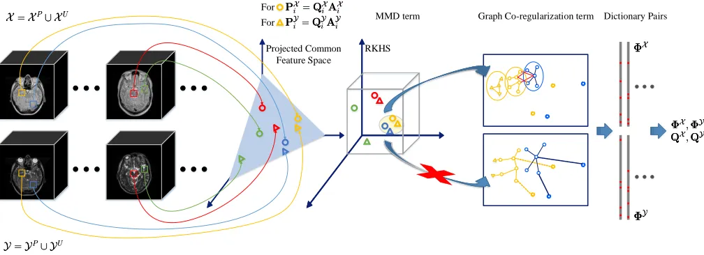
Fig. 1. Overview of the proposed cross-modality image synthesis method. Squares within the 3D images represent the extracted 3D patches with size of 5×₅×_{5. The first step is to project the extracted paired/unpaired patches into a common feature space denoted by circles for source modality data and triangles}

for target modality data respectively. Then, we measure the divergence of the distribution of the maximum mean discrepancy (MMD) over all matched pairs from the first step to seek the intrinsic pairs in the reproducing kernel Hilbert space (RKHS). After that, to better preserve the modality-specific information, we adopt the Laplacian eigenmaps to capture the local geometric structure for each domain and denoted by geometric co-regularization term. Finally, the expected dictionary pairs can be trained based on the processed features.

for synthesis. Instead of using coupled image pairs as training data, matching feature representations and learning spatial relations with joint sparse coding [15] has shown great poten-tial in synthesizing images across modalities. To improve the quality of the synthesized images across different modalities, Huang et al. [20] proposed to first align weakly-supervised data and then generate super-resolution cross-modality data si-multaneously using joint convolutional sparse coding scheme. Inspired by this strategy, we integrate paired and unpaired training data by constructing correspondences across different modalities and leverage weakly-coupled data effectively.

As argued in [15], collecting a large number of multi-modality images is both time-consuming and expensive, and sometimes even impractical in medical imaging. Most of the methods, especially the full-set-based approaches, require con-siderable amounts of co-registered training data in both source and target domains. Motivated by this and the above works, we propose a more practical cross-modality image synthesis solution that links source-target domains in a weakly-coupled fashion, which outperforms existing state-of-the-art methods on several experimental scenarios.

III. METHOD

In this section, we first formulate the problem formally. Then, we propose a general framework for cross-modality image synthesis. Our approach extends the conventional dictio-nary learning approach by jointly learning a pair of dictionaries from the constructed common feature space that describes and associates cross-modality data. We also consider the minimiza-tion of the distribuminimiza-tion divergence between both modalities while preserving modality-specific local geometric properties that penalize undesired loss of information. Finally, we utilize unpaired images in both domains as auxiliary training data that enhances the supervised learning process. This additional unsupervised step collaborates with and complements the

registered training image pairs. An overview of our proposed method is depicted in Fig. 1.

A. Problem Definition

LetX ={X1, ...,XS}be the source modality images ofS

subjects using modality M1, and Y ={Y1, ...,YT} be the

target modality images of T subjects imaged using modality

M2. Therefore,Xi andYi represent the i-thsubject-specific

images for each modality, and S and T indicate the total numbers of samples in each corresponding training set. Each domain is broken down into a registered/paired domain subset of size R, i.e., XP _{= {X}

1, ...,XR}, YP = {Y1, ...,YR},

and an unregistered/unpaired domain subset of size T −R or S − R, respectively, i.e. _XU _{= {X}

R+1, ...,XS},

YU _={Y

R+1, ...,YT}soX =XP∪XU andY=YP∪YU.

The assumption here is that R ≪ S, T and we only need access to a few registered pairs and a much larger set of unpaired images. Images in the setsX andY are represented asm×nmatrices whose columns are each of the 3D patches vectorized in lexicographic order. Hence, image data matrices

X = [x1, ...,xn] ∈ Rm×n and Y = [y1, ...,yn] ∈ Rm×n,

containnoverlapping 3D patches (covering the whole image volume) of dimension m (viz. the cardinality of the 3D patches). The training matrices X and Y are comprised of paired training sub-matrices XP_{, Y}P _{and unpaired training}

sub-matricesXU_,YU_{. We denote the test image in the same}

way by a matrixXt_{. The test 3D patches inX}t _{are acquired}

with modality M1, and will be the input to synthesize the corresponding 3D patches in modalityM2.

Problem Statement: We first denote the coding coefficients

AX,AY of X,Y over the learned dictionariesΦX,ΦY, the projected dataPX,PY ofX,Yin a defined common space, and a mapping function F(·) to represent the relationship between the sparse codes AX

, AY

[image:4.612.56.560.58.241.2]

the detailed descriptions and the corresponding mathematical formulations are provided in the following subsections. Given a pair of training matricesXandY withX=

XP_XU

and

Y=

YP_YU

, our goal is: 1) to learn a pair of dictionaries

ΦX_,ΦY _{, their sparse codes}

AX_,AY _{, and an association} function F(·) : M1 → M2 using the projected data PX and PY_{; and 2) to minimize the inter-modality divergence} between PX _andPY_{, and 3) to preserve the domain-specific} local geometric structure.

B. Dictionary Learning

Assume thatX= [x1, ...,xn]∈Rm×n is a training dataset,

which can be reconstructed by the linear combination of a set of n coefficients that lie on a k-dimensional sparse space,

AX ₌

αX 1, ...,αXn

∈Rk×n _{is associated to the dictionary} ΦX = hφX1, ...,φ

X

k i

∈ Rm×k. Here, k > m to make the dictionary over-complete [21]. Considering the reconstruction error for each data point, the problem of learning a dictionary

ΦX _{for sparse representation ofXcan be formulated as}

min ΦX_,AX

X−ΦXAX

2

F+λ AX

₀, (1)

where k·kF is the Frobenius norm, k·k0 is the l0-norm that penalizes non-zero elements in A, and λ denotes a regular-ization parameter to trade off sparsity vs. reconstruction error. As shown in [22], the minimization problem in Eq. (1) is, in general, NP-hard under the l0-norm. An alternative solution is to relax the l0-norm with the l1-norm and obtain a near-optimal result [23]. The dictionary learning problem in Eq. (1) can be reformulated as

min ΦX_,AX

X−ΦXAX

2

F+λ AX

₁. (2)

The above objective function is not simultaneously convex over Φ and A. A practical solution is to alternate between optimizing for the dictionary Φ and for the sparse codes A

fixing the other degree of freedom. This makes the problem convex and the solution converges to a local minimum [24]. When the dictionary is fixed, the algorithm is known as Lasso/LARS [25] with an l1 penalty over the coefficients and can be solved by the feature-sign search approach [24]. When sparse codes are fixed, such an optimization problem is reduced to a least squares optimization with quadratic constraints, and can be solved using a Lagrange dual [24].

When dealing with multi-modality data, one can simply construct two independent dictionaries using conventional dic-tionary learning. Specifically, given two training data sets X

andY, following the dictionary learning procedure described in [21, 26] and Eq. (2), we can learn the dictionaries separately to obtain the two dictionaries, ΦX and ΦY, and the two corresponding sparse coefficients, AX _andAY_{, respectively.} The data of each modality can be reconstructed using the respective dictionary and associated sparse coefficients.

C. Cross-Modality Dictionary Learning

Cross-modality image synthesis is based on learning a joint sparse representation [19] with a common set of sparse

codes shared between source and target image modalities,

i.e. AX _{≡ A}Y_{. These sparse codes act on independent} dictionaries for each modality,viz.ΦX _andΦY_{, to reconstruct} the corresponding source and target images. To this effect, both 3D patches in the source and target modalities must be perfectly co-registered. To map the tissue appearance across modalities, the joint dictionary learning strategy groups two independent reconstruction errors (viz. X−ΦXAX

2

F and

Y−ΦYAY

2

F) in a single objective function to be

opti-mized:

min ΦX_,ΦY_,A

X−ΦXA

2

F +

Y−ΦYA

2

F+λkAk1 s.t.φX_i

2 2≤1,

φY_i

2

2≤1∀i= 1, ..., k,

(3)

where A denotes the same coefficients to be enforced of registered data pairs projected in a common feature space. As in the single dictionary learning optimization problem, the joint optimization function in Eq. (3) is convex regarding the learned dictionaries, ΦX andΦY, for fixed sparse codes

A. Therefore, the computation of A and of the dictionary pairs can be alternated. Analyzing (3), we note that this objective function is suitable to collaboratively learn a pair of dictionaries, so the sparse codes in the source modality space

M1can directly reconstruct the target modality imageM2in a transferable feature space.

Although joint dictionary learning achieves very good re-sults, it assumes that source and target images, when rep-resented with jointly learned dictionary pairs, ΦX and ΦY, must share the same sparse codes. In addition, all previous work requires that the training dataset contains registered image pairs, which imposes additional demands. In this paper, we address the above problems by relaxing the need for a common sparse representation and providing more flexibility in reducing the registration requirement to a small training dataset only.

D. Weak Coupling and Geometry Co-regularization

To make the proposed method effective for generalized cross-modality synthesis, we combine the following ideas: (1) we integrate paired and unpaired training data in both modalities into a unified framework; (2) we relax the need for a shared sparse code in source and target domains; (3) we allow for dissimilar data distributions as required when dealing with very different image modalities; and (4) we include a mechanism that preserves the local geometric structure specific to the modalities of the source and target images. In the following, we introduce each component, and then summarize our overall approach.

1) Cross-modality image matching: To relate and integrate the information from the paired and unpaired training data subsets of each modality, we introduce a criterion called cross-modality image matching (CMIM) for incorporating the information from the unpaired training data into dictionary learning and cross-modality image synthesis.

features from source and target images where the resolutions of both modalities are similar. This is based on the assumption that tissues may present different visual appearances one each modality but they share similar high order edge/texture characteristics while modality-specific details affect primarily Low-Frequency (LF) properties [19].

In this paper, we follow [19, 27] and adopt first- and second- order derivatives involving horizontal and vertical gradients as the HF features for each training data by Xh= H_∗X, Yh = H_∗Y. Generally, H _{is a high-pass filter} operator used to extract derivatives, Considering first and second order derivatives,H_{is one of the following operators:}

H1 1,H

2 1,H

1 2,H

2

2, where H1

1 = [−1,0,1], H 2 1 = H

1 1

T

, and

H1

2= [−2,−1,0,1,2],H 2 2=H

1 2

T

. Once the features in both domains are computed, we can use them to optimize CMIM and define a mappingC(·) :X → Y. In particular, CMIM can be thought of as a unilateral matching metric (i.e., the weighted regression) that focuses on a particular goal (e.g. matching across resolutions, modalities, or domains. [28–30]). Given associated HF image feature sets, Xh_andYh_{, corresponding}

to both paired and unpaired training image data sets, XP_,

XU_{, Y}P _{and Y}U_{, CMIM represents an ensemble of paired}

and unpaired cross-modality matching sub-problems. Images in XP _{and Y}P _{are endowed with a natural correspondence,}

XP _{⇋ Y}P_{. In contrast, CMIM finds a mapping for}

multi-modality unpaired image data forXU

andYU

. SinceXP

and

YP

are already registered/paired, we can assume a perfect matching between them. By integrating the unpaired image data, we can establish a final affinity matrixTTT∈Rn×n such that C(X,Y) =

Xh−TTTYh

2 2:

T TT=



 

D(xh

1,yh1) · · · D(xh1,yhn)

..

. . .. ... D(xh_n,yh1) · · · D(x

h n,y

h n)





, (4)

whereD(xh_i,yh_j)is a distance function generally designed to measure the distances between each pair of HF feature vectors inX andY using ang-dimensional Gaussian kernel

D(xh_i,yh_j) = 1

(√2πσ)ge

−kx h i−yh_jk2

2σ2 _, (5)

where σ 6= 0 denotes the kernel bandwidth.TTT establishes a one-to-one correspondence for each source domain 3D patch. We preserve the most relevant features with the largest D values within Y while discarding other 3D patches. In this way, fromTTT we defineTTTˆ as:

ˆ T T

T(i, j) =

1, ifj =ji,

0, otherwise. (6)

where ji = maxj(TTT(i, j)) is the maximum element of the i-th row in TTT. Furthermore, we set the maximum element

ˆ T T

T(i, ji)to be 1 where all other values are set to 0 resulting in

a binary assignment matrixTTT. Givenˆ TTT, each source patch isˆ only mapped to one target patch with the most similar tissue texture. Hence, patches across different domains can be treated as the registered pairs after such a processing, i.e., X ⇋ Y

for each xi paired with yji denoted as Pi = {xi,yji} for i= 1. . . n.

2) Computing the mapping function: Starting off by Eq. (2), by minimizing the reconstruction error, the corresponding sparse codesAX _andAY _{for each modality can be computed,} respectively. To allow these codes to differ for the paired exam-ples and unpaired data matched via CMIM, we assume there exists a mapping function F:M1 → M2 withY=F(X). Accordingly, the sparse codes ofXandYover the dictionaries will be related by such a mapping functionF AX_,AY

. To build a stable mapping between two domains, Wang et al.

[31] assumed that the sparse codes from the source domain had to be identical to those for the target domain via a linear projection W. As suggested in [32], projecting both source and target domain data into a common feature space can better describe and associate cross-modality data. Inspired by this strategy, we first define the cross-modality relationship in the projected data PX_{, P}Y _{of X, Y, and replace F(A}X_,AY₎ by F(PX_,PY_{), and then incorporate the projected features} into CMIM-driven coupled dictionary learning. The objective function of this learning model is:

min ΦX_,ΦY_,AX_,AY

X−ΦXAX

2

F+

Y−ΦYAY 2 F +λ AX ₁+ AY ₁ + X h

−TTTˆYh

2

2+νF

PX_,PY ,

(7)

where PX _{= Q}X_AX

∈ Rk×n and PY _{= Q}Y_AY

∈

Rk×n denote the projected data of X and Y, respectively, in the common feature space. Here, λ and ν are regular-ization parameters. The projection matrices, QX _{∈ R}k×k

and QY _{∈ R}k×k _{are the projection matrices for A}X _and

AY_{, respectively. Generally, F(P}X_,PY_{) can be applied to} any joint dictionary learning scheme with F(PX_,PY_{) =}

PX−PY

2

F =

QXAX−QYAY

2

F. For example, in

Eq. (3) of [19], F is defined with an infinitely large ν having QX _{= Q}Y _{= I, while in [31]}

F is defined so

QX _{=Iand Q}Y _{=W, where Iis the identity matrix. The} solutions of QX _{and Q}Y _{are not unique. Following [32], an} additional regularization constraint should be added to ensure the uniqueness of these solutions. Moreover, to guarantee the projected data lands in a common space and we can synthesize data of the target modality from projected data of the source modality, an additional regularization constraint is provided to make the function separately convex with respect to each variable. Given PX _{and P}Y_{, we minimize their distance} in the projected common space considering the projections separately, viz. ν

AXQX −PY

2

F+

AYQY−PX 2 F .

Solving this objective function, we obtain AX _=QX −1_PY and AY _{= Q}Y −1_PX_{, where P}X _{= Q}X_AX _{and P}Y ₌

QY_AY _{denote the projected data of X and Y, respectively,} in the constructed common feature space.

the divergence of the distribution of the empirical maximum mean discrepancy (MMD) [33, 34] over all matched image pairs. MMD is a nonparametric statistic utilized to assess whether two samples are drawn from the same distribution. In this paper, we seek that the probability distributions of the projected data PX _{and P}Y _{are identical in the common} HF feature space. To this effect, we follow [33, 35, 36] and estimate the largest difference of PX _andPY _{in expectations} over functions in the unit ball of a reproducing kernel Hilbert space: 1 n2 n X i=1

pXi + n X

j=1

pY_j 2 H = n X i,j=1

pXi

T

mi,jpYj

= TrPXTMPY,

(8)

where(·)T

is the transpose operator, andM_∈Rn×n denotes the matrix defined as:

mi,j=

1/n2_,

ifj=ji,hence, {pi,pji} ∈ Pi,

−1/n2_,

otherwise. (9)

The objective function is then rewritten by incorporating the MMD regularization term into Eq. (7).

4) Geometry Co-Regularization: During dictionary learn-ing, features of X and Y are jointly captured in the dictio-nary atoms. However, this process focuses on the common space learning and fails to preserve modality/domain-specific information within the training image dataset. In this paper, we attempt to represent specific modality properties by intro-ducing the domain-specific graph Laplacian (a.k.a. geometry co-regularization term). To realize this idea, Luet al.[37] and Zheng et al. [38] proposed the use of Laplacian eigenmaps to respect the intrinsic geometrical structure (manifold as-sumption) but their work focused on single-domain problems. Inspired by such a strategy, we capture and preserve the local geometric structure of each modality using the projected feature space. To be specific, givenPX _andPY _ofXandY, respectively, one can construct twoq-nearest neighbor graphs,

GX _{and G}Y_{, with n vertices each based on prior work by} [38]. The weight matrices WX _{and W}Y _{of G}X _{and G}Y are then defined as the matrices with elements wX

i,j = 1

and wY

i,j = 1 if and only if for any two features pXi , pXj

or pY_i, pY_j satisfying: pX

i or p

Y

i is among the q-nearest

neighbors of pX

j or p

Y

j, otherwise wXi,j = 0 or w

Y

i,j = 0.

Let DX _{= diag d}X

1,· · ·, dXn

andDY _{= diag d}Y

1,· · ·, dYn

be the degree matrices of PX _{and P}Y_{, with elements d}X

j =

Pn i=1w

X

i,jandd

Y

j = Pn

i=1w Y

i,j. Based on the graph Laplacian

[39], we can defineGX _=DX_−WX _andGY _=DY_−WY_, respectively. Considering the case of mapping the graphs GX

and GY to the projected features PX and PY, a reasonable criterion [40] for preserving the domain-specific geometrical strictures is designed by minimizing the following objective

function: 1 2 n X i,j=1 wX i,j

pX_i −pX_j

2 2+w

Y

i,j

pY_i −pY_j 2 2 =1 2 n X i,j=1 pXi pXi

T

di,i−pXi pXj T

wY

i,j

+pY_ipY_i Tdi,i−pYi p

Y

j T

wi,jY

=1

2Tr

PXGXPXT +PYGYPYT.

(10)

The regularization criterion in Eq. (10) guarantees that the projected data varies smoothly along the geodesics of the manifold defined by the corresponding graph.

5) Objective Function:To summarize: we start-off with few registered cross-modal image-pairs and complement them with extensive unpaired images which are projected onto a common feature space. We then minimize the statistical divergence of the distributions of the projected data pairs. Finally, we preserve domain-specific properties by integrating the MMD and geometry co-regularization terms into Eq. (7) leading to the final objective function:

min Φ,A,Q

X−ΦXAX

2

F+

Y−ΦYAY 2 F+ X h

−TTTˆYh

2

2

+ν

AXQX−PY

2

F +

AYQY−PX 2 F +λ AX 1+ AY 1

+γTrPXTMPY

+µ

2 Tr

PXGXPXT +PYGYPYT,

(11) where γ andµ are the regularization parameters for trading off the effects of the MMD and geometry co-regularization terms, respectively.

E. Optimization

Similarly to existing joint dictionary learning methods [31, 32, 37], the optimization problem of Eq. (11) is not simul-taneously convex regarding the dictionaries, sparse codes, and projection matrices. Instead, we divide the proposed method into three sub-problems: learning sparse coefficients, identify-ing a dictionary pair, and updatidentify-ing the projection matrices.

1) Computing Sparse Codes: We initialize the dictionary pairΦX_,ΦY _{and the projection matricesQ}X_,QY_{, fix them,} and solve for AX _andAY_{. Particularly,Φ}X _andΦY _{can be} simply initialized as two random matrices (or use PCA or DCT bases), andQX_{, Q}Y _{can be initialized to two identity} matrices. Unlike conventional sparse coding, two additional terms are related to the projected feature space. Given ΦX_,

ΦY _andQX_,QY_{, we can rewrite Eq. (11) as follows:}

min AX

X−ΦXAX 2 F + X h

−TTTˆYh

2

2+ν

AXQX−PY 2 F +λ AX

1+ Tr

γPXTMPY+µ

2P

X_GX_PXT_,

min AY

Y−ΦYAY 2 F + X h

−TTTˆYh

2

2+ν

AYQY−PX 2 F +λ AY ₁+ Tr

γPXTMPY+µ

2P

Y_GY_PYT_.

However, the problem in Eq. (12) is non-differentiable when the sparse codes take zero values. Coordinate Descent is usually adopted [21, 37, 38] to solve this l1-regularized least squares problem. This is done by updating each vectorαX

i or

αY_i individually while considering constant all other vectors αX

j or α

Y

j wherej 6=i. To optimize over each αXi or α

Y

i,

Eq. (12) can be expanded using vector-wise manipulations. Sparse representations in vector form can be solved by the feature-sign search algorithm [41].

2) Identifying Dictionary Pairs: Fixing the sparse codes

AX _{and A}Y_{, learning dictionary pairs Φ}X

and ΦY can be simplified and casted into quadratically constrained quadratic programing (QCQP):

min ΦX_,ΦY

X−ΦXAX

2

F+

Y−ΦYAY 2 F+ X h

−TTTˆYh 2 2 s.t. φ X i 2

2≤1,

φ Y i 2

2≤1 ∀i={1, ..., k}.

(13) The optimization in Eq. (13) can be solved by the Lagrange dual method [42].

3) Updating Projection Matrices: Considering constant the dictionary pairs and the corresponding sparse codes, we can then update the projection matrices by only considering QX andQY_:

min QX_,QYν(

AXQX−PY

2

F+

AYQY−PX

2

F). (14)

Eq. (14) can be solved using simple ridge regression. Follow-ing [32], additional constraints, viz. δQX

2 F+ QY 2 F

regarding the projection matrices QX andQY, are imposed to avoid over-fitting. We can rewrite Eq. (14) by combining the constraints as:

min QXν

AXQX−PY

2

F +δ QX 2 F, min QYν

AYQY−PX

2

F+δ QY 2 F. (15)

The solution of Eq. (15) can be analytically derived as

QX =PYAXTAXAXT + (δ/ν)I

−1 ,

QY=PXAYTAYAYT + (δ/ν)I

−1 ,

(16)

whereIindicates an identity matrix. Algorithm 1 summarizes the proposed method.

F. Cross-Modality Image Synthesis

Once the optimization is completed, we can obtain the trained dictionary pairs, sparse coefficients and their projection matrices, and then apply the learned model to synthesize images across modalities. Given a test image Xt_{, we first}

compute the coefficientsAtX _ofXt

related toΦX _{by solving} a single sparse coding problem in Eq. (2). After that, we associateAtX _{to the expected sparse codesA}tY _viaQX _and

QY _{leading to}

AtY _≈QY −1PtX =QY −1QXAtX, (17) wherePtX

is the projected data ofXt

. Finally, the data in the targetM2modality,Yt, can be synthesized byYt=AtYΦY.

Algorithm 1: WAG Algorithm

Input:Training dataXandY, parametersλ,µ,σ,γ.

1 InitializeΦX₀,ΦY₀,AX₀,AY₀,QX₀,QY₀.

2 LetQX₀ =I,QY₀ =I,PX₀ ←AX₀QX₀,P₀Y ←AY₀QY₀. 3 whilenot converged do

4 Fix other variables, update AX_i+1 andAY_i+1 by sparse

coding according to Eq. (12).

5 Fix other variables, update ΦX_i+1 andΦY_i+1 by

dictionary learning according to Eq. (13).

6 Fix other variables, updateQX_i+1 andQY_i+1 according

to Eq. (16) based onAX

i+1,A

Y

i+1 andΦXi+1,Φ

Y

i+1. 7 UpdatePX_i+1←AX_i+1QX_i+1,PY_i+1←AY_i+1QY_i+1. 8 end

Output: ΦX ,ΦY

andQX ,QY

.

Algorithm 2: Cross-Modality Image Synthesis

Input:Test image Xt_{, dictionary pairsΦ}X _andΦY_, projection matrices QX _andQY_.

1 InitializeAt₀X,At₀Y by Eq. (17). 2 LetAt₀Y←QY −

1

QX_AtX 0 ,Y

t

0←A

tY 0 Φ

Y 0.

3 whilenot converged do

4 SolveAt_iX+1,At_i+1Y using Eq. (12) withQX,QY and Yt

i.

5 UpdateY_it₊₁←QY −

1

QX_AtX

i+1ΦY =A

tY

i+1ΦY.

6 end

Output: Synthesized imageYt.

Algorithm 2 summarizes the process for cross-modality image synthesis.

IV. EXPERIMENTS

Herewith, we describe an extensive experimental evaluation of the proposed method. We first introduce the datasets used for the evaluation, the experimental settings, and the methods we benchmark against. Finally, we show the statistical signif-icance test to assess the importance of our improvements.

A. Databases and Pre-processing

We validate our method on two public multi-modality brain datasets, viz. IXI2 and NAMIC3 databases, respectively. The IXI database involves 578 healthy subjects each imaged using a matrix of 256×256×v (v = 112∼136) scanned with a Magnetic Resonance Imaging (MRI) system. The NAMIC database, instead, contains 20 subjects (ten are normal controls and the other ten are schizophrenic) each imaged using a ma-trix of 128×128×z (z = 88) scanned with a 3T MRI system. For our experiments, we adopt PDw, T2w MRI scans from the IXI dataset, and T1w, T2w acquisitions form the NAMIC dataset. Following [4, 14, 15], all the experimental images are skull stripped, linearly registered and/or inhomogeneity corrected. In the experiments, we perform a more challenging division by applying half of the dataset for training while

TABLE I

THE NUMBER OF SELECTED PAIRED/UNPAIRED IMAGES.

IXI NAMIC RATIO

PAIRED SETS UNPAIRED SETS PAIRED SETS UNPAIRED SETS PAIRED/FULL SET

Scenario #1 289 – 10 – 100%

Scenario #2 145 72 6 2 50.2%

Scenario #3 73 108 4 3 25.3%

Scenario #4 37 126 2 4 12.8%

Input PDw SC T2w (32.14, 0.7622) MIMECS T2w (32.10, 0.7214) WAG-0 T2w (32.30, 0.7767)

Ground Truth T2w (PSNR, SSIM) WAG-GC T2w (32.87, 0.7913) WAG-MMD T2w (33.32, 0.8263) WAG T2w (36.24, 0.9100)

Fig. 2. Synthesized results generated using SC, MIMECS, WAG-0, WAG-GC, WAG-MMD and WAG (zoom in for details).

the remaining for testing. Particularly, by fixing the number of test data (i.e., 289 subjects for IXI and 10 subjects for NAMIC, respectively), we divide our training set into two subsets with registered image pairs and unpaired image sets (in each domain). We evaluate these four cases listed in Table I for two datasets separately. Specifically, Table I shows the number of selected paired/unpaired images with respect to different modalities for each scenario we explored. The ratio of paired images over the full training set are 100%, 50%, 25% and 13% for Scenarios #1 to #4, respectively. Correspondingly, WAG has 289, 145, 73 and 37 original registered pairs for training for each scenario. To create a set of unpaired images valid for a fair comparison, we remove the other half of available paired to generated a similar amount of paired image sets for each scenario. For instance, at the Scenario #2, 72 out of 144 sets (for 145 registered image pairs) are used for training as the unpaired data, and so on. The logical presentation of Scenario #2 can be expressed as:

• Paired sets: A = 145 subjects with both PDw and T2w images.

• Unpaired sets: B = 72 subjects with PDw images. • Unpaired sets: C = 72 subjects with T2w images. • A∩ B∩C =Ø

B. Experimental Setup

We evaluate our method in two scenarios. First, we use the IXI dataset for synthesizing the T2w images from the PDw acquisitions and vice versa. Second, we adopt the NAMIC dataset for generating the T1w scans from the T2w inputs and vice versa. In our experiments, we randomly select 100

thousand training patch pairs from both datasets respectively, which have no relation with the test images used in our experiments. We consider patches of dimension 5×5×5 voxels. Following [32, 35], the regularization parameters γ, λ, µ, and ν are empirically set to be 105

, 0.15, 1, 0.01, respectively. The number of atoms in the learned dictionary is set as 1024 according to [19]. Correspondingly, matrixPhas nitems in thekdimensional space,Qhaskelements in thek dimensional space,GandThavenitems in thendimensional space, wherenis the size of the training set andkis the size of the trained dictionary. Unless otherwise explicitly stated, we always use scenario #4 in all our experiments, which is a more challenging case between paired training data and unpaired training data (we will examine the effects of all scenarios in Section IV-D). For the evaluation metrics, we adopt the widely used Peak Signal to Noise Ratio (PSNR) and Structural Similarity Index (SSIM) [43] to objectively assess the quality of the synthesized images.

C. Compared Methods

To fully evaluate the effectiveness of the proposed method in different patient groups (e.g.health or pathology), we conduct comprehensive evaluation on two public datasets and compare WAG with four state-of-the-art (related) approaches for cross-modality image synthesis:

• SC: Sparse Coding-based method [19]

• MIMECS: MRI example-based contrast synthesis [4] • Ve-S: Vemulapalli’s supervised [15]

[image:10.612.55.561.59.261.2]

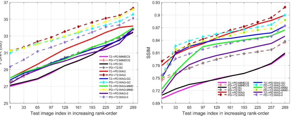
Fig. 3. Cross-modality synthesis results: MIMECS, SC, WAG, WAG-MMD, WAG-GC and WAG-0 on the IXI dataset.

TABLE II

PSNRS ANDSSIMS OF THEWAG-SYNTHESIZED IMAGES RESULTING FROM DIFFERENT PAIRED/FULL SET RATIOS DURING DICTIONARY TRAINING.

IXI Dataset

Metric (mean) _T2w Scenario #1 Scenario #2 Scenario #3 Scenario #4

7→PDw PDw7→T2w T2w7→PDw PDw7→T2w T2w7→PDw PDw7→T2w T2w7→PDw PDw7→T2w

PSNR (dB) 32.11 34.46 31.97 34.27 31.68 34.02 31.54 33.73

SSIM 0.8551 0.8602 0.8539 0.8589 0.8527 0.8578 0.8506 0.8549

TABLE III

ERROR MEASURES OF THEWAG-SYNTHESIZED IMAGES RESULTING FROM DIFFERENT PAIRED/FULL SET RATIOS DURING DICTIONARY TRAINING.

Metric (mean)

Fixing the number of paired data as 145

no unpaired data 36 unpaired data 48 unpaired data 72 unpaired data T2w7→_{PDw PDw}7→_{T2w T2w}7→_{PDw PDw}7→_{T2w T2w}7→_{PDw PDw}7→_{T2w T2w}7→_{PDw PDw}7→_T2w

PSNR (dB) 31.58 33.88 31.60 33.97 31.71 34.04 31.97 34.27

SSIM 0.8514 0.8563 0.8519 0.8570 0.8528 0.8580 0.8539 0.8589

TABLE IV

ERROR MEASURES OF THEWAG-SYNTHESIZED IMAGES RESULTING FROM DIFFERENT PAIRED/FULL SET RATIOS DURING DICTIONARY TRAINING.

Metric (mean)

Fixing the number of unpaired data as 72

37 paired data 73 paired data 145 paired data

T2w7→_{PDw PDw}7→_{T2w T2w}7→_{PDw PDw}7→_{T2w T2w}7→_{PDw PDw}7→_T2w

PSNR (dB) 31.35 33.54 31.57 33.86 31.97 34.27

SSIM 0.8487 0.8532 0.8514 0.8560 0.8539 0.8589

• WAG-MMD: WAG using MMD regularization only • WAG-GC: WAG using Geometric Co-regularization only • WAG: Fully fledged WAG method

In particular, SC can be cast as a fundamental baseline only considering the joint dictionary learning. MIMECS, Ve-S and Ve-US are the most relevant and state-of-the-art cross-modality image synthesis approaches. We consider three special cases of the proposed method by excluding all regularization terms (WAG-0) or including only either MMD term (WAG-MMD) or geometric co-regularization term (WAG-GC) for proving that each of the added term is useful for more accurate synthesis. The mathematical models of WAG-MMD and WAG-GC are provided in Section III-D3 and III-D4, respectively.

D. Experimental Results

T2

T2ww GGrorouunndd TTrurutthh (P

(PSSNNR R (d(dB),B), SSSSIMIM)) T

1

T1w SC

(26.33, 0.7286) SC (26.33, 0.7286)

MIMECS (26.69, 0.7505)

MIMECS (26.69, 0.7505)

V_US (27.76, 0.8281)

V_US (27.76, 0.8281)

V_S (28.07, 0.8295)

V_S (28.07, 0.8295)

WAG (28.69, 0.8603)

[image:11.612.52.564.209.410.2]

WAG (28.69, 0.8603)

Fig. 4. Example cross-modality synthesis results generated by MIMECS, SC, Ve-S Ve-US and WAG on the NAMIC dataset.

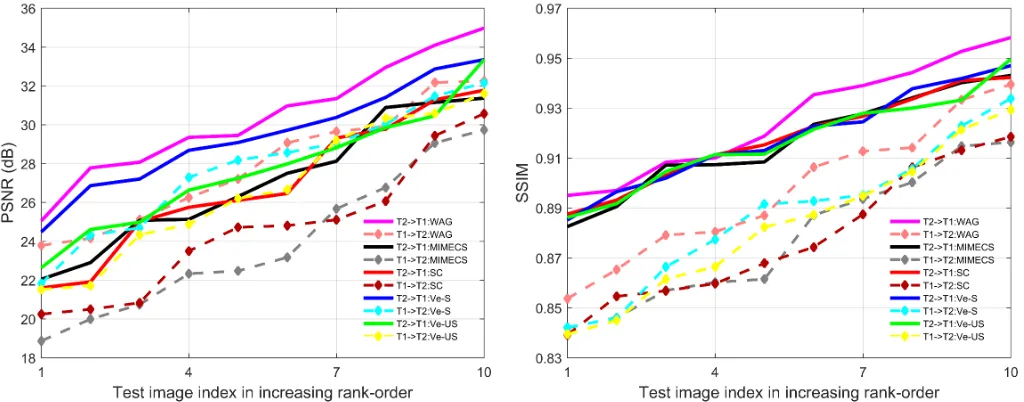
Fig. 5. Cross-modality synthesis results: MIMECS, SC, WAG, Ve-S and Ve-US on the NAMIC dataset.

TABLE V

AVERAGEDPSNRS ANDSSIMS OF THE SYNTHESIZED IMAGES USING DIFFERENT METHODS ON THENAMICDATASET.

NAMIC Dataset

Metric (mean) T1w7→T2w T2w7→T1w

MIMECS SC Ve-US Ve-S WAG MIMECS SC Ve-US Ve-S WAG PSNR (dB) 23.88 24.58 26.70 27.76 27.96 27.05 26.90 27.66 29.40 30.40

SSIM 0.8779 0.8778 0.8832 0.8874 0.8991 0.9165 0.9177 0.9168 0.9182 0.9259

subjects leads to better synthesis results. The proposed method under the weakly coupled settings (i.e.small number of paired images in scenario #4) can match the performance of fully coupled method (in scenario #1) for cross-modality synthesis. To see the impact of the number of registered image pairs or unpaired data in WAG, in Tables III and IV, we show the mean performance of our proposed method based on different ratios of paired and unpaired data. In those results, we first fix the number of registered image pairs to be 145 (referring to scenario #2) to observe the performance variation by increasing the number of unpaired data from 36 to 72. Generally, more unpaired data yield better results. We evaluate how the number of paired data influences the synthesized results given the fixed number of unpaired images as 72. The number of paired images is set to 37, 73 and 145 (the same sets in scenario #2-#4). The more existing paired data, the

better the synthesized results.

In the second scenario, we evaluate WAG and other relevant methods on the NAMIC dataset involving two sets of major experiments. The representative and stat-of-the-art synthesis methods, including SC, MIMECS, Ve-S and Ve-US are em-ployed to compare with our WAG model. We demonstrate visual and quantitative results in Fig. 4, Fig. 5 and summarize the averaged values in Table V, respectively. It can be seen that our method yields the best results against the compared approaches proving our claim of being able to synthesize better results through the added two regularization terms under weakly-supervised setting.

[image:11.612.71.543.472.528.2]

TABLE VI

PAIRED T-TEST ON THEWAGIMPROVEMENTS USING THEIXIDATASET.

Paired t-test WAG vs. WAG-0 WAG vs. WAG-MMD WAG vs. WAG-GC IXI: T2w7→_PDw

p-value (PSNR) <0.001 <0.001 <0.001

p-value (SSIM) <0.001 <0.001 <0.001

IXI: PDw7→_T2w

p-value (PSNR) <0.001 <0.001 <0.001

p-value (SSIM) <0.001 <0.001 <0.001

TABLE VII

INDEPENDENT T-TEST ON THE PERFORMANCE BENEFITS USING THEIXIDATASET.

Independent t-test WAG vs. MIMECS WAG vs. SC IXI: T2w7→PDw

p-value (PSNR) <0.001 <0.001

p-value (SSIM) <0.001 <0.001

IXI: PDw7→_T2w

p-value (PSNR) <0.001 <0.001

p-value (SSIM) <0.001 <0.001

TABLE VIII

INDEPENDENT T-TEST ON THE PERFORMANCE BENEFITS USING THENAMICDATASET.

Independent t-test WAG vs. MIMECS WAG vs. SC WAG vs. Ve-US WAG vs. Ve-S NAMIC: T1w7→_T2w

p-value (PSNR) 0.0319 0.0308 0.0450 0.0363 p-value (SSIM) 0.0347 0.0396 0.0468 0.0392

NAMIC: T2w7→T1w

p-value (PSNR) 0.0168 0.0361 0.0809 0.041 p-value (SSIM) 0.0143 0.0138 0.0464 0.0345

for the synthesis of one 3D representative image with size 256×256×100 pixels took about 7 minutes.

E. Statistical Test

We conduct two statistical tests illustrating the significance of the improvements introduced by (1) the various regulariza-tion terms within WAG, and (2) our method compared with other state-of-the-art approaches. Regarding the characteristics of the comparison, we employ a paired-sample t-test for group (1) and independent (two-samples) t-test for group (2) at 5% significance level. Table VI lists the results of paired t-test for case (1), which shows our improvements are all statistically significant. Tables VII and VIII show the results of independent t-test for case (2), which demonstrates that the performance benefits of our method against others are statistically significant in all but one case, i.e., synthesizing T1w images from T2w data on the NAMIC dataset using Ve-S method.

V. DISCUSSIONS

To investigate the performance of the proposed method, in this paper, we extensively validated WAG on two public datasets, i.e., IXI and NAMIC. We compared our results with other state-of-the-art methods for cross-modality image synthesis. We illustrated our method on different synthesis scenarios of structural brain MRI and synthesized images of both healthy and schizophrenic subjects. A few registered

supervised state-of-the-art methods under a weakly-supervised setting (with only 12.8% registered data) in both healthy and pathological scenarios. This reveals its capability in effectively leveraging data to boost the learning system. Therefore, the proposed method is usable in clinical practice considering the fact that collecting parallel image pairs is costly and usually limited in many situations.

WAG achieves compelling synthesis results in this paper for the specific MRI modalities investigated here. However, our method could be potentially applied to other imaging modalities having the assumption that images with similar high order edge/texture characteristics and resolutions. It remains to be demonstrated the synthesis quality in more complex settings like, for instance, for the synthesis of PET images from MRI data, for the synthesis of MRI data from CT images, and for the more challenging cases such as the synthesis of a tumor case. In addition, to address multi-modality image synthesis involving more than two modalities, the natural extension of the proposed method would currently required that all source modalities would be available at once at the input. We are aware of very recent work by other researchers that handle multi-modality image synthesis even in the absence of one of some source modalities [44]. In our future work, we plan to explore extensions to our framework based on multi-modality image fusion of the source modalities before the synthesis. Fused features can better express multiple source modalities and thus synthesize the target image modality even with only partial input sources.

VI. CONCLUSION

We proposed a weakly-coupled and geometry co-regularized joint dictionary learning (WAG) method for cross-modality synthesis of MRI images. Most conventional joint dictio-nary learning methods with sparse representations assume a fully supervised setting. Instead, our method only requires a small subset of registered image pairs and automatically finds correspondences for a much larger set of unpaired images. This process assists and enriches the supervised learning on the smaller subset while booting synthesis performance. With the proposed cross-modality image matching criterion, the derived common feature space associates cross-modality data effectively by updating a pair of dictionaries in both domains. We integrated our model with both MMD and modality-specific geometric co-regularization terms to further improve image synthesis quality. The proposed WAG approach was applied to cross-modality image synthesis of brain MRI and experimental results demonstrated that WAG significantly outperforms competing state-of-the-art methods on two public databases with healthy and schizophrenic subjects.

REFERENCES

[1] G. van Tulder and M. de Bruijne, “Why does synthesized data improve multi-sequence classification?” in Inter-national Conference on Medical Image Computing and Computer-Assisted Intervention. Springer, 2015, pp. 531–538.

[2] L. G. Ny´ul, J. K. Udupaet al., “On standardizing the mr image intensity scale,”image, vol. 1081, 1999.

[3] A. Madabhushi and J. K. Udupa, “New methods of mr image intensity standardization via generalized scale,”

Medical Physics, vol. 33, no. 9, pp. 3426–3434, 2006. [4] S. Roy, A. Carass, and J. L. Prince, “Magnetic resonance

image example-based contrast synthesis,” IEEE Trans. Med. Imaging, vol. 32, no. 12, pp. 2348–2363, 2013. [5] Y. Huang, L. Beltrachini, L. Shao, and A. F. Frangi,

“Geometry regularized joint dictionary learning for cross-modality image synthesis in magnetic resonance imag-ing,” in International Workshop on Simulation and Syn-thesis in Medical Imaging. Springer, 2016, pp. 118–126. [6] T. Cao, C. Zach, S. Modla, D. Powell, K. Czymmek, and M. Niethammer, “Multi-modal registration for correlative microscopy using image analogies,” Med. Image Anal., vol. 18, no. 6, pp. 914–926, 2014.

[7] J. Woo, M. Stone, and J. L. Prince, “Multimodal registra-tion via mutual informaregistra-tion incorporating geometric and spatial context,” IEEE Trans. Image Process., vol. 24, no. 2, pp. 757–769, 2015.

[8] J. E. Iglesias and M. R. Sabuncu, “Multi-atlas segmenta-tion of biomedical images: a survey,”Med. Image Anal., vol. 24, no. 1, pp. 205–219, 2015.

[9] N. Cordier, H. Delingette, M. Lˆe, and N. Ayache, “Extended modality propagation: Image synthesis of pathological cases,”IEEE Trans. Med. Imaging, vol. 35, no. 12, pp. 2598–2608, 2016.

[10] S. K. W. Olivier Commowick and G. Malandain, “Using Frankensteins creature paradigm to build a patient spe-cific atlas,” in MICCAI. Springer, 2009, pp. 993–1000. [11] A. Hertzmann, C. E. Jacobs, N. Oliver, B. Curless, and D. H. Salesin, “Image analogies,” in ACM SIGGRAPH, 2001, pp. 327–340.

[12] Z. Liu, Z. Zhang, and Y. Shan, “Image-based surface detail transfer,” IEEE Comput. Graphics Appl., vol. 24, no. 3, pp. 30–35, 2004.

[13] A. Jog, A. Carass, S. Roy, D. L. Pham, and J. L. Prince, “Random forest regression for magnetic resonance image synthesis,”Med. Image Anal., vol. 35, pp. 475–488, 2017. [14] D. H. Ye, D. Zikic, B. Glocker, A. Criminisi, and E. Konukoglu, “Modality propagation: coherent synthesis of subject-specific scans with data-driven regularization,” inMICCAI. Springer, 2013, pp. 606–613.

[15] R. Vemulapalli, H. Van Nguyen, and S. Kevin Zhou, “Unsupervised cross-modal synthesis of subject-specific scans,” inIEEE ICCV, 2015, pp. 630–638.

[16] N. Burgos, M. J. Cardoso, K. Thielemans, M. Modat, S. Pedemonte, J. Dickson, A. Barnes, R. Ahmed, C. J. Mahoney, J. M. Schott et al., “Attenuation correction synthesis for hybrid pet-mr scanners: application to brain studies,”IEEE Trans. Med. Imaging, vol. 33, no. 12, pp. 2332–2341, 2014.

[17] H. Van Nguyen, K. Zhou, and R. Vemulapalli, “Cross-domain synthesis of medical images using efficient location-sensitive deep network,” inMICCAI. Springer, 2015, pp. 677–684.

transfor-mation in demon registration,” in IEEE ISBI. IEEE, 2009, pp. 963–966.

[19] J. Yang, J. Wright, T. S. Huang, and Y. Ma, “Image super-resolution via sparse representation,”IEEE Trans. Image Process., vol. 19, no. 11, pp. 2861–2873, 2010.

[20] Y. Huang, L. Shao, and A. F. Frangi, “Simultaneous super-resolution and cross-modality synthesis of 3D med-ical images using weakly-supervised joint convolutional sparse coding,” inIEEE CVPR, July 2017.

[21] M. Aharon, M. Elad, and A. Bruckstein, “K-SVD: An algorithm for designing overcomplete dictionaries for sparse representation,”IEEE Trans. Signal Process., vol. 54, no. 11, pp. 4311–4322, 2006.

[22] G. Davis, S. Mallat, and M. Avellaneda, “Adaptive greedy approximations,” Constructive approximation, vol. 13, no. 1, pp. 57–98, 1997.

[23] S. S. Chen, D. L. Donoho, and M. A. Saunders, “Atomic decomposition by basis pursuit,” SIAM Rev., vol. 43, no. 1, pp. 129–159, 2001.

[24] H. Lee, A. Battle, R. Raina, and A. Y. Ng, “Efficient sparse coding algorithms,” inNIPS, 2006, pp. 801–808. [25] R. Tibshirani, “Regression shrinkage and selection via the lasso,”J. R. Stat. Soc. Series B Stat. Methodol., pp. 267–288, 1996.

[26] J. Mairal, M. Elad, and G. Sapiro, “Sparse representation for color image restoration,”IEEE Trans. Image Process., vol. 17, no. 1, pp. 53–69, 2008.

[27] H. Chang, D.-Y. Yeung, and Y. Xiong, “Super-resolution through neighbor embedding,” inIEEE CVPR.

[28] Y. Huang, F. Zhu, L. Shao, and A. F. Frangi, “Color object recognition via cross-domain learning on RGB-D images,” inIEEE ICRA, 2016, pp. 1672–1677.

[29] F. Zheng, Y. Tang, and L. Shao, “Hetero-manifold regu-larisation for cross-modal hashing,”IEEE Trans. Pattern Anal. Mach. Intell., 2016.

[30] F. Zhu and L. Shao, “Weakly-supervised cross-domain dictionary learning for visual recognition,” Int. J. Com-put. Vision, vol. 109, no. 1-2, pp. 42–59, 2014.

[31] S. Wang, L. Zhang, Y. Liang, and Q. Pan, “Semi-coupled dictionary learning with applications to image super-resolution and photo-sketch synthesis,” inIEEE CVPR, 2012, pp. 2216–2223.

[32] D.-A. Huang and Y.-C. Frank Wang, “Coupled dictionary and feature space learning with applications to cross-domain image synthesis and recognition,” inIEEE ICCV, 2013, pp. 2496–2503.

[33] A. Gretton, K. M. Borgwardt, M. J. Rasch, B. Sch¨olkopf, and A. Smola, “A kernel two-sample test,” J. Mach. Learn. Res., vol. 13, no. Mar, pp. 723–773, 2012. [34] K. M. Borgwardt, A. Gretton, M. J. Rasch, H.-P. Kriegel,

B. Sch¨olkopf, and A. J. Smola, “Integrating structured biological data by kernel maximum mean discrepancy,”

Bioinformatics, vol. 22, no. 14, pp. e49–e57, 2006. [35] M. Long, J. Wang, G. Ding, D. Shen, and Q. Yang,

“Transfer learning with graph co-regularization,” IEEE Trans. Knowl. Data Eng., vol. 26.

[36] I. Steinwart, “On the influence of the kernel on the consistency of support vector machines,”J. Mach. Learn.

Res., vol. 2, no. Nov, pp. 67–93, 2001.

[37] X. Lu, H. Yuan, P. Yan, Y. Yuan, and X. Li, “Geom-etry constrained sparse coding for single image super-resolution,” in IEEE CVPR, 2012, pp. 1648–1655. [38] M. Zheng, J. Bu, C. Chen, C. Wang, L. Zhang, G. Qiu,

and D. Cai, “Graph regularized sparse coding for image representation,” IEEE Trans. Image Process., vol. 20, no. 5, pp. 1327–1336, 2011.

[39] M. Belkin and P. Niyogi, “Laplacian eigenmaps and spectral techniques for embedding and clustering,” in

NIPS, vol. 14, no. 14, 2001, pp. 585–591.

[40] M. Long, G. Ding, J. Wang, J. Sun, Y. Guo, and P. S. Yu, “Transfer sparse coding for robust image representation,” inIEEE CVPR, 2013, pp. 407–414.

[41] H. Lee, A. Battle, R. Raina, and A. Y. Ng, “Efficient sparse coding algorithms,”NIPS, vol. 19, p. 801, 2007. [42] S. Boyd and L. Vandenberghe, Convex optimization.

Cambridge university press, 2004.

[43] Z. Wang, A. C. Bovik, H. R. Sheikh, and E. P. Simoncelli, “Image quality assessment: from error visibility to struc-tural similarity,” IEEE Trans. Image Process., vol. 13, no. 4, pp. 600–612, 2004.