Buoyancy-driven Magnetohydrodynamic Waves

BUOYANCY-DRIVEN MAGNETOHYDRODYNAMIC WAVES

A. Hague1and R. Erdélyi1,2 1

Solar Physics and Space Plasma Research Centre, School of Mathematics and Statistics, University of Sheffield, Hicks Building, Hounsfield Road, Sheffield, S3 7RH, UK

2

Debrecen Heliophysical Observatory(DHO), Konkoly Astronomical Institute, Research Centre for Astronomy and Earth Sciences, Hungarian Academy of Sciences(HAS), Debrecen, P.O. Box 30, H-4010, Hungary

Received 2016 March 17; revised 2016 May 31; accepted 2016 July 5; published 2016 September 7

ABSTRACT

Turbulent motions close to the visible solar surface may generate low-frequency internal gravity waves (IGWs) that propagate through the lower solar atmosphere. Magnetic activity is ubiquitous throughout the solar atmosphere, so it is expected that the behavior of IGWs is to be affected. In this article we investigate the role of an equilibrium magnetic field on propagating and standing buoyancy oscillations in a gravitationally stratified medium. We assume that this background magneticfield is parallel to the direction of gravitational stratification. It is known that when the equilibrium magneticfield is weak and the background is isothermal, the frequencies of standing IGWs are sensitive to the presence of magnetism. Here, we generalize this result to the case of a slowly varying temperature. To do this, we make use of the Boussinesq approximation. A comparison between the hydrodynamic and magnetohydrodynamic cases allows us to deduce the effects due to a magneticfield. It is shown that the frequency of IGWs may depart significantly from the Brunt–Väisälä frequency, even for a weak magnetic field. The mathematical techniques applied here give a clearer picture of the wave mode identification, which has previously been misinterpreted. An observational test is urged to validate the theoretical findings.

Key words:hydrodynamics –magnetohydrodynamics (MHD)– Sun: atmosphere– Sun: oscillations– waves

1. INTRODUCTION

Hydrodynamic waves in a gravitationally stratified, com-pressible medium have been well studied. In addition to the gravitationally modified acoustic wave (Lamb 1932), where pressure is the primary restoring force, there are also internal gravity, or buoyancy, waves (see e.g., Lighthill 1978). In stars like the Sun, global internal oscillations(standing modes of the entire stellar interior) are known as p- and g-modes

(Cowling1941)depending on the main driving force: pressure or buoyancy.

Most of our knowledge of the Sun’s interior comes from the study of p-modes (see, e.g., Christensen-Dalsgaard 2002), while g-modes have yet to be convincingly observed (see Appourchaux et al.2010). Acoustic and internal gravity waves

(IGWs)are, however, also supported by the solar atmosphere, where they are sometimes known as atmospheric p- and g-modes. In contrast to interiorg-modes, atmospheric IGWs have already been observed by, e.g., Komm et al. (1991), Stodilka

(2008), and Straus et al.(2008). However, given the nature and purpose of these observations, they are not in the format to make direct magnetoseismic analysis, although they are strong motivations.

IGWs may be generated by convective motion in the solar sub-surface convection region. Numerical simulations by Brun et al.(2013)have shown that internalg-modes may be excited in the solar radiative interior by turbulent convection. Atmo-spheric IGWs in the solar atmosphere may also be excited in a similar fashion, as suggested by Komm et al.(1991).

Among the many differences, one major difference between the solar interior and atmosphere is the presence and potential role of magnetism. The solar atmosphere is permeated by magnetic fields, which play a vital role in structuring the atmosphere and in the dynamics of atmospheric plasma. Often, we must use a magnetohydrodynamic (MHD) description of solar plasmas in the presence of a magnetic field. It is well

known that a magnetic field has significant implications for helioseismology; see, e.g., the reviews by Thompson (2006) and Erdélyi (2006a,2006b). The details of how the magnetic field affects the properties (e.g., frequency, amplitude, polarization, reflection or refraction, etc.)of acoustic or internal gravity modes is a fundamental question. Once it is known how these changes scale with the presence of a magneticfield, wave measurements may be inverted to deduce information about the magnetic field itself. This is a relatively new area of solar physics, and is referred to as solar magneto-seismology when applied to diagnostics.

The frequencies ofp-modes are seen to vary with the solar cycle. Chaplin et al. (2007) used data taken over three solar cycles to analyze changes top-mode frequencies due to these cycles. These are global oscillations affected by variations to the overall magneticfield of the Sun. However, local magnetic fields are also important.p-modes are reported to be damped when propagating through a sunspot(Braun et al.1987, just to name a widely studied example). The effect of a vertical magnetic field on p-modes has been investigated analytically by, e.g., Zhugzhda & Dzhalilov(1981,1982), Spruit & Bogdan

(1992), Cally & Bogdan(1993), Cally et al.(1994), Hindman et al.(1996), and Jain et al.(2009).

The theory of MHD waves and oscillations in stratified medium, in which the magneticfield is parallel to gravity, has also been developed by, e.g., Ferraro & Plumpton (1958), Syrovatskii & Zhugzhda (1968), Hollweg (1979), Zhugzhda

(1979), Leroy & Schwartz (1982), Schwartz & Leroy(1982), Zhugzhda & Dzhalilov (1984a), Moreno-Insertis & Spruit

(1989), Hasan & Christensen-Dalsgaard(1992), Cally(2001), Roberts (2006), and recently by Mather & Erdélyi (2016). Some of these works focused on the effect of a magneticfield on convection, the unstable counterpart of buoyancy oscilla-tions. One key result is that a sufficiently strong magneticfield can inhibit convection, i.e., wave propagation may be possible when the square of the Brunt–Väisälä frequency is negative.

A horizontal magneticfield was analyzed in the Boussinesq approximation by Barnes et al. (1998). It was shown that propagating IGWs have a buoyancy and a magnetic component in an MHD model. In the presence of a vertical magneticfield the picture is less clear. The slow and fast MHD waves have mixed properties and mode conversion can occur when the sound and Alfvén speeds are equal. For a treatment of mode conversion see, e.g., Zhugzhda & Dzhalilov (1982)and Cally

(2001, 2006). This phenomenon makes the mathematical treatment of MHD waves in this model, i.e., with a vertical equilibrium magneticfield, very difficult. The coupled second-order governing equations were first derived by Ferraro & Plumpton(1958). Exact solutions of this system, for the case of a constant background temperature, were found by Zhugzhda

(1979) in terms of Meijer G-functions (or equivalently hypergeometric functions, as shown by Cally 2001). Exact solutions for more complicated background states are not yet known. For large horizontal wavenumbers, the slow wave is, to an extent, decoupled from the fast wave. The governing equation for the slow wave when this is the case, derived by Roberts (2006), is of Klein–Gordon form. Solutions for an isothermal background have been investigated by, e.g., Hasan & Christensen-Dalsgaard (1992).

It is important to understand the wave processes in the solar atmosphere. There is plenty of evidence that the solar atmosphere contains structures that may be modeled as stratified plasma embedded in vertical magneticfields. MHD waves in such structures (when stratification is along the magnetic field) are difficult to analyze. To gain some under-standing of the situation we focus on MHD waves that are more applicable to the lower solar atmosphere, where buoyancy may play a key role. The knowledge gained from such a model will allow us to measure and explain dynamic processes in the solar atmosphere.

It was shown by Straus et al. (2008) that IGWs are suppressed by a strong magnetic field. In this work we shall restrict our attention to a weak magneticfield to determine the nature of IGWs in a magnetic environment. We aim to establish how the properties (e.g., frequency) of IGWs are affected by the presence of a magneticfield. In particular, we aim to gain insight into how these changes(if any)scale with the magnetic field. Knowing such scaling may ultimately allow us to develop inversion techniques to determine the magneticfield present in such waveguides.

To study IGWs analytically, we apply the Boussinesq approximation. Wefirst consider the purely hydrodynamic case of no magneticfield. This approach is applicable to the lower solar atmosphere in regions with very little magnetic activity. We should note, however, that what may appear to be afi eld-free region with some instruments may actually contain many small-scale magnetic features. We examine both propagating and standing waves. After considering the hydrodynamic problem, we move onto the MHD case. We address IGWs from the viewpoint of MHD waves and determine the introduced changes in frequency due to the presence of a vertical equilibrium magneticfield. A vertical magneticfield is directly applicable to localized structuring phenomena such as sunspots, pores, and coronal holes. It has also been shown by Reardon et al. (2011) that chromospheric fibrils, previously thought to predominantly be horizontal fields, instead have much “more”vertical than horizontal magnetic flux; this is a potential new application with the caveat that these features are

rather dynamic(i.e., time-dependent), therefore caution has to be exercised not to over-interpret.

The approximations used in this analysis lend themselves to the lower solar atmosphere, specifically the photosphere or low chromosphere(where the plasma-βcould still be large in local magnetic structures, even for strong magnetic fields). In this region, we expect IGWs to be generated by convective motion and be influenced by the magnetic structures permeating the solar atmosphere. The conditions of the solar chromosphere may lead to some trapping of IGWs. A vertical magneticfield may then be used to model the chromosphere. Paralleling the case of a horizontal field, we shall see that under the assumptions we make in this article, the oscillations considered here are slow magnetoacoustic-gravity(MAG)waves.

2. A FIELD-FREE ATMOSPHERE

Let us consider the hydrodynamic case of no magneticfield, applicable to the QS. We employ linear perturbations in afluid stratified by gravity. The spherical nature of the Sun is neglected and we use a Cartesian coordinate system(x y z, , ), applicable to large horizontal wavenumbers, i.e., the l of perturbations in a spherical system is large (Pintér 1999). Gravity acts in the negative z-direction, g =(0, 0, -g).The background density and pressure depend on height only,

r r

= =

p₀ p z₀( ), _{0 0}( )z . There are no background flows,

=

v0 0.The background state is in hydrostatic equilibrium,

r

= -dp

dz g , 1

0

0 ( )

and satisfies the equation of state,

r

= 

p k

m T, 2

0 B

0 0 ( )

where kB is Boltzmann’s constant, T0 is the background temperature, and m is the mean particle mass. Around this static background we take small (i.e., linear), adiabatic, perturbations of the governing equations.

To study IGWs, uncoupled from sound waves, we apply a Boussinesq-type approximation. Essentially, perturbations to the density are significant only when multiplied by the acceleration due to gravity g, i.e., when a buoyancy force is acting. In the Boussinesq-type approximation, the linearized governing equations (where we also apply the Cowling approximation)are

r

· ( 0 1v)=0, ( )3

r ¶  r

¶ = - +

v

g

t p , 4

0 1

1 1 ( )

r

r

¶ ¶t =

N

g vz, 5

1 2

0 1 ( )

whereNis the Brunt–Väisälä frequency defined by ⎛

⎝

⎜ ⎞

⎠ ⎟

r r

= = - +

N N z g

z

d z

dz g

c

1

, 6

s

2 2

0 0

2

( )

( ) ( )

( )

where cs is the (adiabatic) sound speed given by

g r

=

velocityfield( ·v1=0), applicable to a medium where the

density may be considered constant, however, we follow Lighthill(1978). This is sometimes referred to as the anelastic approximation. This approximation is more suited to the solar atmosphere, where the density may vary significantly.

The Boussinesq approximation may be used to study buoyancy-driven waves when the wavenumber of the perturba-tions is large compared to both N2 g _{and g c ,}

s

2 _{see, e.g.,}

Lighthill(1978). Note that

r r

+ =

-N

g g

c

d

dz

1

. 7

s 2

2

0 0

( )

The terms neglected from the governing equations in the Boussinesq approximation relate to the compressibility of the plasma and contribute to the generation of acoustic waves. In applying the Boussinesq approximation, we are therefore making an assumption based on the wavelength of the waves rather than the state of the medium. For more on the applicability of the Boussinesq approximation, see, e.g., Spiegel & Veronis(1960).

We may form a single equation from Equations(3)to(5), in terms of the vertical component of momentum q=r0 1vz, by

taking the y-component of the curl of Equation (4) and eliminating v1xandr1,

 ¶

¶ =

-¶ ¶ q

t x N q. 8

2 2

2

2

2

2 _{( )}

Note that we assume no y-dependence, without loss of generality, as there is no preferred horizontal direction. Equation (8) is the governing equation for IGWs in the Boussinesq approximation. In deriving Equation (8), the y-component of the vorticity equation was employed, and the x-and z-components do not correspond to interesting physics in the present context.

We may assume normal modes in Equation (8), that is, assume q is proportional to exp(ik xx -i tw ). The governing

equation then takes the form ⎛ ⎝

⎜ _w ⎞_⎠⎟

=

-d q

dz k

N q

1 . 9

x 2

2

2 2

2 ( )

We shall investigate Equation (9) in the context of both propagating and standing waves.

2.1. Propagating Waves

Assuming that the equilibrium quantities r₀ and p0change slowly with height, we can apply the WKB method(see, e.g., Bender & Orszag 1978) to obtain a local dispersion relation. First, we introduce a slowly varying spatial variable z˜=z, where1,and assumeq takes the form

⎜ ⎟

⎛ ⎝q ⎞⎠

=

q w z( ˜)exp i ( ˜)z . (10)

Substituting Equation (10) into (9) and keeping the leading order terms(i.e., terms order₍0_{))we are left with}

⎜ ⎟

⎡ ⎣

⎢⎛_⎝⎜ ⎞_⎠⎟ ⎛ ⎝

⎜ ⎞_⎠⎟⎤

⎦

⎥ ⎛_⎝ ⎞_⎠



q

w q

+ - =

d

dz k

N

w z i z

1 exp 0. 11

x 2

2 2

2

˜ ( ˜) ( ˜) ( )

Noting that the local vertical wavenumber is given by

q

= 

kz d dz, wefind the local dispersion relation

w =

+ k

k k N . 12

x

x z

2

2

2 2

2 _{( )}

This is the well-known dispersion relation for IGWs ( Light-hill 1978). The Brunt–Väisälä frequency is then the upper cutoff frequency of IGWs. Whenkxis large in comparison to

kz, w2»N2.This agrees with the result that a plasma element displaced vertically from equilibrium will be restored by buoyancy and undergo simple harmonic motion at the Brunt– Väisälä frequency.

2.2. Standing Waves

The Brunt–Väisälä frequency changes significantly through-out the solar chromosphere(see e.g., Newington & Cally2010). This may cause the trapping of IGWs in the solar photosphere, leading to a cavity in which standing modes may form. We should therefore not restrict ourselves to propagating modes only and consider these standing modes. Furthermore, standing modes are excellent tools for carrying out solar magneto-seismology. Deriving diagnostic information from inverting changes, e.g., in the frequency or node/anti-node positions caused by inhomogeneity, structuring, or even time-depend-ence of the waveguide, are popular applications in solar physics. Although there is an extensive literature detailing how to make such applications by means of MHD waves(e.g., slow sausage, fast kink, or even Alfvén), there is limited work on IGWs in this context.

We now consider standing waves and thus must solve (9) with appropriate boundary conditions. Standing waves may occur in the solar atmosphere due to turning points or reflection by, e.g., a sharp change in phase speeds caused e.g., by sharp changes in, for example, temperature. LetLbe the length of the cavity, zÎ -[ L, 0]. Let us consider the case that the background temperature varies linearly withz,

⎛ ⎝

⎜ ⎞_⎠⎟

= 

-T T z

z

1 13

0 0

0

( )

where T0 is the temperature at z=0 and z0(>0) is the

temperature scale height. The temperature, pressure, and density are related by the equation of state, Equation (2). Using Equation(13)together with Equations(1)and(2)has the consequence that the density and pressure profiles are given by

⎛ ⎝

⎜ ⎞_⎠⎟ ⎛_⎝⎜ ⎞_⎠⎟

r =r - =

-+

 

z z

z p z p

z z

1 , 1 , 14

m m

0 0

0

0 0

0 1

( ) ( ) ( )

wherer₀ and p₀ are positive constants and represent density and pressure in the limitz0, andmis a constant known as the polytropic index. Equation (1) implies that

g

=

-m z g0 cs2( )0 1. We note that pressure and density are related by

r

= +

p0 K 0 m, 15

1 1

( )

Väisälä frequency is given by ⎛ ⎝ ⎜ ⎞ ⎠ ⎟ ⎛ ⎝ ⎜ ⎞ ⎠ ⎟ = - =

-N N z

z N g

m z

g

c

1 , , 16

s 2 02 0 1 02 0 0

2 ( )

where N₀2 is constant (note that N₀2 can be negative). We also note that we consider a non-adiabatic polytrope, that is,

g¹1 +1 m. We study a system where the effect of buoyancy is significant, so the medium is not neutrally stable. The Schwarzschild criterion for convective stability ( Light-hill1978)implies thatm>3 2 wheng=5 3.

Exact solutions to the governing Equation (9)are available in terms of Whittaker functions. It is instructive, however, to consider the case of slowly varying temperature (which has applications to the solar atmosphere and the magnetohydro-dynamic case considered later), that is, we assumeLz0.Let

*

=

z Lz ,z*Î -[ 1, 0], then the Brunt–Väisälä frequency can be written ⎛ ⎝ ⎜ *⎞_⎠⎟ ⎛_⎝⎜ *⎞_⎠⎟ = - » + -

N N Lz

z N

Lz z

L z

1 1 as 1. 17

2 0 2 0 1 0 2 0 0 ( )

Returning to the dimensional variablez,Equation(9)with the Brunt–Väisälä given by Equation(17)leads us to

⎛ ⎝ ⎜ ⎛_⎝⎜ ⎞_⎠⎟⎞ ⎠ ⎟ w = - + d q dz k N z z q

1 1 . 18

x 2 2 2 0 2 2 0 ( )

Equation(18)has solutions of the form

= Q + Q

q C1Ai( ) C2Bi( ), (19)

where Ai and Bi are the linearly independent Airy functions

(see Abramowitz & Stegun 1972)and ⎛ ⎝ ⎜ ⎞ ⎠ ⎟ w w

Q = - +

-N k N

z N z z z

1 . 20 x 0 2 2 0 2 2 0

02 0 2 0

1 3

( ( ) ) ( )

We have solved the governing equation for q, that is, the amplitude of the waves. Let us now apply appropriate boundary conditions to determine the eigenfrequencies of the perturbations. We are considering standing waves in a cavity of lengthL. The boundaries arefixed and perfectly reflecting. The boundary conditions for such a layer are

= - =

v1z( )0 v1z( L) 0. (21)

Applying these boundary conditions to solution (19), we mayfind the dispersion relation

Q Q- - Q- Q =

Ai( 0)Bi( L) Ai( L)Bi( 0) 0, (22)

where Q Q0, -L denote Θ (Equation (20)) evaluated at

=

-z 0, L,respectively. This equation cannot be inverted for the eigenfrequencies without some further simplifications. The Boussinesq approximation is valid for large wavenumbers, hence we assume k to be large, i.e., k zx 01. This approximation is also very useful in the magnetic case. The wavenumber appears inΘof order k zx 0 ,

2 3

( ) i.e.,Θis large. An asymptotic expansion is therefore possible ifk zx 0is sufficiently

large. Let us make use of the asymptotic properties of the Airy

functions(Abramowitz & Stegun1972),

⎜ ⎟ ⎜ ⎟ ⎛ ⎝ ⎞⎠ ⎛ ⎝ ⎞⎠

p z p

p z p

- ~ +

- ~ +  ¥

-

-z z

z z z

Ai sin

4 ,

Bi cos

4 , , 23

1 2

1 4

1 2 14

( )

( ) ( )

where

z= 2z z < p

3 , and arg 2

3 . 24

3

2 ∣ ∣ ( )

Letting ⎛ ⎝ ⎜ ⎞ ⎠ ⎟ w w

Q = - + - = -Q~

N k N

z N z z z

1 , 25 x 0 2 2 0 2 2 0 0 2

0 2 0

1 3

( ( ) ) ( )

we may write Equation(22)as

⎜ ⎟ ⎜ ⎟ ⎜ ⎟ ⎜ ⎟ ⎡ ⎣⎢ ⎛ ⎝ ⎞⎠ ⎛⎝ ⎞⎠ ⎛ ⎝ ⎞⎠ ⎛⎝ ⎞⎠ ⎤ ⎦⎥

p z p z p

z p z p

p z z

Q Q + +

- + +

= Q Q - =

~ ~ ~ ~ - -- -sin

4 cos 4

sin

4 cos 4

sin 0, 26

L L L L L 1 0 0 0 1 0 0 1 4 1 4 1 4 14

( ) ( )

where

z= Q2~

3 . 27

3

2 _{( )}

Equation(26)implies ⎛ ⎝ ⎜ ⎞ ⎠ ⎟ ⎡⎣⎢ ⎛ ⎝ ⎜ ⎛_⎝⎜ ⎞_⎠⎟ ⎞ ⎠ ⎟ ⎤ ⎦ ⎥ ⎥ z z w w w p - = -- + - = -N k

z z N

N z L

z z n

2 3

1

1 . 28

L x 0 02 2 2 0 1 2 0 0

2 2 3₂

0 2 0 0 2 0 3 2 ( ( )) ( )

Making use of the fact thatL z01,we may Taylor-expand Equation (28) around L z0=0. Retaining the first term in

L z0,the dispersion relation becomes

w p » + k k n L

N . 29

x

x 2

2

2 2 2

2

02 ( )

A comparison to the local dispersion relation shows that the term np L acts as a vertical “wavenumber.” Equation (29) possesses the familiar anti-Sturmian behavior of IGWs, that is, the eigenfrequencies decrease asn increases. Equation(29)is convenient for estimating the eigenfrequencies, as it allows us to use the Brunt–Väisälä frequency evaluated at the top of the cavity. This is to be expected by the assumption of a slowly varying medium; this analysis, however, serves as justification. We also consider the case of constant sound speed

(isothermal background temperature). It can be shown(details omitted)that the exact expression for the eigenfrequencies is

w p = + k k n L

N , 30

x

x 2

2

2 2 2

2

as expected. It is simple to show thatN0 =N -g z ,

2 2

0 hence

the eigenfrequencies are lower for the polytropic case than the isothermal case. That is, the effect of variable temperature is to decreasethe frequency of IGWs. This feature could be rather relevant for observational validation.

We have determined the frequencies of propagating and standing IGWs using the Boussinesq approximation. Magnetic fields are ubiquitous through the solar atmosphere, as argued before, so we must now take into account their role in the dynamic processes at work as a next step. In the following section, we consider the plasma to be embedded in a vertical magnetic field.

3. A MAGNETIC ATMOSPHERE

Let us now consider magnetohydrodynamic wave propaga-tion, applicable to magnetically active localized regions such as pores and sunspots. It has already been observed that strong magnetic fields inhibit the propagation of IGWs (Straus et al. 2008). We expect, however, that the weak magnetic fields found in the solar photosphere will also have some effect on IGWs. In particular, we aim to establish whether the frequencies of IGWs, present in a plasma embedded in a magnetic field, are effected. The magneticfield is vertical and uniform,B0 =(0, 0,B0).The linearized ideal MHD governing equations, in the Cowling approximation, can be reduced to

⎛ ⎝

⎜w + + ¶ ⎞_⎠⎟x ⎛_⎝⎜ ⎞_⎠⎟ x

¶ +

¶

¶ =

-¶ ¶

¶ ¶

c v

x v z g c z x , 31

s x s

z

2 2

A 2 2

2 A

2 2 2

2

( ) ( )

⎛ ⎝

⎜w - g¶ ⎟⎞_⎠x _⎝⎜⎛ g ⎞⎟_⎠ x

¶ +

¶

¶ = -

-¶ ¶

¶ ¶ g

z cs z z g 1 cs z x , 32

x

2 2 2

2

2

( ) ( )

⎛ ⎝

⎜w + ¶ ⎞_⎠⎟x

¶ =

v

z y 0. 33

2 A 2 2

2 ( )

where x=(x x xx, y, z) is the Lagrangian displacement vector

and vA 2

is the square of the Alfvén speed defined by

mr

=

vA2 B02 0. We note there is no preferred direction in xor

yso we may assume that, without loss of generality, there is no y-dependence. If we assume plane waves in the horizontal direction, neglectingy-dependence is equivalent to rotating the coordinate system such that the wavevector is aligned with the x-axis. These equations were first derived by Ferraro & Plumpton(1958)and have been widely applied. Equations(31) and(32)govern the fast and slow MAG waves, which couple together in this model. Equation (33) shows that the Alfvén wave, driven purely by magnetic tension, is decoupled from the system.

In this article we are primarily interested in buoyancy-driven motion and hence we neglect the effect of mode coupling as a first simplification. Our goal here is to derive analytical solutions to the governing equations, which may be used when buoyancy is the primary restoring force, i.e., in the case of atmospheric g-modes. This motivates a different approach to the analysis than works focusing on mode conversion, e.g., Spruit & Bogdan(1992)and Cally & Bogdan(1993). Here, we derive the governing equation for buoyancy-driven motion where the stratified plasma is embedded in a uniform vertical magneticfield.

Instead of using the full governing equations we may now derive a governing equation, again, in the Boussinesq approximation. The linearized equations are

r

· ( 0 1v)=0, (34)

r

r

¶ ¶t =

N

g vz, 35

1 2

0 ( )

r

m r m

 

¶

¶ = - - + +

¶ ¶

v

g B

t p

B B B

z , 36

0 1

1

0 1 1

0 1

( )

 

¶

¶ =

¶

¶ - =

B v

B v B

t B z , 0. 37

1

0 1 0 · 1 · 1 ( )

We may write a single equation for the z-component of perturbed momentum, q, via the y-component of the curl of Equation(36),

⎛ ⎝

⎜ ⎞

⎠ ⎟

r

r

 ¶ 

¶ ¶

¶

-¶

¶

-¶

¶ =

v z

q

z x N q t q

1

0. 38

0 A 2 2

0

2

2

2 2

2

2 _{( )}

This is the governing equation for MHD perturbations in the Boussinesq approximation. The Boussinesq approximation has been applied to a vertical magneticfield by, e.g., McKenzie & Axford(2000), who derived a simplified form of Equation(38). We may now Fourier analyze Equation(38)inxandt,

⎛ ⎝

⎜ ⎞

⎠

⎟ ⎛

⎝

⎜ ⎞

⎠ ⎟

r

r w r r

w

+

-+ - =

v d

dz

dq dz

d q

dz v k

d dz

dq dz

k N q

1 1

0. 39

x

x 0 A

2 3 3

0

2 2

2 0 A

2 2

0

2₍ 2 2_{) ( )}

There is also another wave solution of Equations(34)–(37)— the Alfvén wave. This corresponds to thex- and z-component of the curl of the momentum equation. The governing equation for Alfvén waves is

⎛ ⎝

⎜_¶¶ - ¶ ⎞_⎠⎟

¶ =

t v z vy 0. 40

2

2 A

2 2

2 ( )

This equation is, as mentioned earlier, decoupled from Equation(39), hence in a vertical field the Alfvén wave does not couple to IGWs. This was not considered by McKenzie &

Figure 1. Plot of frequencies (41), where N0=0.03 =

- _c

s ,1 s 8kms ,-1 b=50. The solid line represents kx=10 km−1, the

dashed line represents kx=50 km−1, and the dot–dashed line represents

Axford(2000)due to a cumbersome mathematical treatment of Equations(34)–(37). Wefind that Equation(39)is not easy to solve analytically. We will now analyze Equation(39), via the WKB method, to study propagating waves.

3.1. Propagating Waves

For propagating waves we may perform a WKB analysis, as in the previous section, of Equation (39) to find the local dispersion relation

w = +

+

v k k

k k N . 41

z

x

x z

2 A 2 2

2

2 2

2 _{( )}

The frequencies are plotted in Figure1. We see that even for the case of a weak magneticfield, significant differences from the Brunt–Väisälä frequency are seen. The character of the solution may easily become magnetically dominated, the waves may therefore become high-frequency as opposed to low-frequency IGWs (although this is based on the specific values that the parameters take). The waves may be described then as slow MHD waves modified by gravity. In Figure1we see that the frequencies increase askzincreases, in contrast to the non-magnetic case. It should be noted that this is not true in general, as

w

¶

¶k =v - +

k

k k N , 42

z

x

x z

2

2 A

2

2

2 2 2 2

( ) ( )

which may be positive or negative. The local dispersion relation for Alfvén waves, found by a WKB analysis of Equation(40), is

w2=v kA z. 43

2 2

( )

Thefirst term in Equation(41)resembles the solution of an Alfvén wave and has lead to some authors labeling this wave as an Alfvén wave modified by gravity. This is not the case, as we have seen that the equation describing Alfvén waves is decoupled from the system of equations describing the wave given by the dispersion relation (41). This clarity owes to the elegance of using the components of the vorticity equation to derive the governing equations. To deduce what this wave is, in terms of the MHD spectrum, we note that the Boussinesq approximation is quasi-incompressible, i.e., sound waves propagate at infinite phase speed. In a magnetic configuration, this corresponds to the plasma-βbeing large, where the

plasma-β is defined by b=gcs 2v

2 A

2

. The slow MHD mode, in the large horizontal wavenumber limit, propagates along the magnetic field lines with the phase speed cT, where

= +

cT2 c vs2 A2 (cs2 vA2). In high-β plasma, cT »vA, hence the

first term in Equation(41)corresponds to a slow MHD mode propagating along the magneticfield lines. The absence of the fast MHD mode is due to the Boussinesq approximation, which corresponds to the phase speed of the fast wave tending toward infinity.

The implicit assumption of high-βplasma means that these results may be applied to regions of the Sun such as the upper interior or lower solar atmosphere, say the photosphere or low chromosphere. In the higher atmosphere, i.e., the solar corona, and in very strong magnetic structures in the lower atmosphere

(low-β structures)the Boussinesq approximation, and thus the previous result, are less applicable.

We have helped to clear up the picture of IGWs in an MHD setting. It is well-known that when the magnetic field is horizontal, the IGWs of hydrodynamics correspond to slow MHD waves. We have shown that this is also the case for a vertical magnetic field where some previous authors have mistakenly identified IGWs with Alfvén waves. This is important to recognize, as Alfvén and slow waves are orthogonal eigenmodes of the MHD differential operator and hence are different and independent(in linear approximation). To gain a deeper understanding of system we should acknowledge the completeness of the spectrum of eigenmodes. Furthermore, it is important to recognize the difference between the waves because they have different properties, including phase speed, group speed, polarization, capability and capacity to carry energy, capability to dissipate, etc. A key difference in terms of energy transportation is that Alfvén waves carry energy along magnetic field lines, while slow MHD waves may carry energy at an angle to the field lines. Note also the well-known property of IGWs in which the vertical components of the phase and group velocities have opposing signs; this property may or may not persist depending on the dominant character of the waves. It is simple to show this property via the vertical component of the group velocity, calculated from Equation(41). In the solar atmosphere, where the magneticfield is highly structured, these properties should be taken into account.

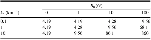
We expect to observe the waves in the lower solar atmosphere, e.g., the photosphere. In this region even plasma embedded in a strong magneticfield may be considered to be in the high-βregime. In Tables1and2we give the frequency(in mHz), determined by Equation (41), for a realistic solar atmosphere (the VAL-C model, Vernazza et al. 1981). For simplicity, we use the expression for the Brunt–Väisälä frequency in an isothermal atmosphere N2=g2 g-1 cs.

2

( )

Table1corresponds to the base of the photosphere(z»0km in the VAL-C model), where the plasma is such that the sound speed iscs»8.5kms .-1 Table2 expresses the frequencies at the top of the photosphere (z»500km), where

»

cs 6.7km s−1. Many of these frequencies are well within current instrumental capabilities. The frequency is highly dependent on the vertical wavenumber; simulation or observa-tional data is needed to determine the typical vertical

Table 1

The Frequency, Given by Equation(41), at the Base of the Photosphere

B G0( )

kz(km−1) 0 1 10 100

0.1 4.19 4.19 4.28 9.56

1 4.19 4.28 9.56 68.1

10 4.19 9.56 86.1 860

Note.The horizontal wavenumber is 1 Mm−1_.

Table 2

The Same as Table1, but Evaluated at the Top of the Photosphere

B G0( )

kz(km−1) 0 1 10 100

0.1 5.31 5.31 8.33 64.3

1 5.31 8.33 64.3 641

wavelengths of magnetic IGWs in a realistic solar atmosphere. Note that the horizontal wavenumber is taken to be 2 Mm−1, satisfying the large wavenumber criteria of the Boussinesq approximation.

Equation (41) predicts the frequencies that we expect to observe. The waves we discuss are quasi-incompressible, so intensity variations are unlikely to be of use as an identifying tool. Doppler velocities and Stokes parameters are probably the key to observing these waves. Straus et al.(2008)were able to identify IGWs in the lower solar atmosphere using line of sight Doppler velocities. These were seen using lower solar atmo-spheric lines(FeI7090, NaID1, MgIb2, NiI6764 lines)using the Interferometric Bidimensional Spectropolarimeter and Echelle spectrograph instruments at the Dunn Solar Telescope and the Michelson Doppler Imager (MDI)on board the Solar and Heliospheric Observatory (SOHO) spacecraft. In the hydrodynamic regime we expect a similar analysis to observe the waves. In the magnetic regime, this may not be applicable, as periods may be too low, although this is based on the vertical wavelength. We would suggest that a super-sensitive MDI type of instrument could pick up such signals, or using magneto-optical filters at various heights (e.g., Na D2 or the K lines, through the CaIline could also be used).

There remains the question of how to distinguish magnetic IGWs from other wave modes. There should be no confusion with acoustic or fast MHD waves, as the frequency and phase speed of such waves should be significantly different. The frequency of the magnetic IGWs (slow MHD waves)that we discuss is determined by the Alfvén frequency and the Brunt– Väisälä frequency, which are significantly less than the frequency of fast or p-modes in high-β plasma (where our results are applied, this region is the lower part of the solar atmosphere, i.e., the photosphere embedded in a magnetic field). The distinction between the magnetic IGW the Alfvén wave, may be more difficult based on instrumental capabilities but in principle is possible. The frequency of magnetic IGWs, as we have determined, is greater than the Alfvén frequency. When the magnetic field has a less determining effect, the waves may be observed as almost pure IGWs (as in Straus et al. 2008), and the magnetic effect is seen by e.g., the deviation from the frequency of IGWs. Such deviations could be observed in Dopplergrams, which are known in helioseis-mology. Unfortunately, even a weak magneticfield may cause the frequencies to become very close to the frequency of Alfvén waves. The frequency is not exactly the same, although the difference may be challenging to observe. A more significant difference may be observed in the phase and group velocities, expressions for which may be determined from Equation(41)with ease. When the waves take on a magnetic character, the distinction between Alfvén waves is in the velocity perturbations relative to the magneticfield. If one can determine the magnetic surfaces, the slow MHD waves may have velocities that are both parallel(the dominant component) and perpendicular to the magnetic field, while Alfvén waves may have velocities that are only perpendicular, within constant magnetic surfaces. In Alfvén waves the perturbations are to the magnetic and velocityfield components, so they would be out of phase. Observationally it is not easy to establish what the magnetic iso-surfaces are, but using, for example, Local Correlation Tracking, it is possible.

In this section we have confirmed that IGWs in a slowly varying medium embedded in a weak, vertical magnetic field

are slow MHD waves. The frequencies of the oscillations are modified by a term corresponding to a slow MHD wave. In the next section we will show that this is also the case for standing waves.

3.2. Standing Waves

It has been shown by Newington & Cally (2010) that a weak, vertical magneticfield has the potential to reflect upward propagating IGWs. This typically occurs below the region where the sound and Alfvén speeds are comparable. This fact, in addition to temperature variations in the low solar atmosphere may create some cavity in the photosphere/ chromosphere where IGWs are trapped, leading to standing modes in the high-β medium.

To analyze buoyancy-driven MHD standing waves, wefind it preferable to further simplify Equations(31)and(32)via the method of coordinate stretching (see, e.g., Roberts 2006), which we briefly outline here for reference. We take this approach, as the governing equation in the Boussinesq approximation is still difficult to analyze analytically. This method is equivalent to assuming small horizontal wavelength, so some analogy with the Boussinesq approximation may be drawn.

We are interested in vertical, buoyancy-driven motion, i.e., we wish to consider motion that is predominantly along the magneticfield lines. We apply the method of Roberts(2006), used to study slow MAG, which we briefly outline here (see Roberts2006for details). Let us introduce the scaling

 x x x x

= = = =

x x¯, x ¯x, z z¯, z ¯z, (44)

whereòis dimensionless and small, i.e.,1. Substituting the scaled variables into Equations (31) and (32) leaves Equation(32)unchanged but(31)becomes

⎛ ⎝

⎜ ⎞

⎠

⎟ ⎛_⎝⎜ ⎞

⎠ ⎟ 

x

w x x

+ ¶

¶ + +

¶

¶ =

-¶ ¶

¶ ¶

c v

x v z g c z x .

45

s x x s

z 2

A2 2

2

2 2 A2

2

2

2

( ) ¯

¯ ¯

¯

¯ ¯

¯ ( )

Since1, the term₍2_{)can be neglected so}

⎛ ⎝

⎜ ⎞_⎠⎟

x x

+ ¶

¶ =

-¶ ¶

¶ ¶

c v

x g c z x . 46

s

x

s

z 2

A 2 2

2

2

( ) ¯

¯ ¯

¯

¯ ( )

Equation(46)can be integrated with respect tox¯, ⎛

⎝

⎜ ⎞_⎠⎟

x

x

+ ¶

¶ =

-¶ ¶

c v

x g c z . 47

s

x

s z

2 A

2 2

( ) ¯

¯ ¯

¯ _{( )}

Let us now return to the original, unscaled variables. Elimination of¶x_x ¶x between Equations(32)and(47)leads us to

⎛ ⎝

⎜⎜ ⎛_⎝⎜ ⎞

⎠ ⎟⎞

⎠ ⎟⎟

x

g x w x

¶

¶

-¶

¶ + - + =

c

z g

c

c z

c

v N

g H

c

c 0,

48

T

z T

s

z T T

s z 2 2

2

4

4

2 2

A2 2

2

2

( )

whereH=c_s2 ggis the pressure scale height. Equation(48)is the governing equation for MHD buoyancy oscillations. This is the governing equation we shall use to investigate the slow MAG wave.

Note that if the magnetic field is absent from the model,

=

well-known dispersion relation for a fluid particle (displaced vertically from equilibrium)undergoing either simple harmonic motion due to buoyancy, or convection in the case of complex

ω. This is the dispersion relation for IGWs in the limit of large horizontal wavenumber.

Equation (48) is Equation (3.9) of Roberts (2006). This equation has also been derived previously by e.g., Moreno-Insertis & Spruit(1989)in the context of modeling convective motion in sunspots; and it was also applied by, e.g., Hasan & Christensen-Dalsgaard(1992)to study MHD waves in a high-β approximation in an isothermal atmosphere.

The scalings (44) are equivalent to assuming that the horizontal wavelength of the perturbations is small, i.e., taking the asymptotic limit k Hx  ¥.We can relate the horizontal wavenumberkxto the azimuthal orderlof spherical harmonics

(for standing waves of the entire Sun); the assumption of large wavenumber implies that l is large, that is, the analysis performed here is applicable to waves trapped close to the solar surface. Large values of lalso agree with the use of Cartesian coordinates.

Let us consider a temperature profile that increases linearly with depth, given by Equation (13). The density and pressure are given by Equation (14). The squares of the sound and Alfvén speeds take the form

⎛ ⎝

⎜ ⎞_⎠⎟ ⎛_⎝⎜ ⎞_⎠⎟

= - =

-



c c z

z v v

z z

1 , 1 , 49

s s

m

2 2

0

A2 A2

0

( )

where c_s2 and vA,

2 _{the values of sound and Alfvén speeds}

squared at z=0,are constants. The Brunt–Väisälä frequency is as in the hydrodynamic case, given by Equation(16).

A polytropic model has been considered before by, e.g., Syrovatskii & Zhugzhda (1968), Scheuer & Thomas (1981), Spruit & Bogdan(1992), Cally & Bogdan(1993), Cally et al.

(1994), and Hindman et al. (1996), although it has not been studied as extensively as an isothermal model. Many of the previous works have been motivated by oscillations in sunspots and the mode conversion of magnetically modified p-modes

(fast MHD modes)into slow MHD modes.

Let us now make the assumption of high-β plasma, in accordance with the Boussinesq approximation. A high value ofβ(i.e., a weak magneticfield)impliesv_A2 c_s2socT »v .

2 A

2

Under this assumption Equation (48)becomes

x

w x

¶

¶ + - =

v

z N 0. 50

z

z A

2 2

2

2 2

( ) ( )

This is a Sturm–Liouville type problem, in contrast to the anti-Sturmian hydrodynamic case. The Brunt–Väisälä frequency now plays the role of the lower cutoff frequency, that is, there is only wave propagation if w2>N2._{If N}2 _>w2 _{the waves}

are evanescent.

Now, substituting the expressions (49)and (16)for vA2 and N2into(50), we obtain the governing equation for longitudinal MHD wave propagation in a polytropic high-β plasma

⎡ ⎣ ⎢ ⎢

⎛ ⎝

⎜ ⎞_⎠⎟ ⎛_⎝⎜ ⎞_⎠⎟ ⎤

⎦ ⎥ ⎥

x

w x

¶

¶ + - - - =

-

v z

z

z N

z z

1 1 0. 51

z

m m

z A2

2

2 2

0

02

0 1

( )

To solve Equation(51)analytically one needs to make further simplification. We reduce the complexity of Equation (51) when the temperature varies slowly throughout the medium. In this approximation we find that the resulting governing

equation can be solved analytically, in terms of special functions.

Here, we consider standing waves in a cavity of thicknessL, i.e., zÎ -[ L, 0]. Now, we assume that the thickness of the cavity is much smaller than the temperature scale height,



L z0 (i.e., the temperature changes slowly throughout the

cavity). This assumption is relevant for a thin layer close to the solar surface, and thus complements the scaling (44) when deriving the governing equation. If we again introduce a new variable,z*, such thatz=Lz* wherez*Î -[ 1, 0 ,] we Taylor-expand the above equation for small L z0, as L z01 by

assumption. Tofirst order inL z0this is

⎡ ⎣⎢

⎤ ⎦⎥ *

*

x

w w x

¶ ¶

+ - - - - =

 v

L z

N m N m z L

z

1 0.

52

z

z A2

2 2

2

2

02 2 02

0

( ) ( ( ))

( )

Returning to the dimensional variable z in favor of z*, the solution is, again, given by Airy functions

xz=C x1( )Ai( )Q +C x2( )Bi( )Q , (53)

where ⎛ ⎝

⎜ ⎞

⎠

⎟ w w

= - -

-+ +

-

Q

v z N m m mz z

N z z m

1

1

1 .

54

A 2 0

1 3

02 2 2 3 2 0

02 0

( ( ) ) [ ( )

( ( ))]

( )

It can be shown that the solutions are spatially oscillatory for

Î

-z [ L, 0]ifw2>N

02 and m>1.

We now consider standing waves in a cavity of lengthL. We assume the boundaries of the cavity to be perfectly reflecting. As in the hydrodynamic case, reflection can occur due to an abrupt change in the background; see, e.g., Scheuer & Thomas

(1981). Slow waves may also be reflected in a region where the Alfvén and sound speeds are equal, due to mode conversion

(Zhugzhda & Dzhalilov1984b). As mentioned in the previous section, this work is restricted to the case of a weak magnetic field, hence there is no region in which mode conversion can occur.

We are considering a standing wave problem in a finite cavity with reflecting boundaries. The desired dispersion relation

- =

-

-Q Q Q Q

Ai( L)Bi( 0) Ai( 0)Bi( L) 0, (55)

whereQ0andQ-L areQ∣z=0andQ∣z=-L.

This equation is highly transcendental and cannot be solved easily for w, which appears implicitly in Q0,Q-L. We can

probe some information by noting that the parameterz0is large in comparison to L, i.e., the medium has slow temperature variation. Using the variablez*,defined earlier, we note thatQ is of the order of z0 L

2 3

( ) in the large parameter z0 L. An asymptotic expansion around large Q is therefore possible. Letting

= -~ - = -~

-Q0 Q0, Q L Q L, (56)

where, for spatially oscillating solutions, Q~ ~0,Q-L>0. The

as

⎜ ⎟ ⎜ ⎟

⎜ ⎟ ⎜ ⎟

⎛ ⎝

⎜ ⎛_⎝ ⎞_⎠ ⎛_⎝ ⎞_⎠

⎛

⎝ ⎞⎠ ⎛⎝ ⎞⎠

⎞ ⎠ ⎟

p z p z p

z p z p

p z z

+ +

- + +

= - =

~ ~

~ ~

-

--

-Q Q

Q Q

sin

4 cos 4

sin

4 cos 4

sin 0, 57

L L

L

L L

1 0

1 4 1 4 0

0

1 0

1 4 1 4 0

( ) ( )

where

z = 2Q~ z_- = Q~

-3 ,

2

3 . 58

L L

0 0

3 2 3 2

( )

Equation(57)implies ⎛

⎝

⎜ ⎞

⎠ ⎟

⎛ ⎝

⎜ ⎛

⎝

⎜ ⎞

⎠

⎟ ⎛

⎝

⎜ ⎞

⎠ ⎟⎞

⎠

⎟ ⎤

⎦ ⎥ ⎥

w w

w

p

- -

-- + - -

-=

-

v z z N m m N

mL

z N m

L

z n

2 3

1

1

1 1 1

.

59

A2 0 1 2

0 3 2

0

2 2 1 2

02 3 2

2

0 02

0 3 2

( ( ) ) [( )

( )

( )

This is an algebraic equation inω, although it still cannot be solved exactly analytically. We can, however, solve Equation(59)if we Taylor-expand around the small parameter

L z0.We retain only thefirst term inL z0.The frequencies can

then be expressed as

w = n p v +

L N . 60

2 2 2

A2

2 0

2

( )

These are asymptotic approximations of the eigenfrequencies of the interior. Equation (60) is useful for estimating the frequencies, as it used only the values ofvAandNevaluated at z=0. The frequency consists of a magnetic contribution modifying the Brunt–Väisälä frequency. Based on photo-spheric measurements of the Brunt–Väisälä frequency(Komm et al.1991), the frequencies are small for smalln. Figure2plots

values ofωagainstnfor typical photospheric parameters. The sound speed, at z=0, is taken to be 8 km s−1, and L=500 km, corresponding to a relatively thin layer in the upper interior/photosphere.

Figure 2 shows that higher values of β (a smaller Alfvén speed for fixed sound speed) return lower frequencies, as expected due to the lower phase speed of the wave. For smalln the character is that of an IGW, as the magneticfield is weak by assumption. Whennincreases sufficiently the Brunt–Väisälä is negligible; the curve of ω against n behaves linearly. This represents the magnetic restoring forces dominating the gravitational one. Note the Sturmian behavior of slow MAG in contrast to the anti-Sturmian behavior of non-magn-etic IGWs.

Note that for the case of an isothermal, high-βplasma, Hasan & Christensen-Dalsgaard(1992)solved Equation(50)in terms of Bessel functions. A dispersion relation for standing waves may be inverted by assuming the frequencies are large compared to some parameter. When the medium is assumed to vary slowly, the square of the eigenvalues of the isothermal medium may be expressed in the same form as Equation(60). A comparison of this analysis to the isothermal case shows that a slowly varying temperature does not change the form of the equation for frequency. This is not a surprising result, but it can now be applied with confidence. The polytropic Brunt–Väisälä frequency N0 is smaller than the isothermal Brunt–Väisälä frequency, and the frequency of the magnetically modified IGW is then decreased by the changing temperature as in the non-magnetic case. We have determined the eigenfrequencies of buoyancy-driven oscillations for the case of slowly varying temperature. This way we provide a theoretical underpinning for small-scale waves in the solar atmosphere.

For the case of a constant temperature, the effect of zero-gradient boundary conditions was analyzed by Banerjee et al.

(1995). The analysis was carried out using a perturbation series approach based on the exact solutions derived by Zhugzhda

(1979). It was shown that there exists a mode referred to as the gravitationally modified Lamb mode. The zero velocity gradient boundary conditions imply anti-nodes at the ends of the cavity. The modes are standing waves, as in the rigid wall boundary conditions. Let us apply zero velocity gradient boundary conditions to our polytropic model.

We apply zero velocity gradient to each boundary,vz¢ =0at

=

-z L, 0.The resulting dispersion relation is

¢ Q ¢ Q- - ¢ Q- ¢ Q =

Ai( 0)Bi( L) Ai( L)Bi( 0) 0. (61)

A similar analysis as in the case of rigid boundary conditions lets usfind the approximate eigenfrequencies

w » n p v +

L N . 62

2 2 2

A2

2 0

2

( )

This is exactly the same as the rigid boundaries, so the change in boundary conditions has no effect on the frequencies. The Lamb mode as described by Hasan & Christensen-Dalsgaard

(1992)and Banerjee et al.(1995)is a limiting form of a sound wave and is not present in our analysis due to the“removal”of compressive effects.

Let us consider the case of an open boundary and a closed boundary. We choose the closed boundary to be the lower boundary and the open boundary to be the upper boundary, vz=0 atz= -L v, z¢ =0 atz=0. Applying these boundary Figure 2. Plot of frequencies (60) where L=500 km, N0=0.03

=

- _c

s ,1 s 8km s−1. The solid line represents b=50, the dashed line

conditions gives us

¢ - ¢ =

-

-Q Q Q Q

Ai( L)Bi( 0) Bi( L)Ai( 0) 0. (63)

Hence, the eigenfrequencies are approximated as

w »N + v p n- =

L n

2 1

4 , 1, 2, 3,... . 64

2 0

2 A

2 2 2

2

( )

( )

These are the analytical expressions for the frequencies for the case of mixed boundary conditions. A comparison to the case of rigid boundary conditions shows that the effect of letting one boundary be open is the same as the case of an oscillating taut string. There is a node at the lower boundary and an anti-node at the upper boundary, hence the cavity allows odd multiples of half a wavelength. It can be shown that inverting the cavity so that the bottom boundary is open and the upper boundary is closed does not change the frequencies despite the temperature asymmetry.

4. DISCUSSION AND CONCLUSIONS

In this article we have analyzed buoyancy oscillations, which may be considered to be slow MHD waves propagating along the magnetic field lines. We are motivated by contributing to the theory of determining global oscillations present in the solar atmosphere. There is growing evidence that oscillations from the solar interior penetrated deeply into the solar atmosphere. Good examples of such penetration are the reports of 5-minute oscillations in the lower solar atmosphere by e.g., Didkovsky et al.(2011,2013), and Ireland et al.(2015). Here, we address perturbations, taking into account the role of gravity. We focus on buoyancy-driven magnetohydrodynamic waves. The full coupled governing equations for MHD perturbations can be shown to have exact solutions when the temperature is constant

(Zhugzhda1979, see also Cally2001; Mather & Erdélyi2016). For more complicated(and realistic)density profiles, to the best of our knowledge, the governing equations cannot be solved exactly. We find that we are able to solve the resulting governing equation under certain simplifying assumptions that are applicable to solar atmospheric conditions.

Here, we have used the Boussinesq approximation to study hydrodynamic IGWs and derived the analogous governing equation for the case of a vertical magneticfield. Our aim was to determine the modification by the magneticfield, applicable to magnetic structures in the lower solar atmosphere. First, we analyzed propagating waves using the WKB approximation, similar to the case of a horizontalfield studied by Barnes et al.

(1998). A comparison between the hydrodynamic and MHD cases shows that the magnetic contribution to the frequency is a term corresponding to a slow MHD wave. This term is similar to the frequency of an Alfvén wave, which has previously led some to believe that, in this model, Alfvén waves modified by gravity correspond to an IGW in a non-magnetic model. We have now shown that this is not the case. The Boussinesq approximation is applicable to high-β plasma, and thus the lower solar atmosphere, in which the slow wave propagating along the magneticfield lines has a frequency comparable to an Alfvén wave, but the wave solution itself is not an Alfvén wave.

In this article we studied the effect of a variable temperature profile. Hasan & Christensen-Dalsgaard (1992) analyzed the frequencies of standing wave modes in an isothermal plasma in a vertical magnetic field based on the exact solution of

Zhugzhda (1979). The frequency shifts of solutions to a simplified dispersion relation due to coupling with the other modes are calculated. This analysis requires an in-depth mathematical treatment. In this work, the case of a large horizontal wavenumber was considered. Roberts(2006)found that for predominantly vertical motion, i.e., large horizontal wavenumbers, the slow wave is governed by a Klein–Gordon equation. This is a much simpler equation to analyze than the coupled second-order equations obtained by Ferraro & Plumpton(1958).

We considered the case of standing waves using the method of Roberts (2006). This method is similar to the Boussinesq approximation in that it assumes large wavenumbers. Applying the high-βapproximation we may study standing IGWs. Hasan & Christensen-Dalsgaard (1992) studied the case of constant temperature; we have generalized this result to the case of propagating waves and standing waves in a polytropic model, where the background varies slowly, which is more applicable to the case of the lower solar photosphere. In the cases of standing and propagating waves we see that a weak magnetic field has a significant effect, leading to frequencies greater than the Brunt–Väisälä frequency. The Boussinesq approximation was not applied in the analysis of Hasan & Christensen-Dalsgaard (1992), hence this study gives a clearer picture of IGWs in the lower solar atmosphere.

The application of this work is to atmospheric magnetic buoyancy oscillations, that is, oscillations where buoyancy is the primary restoring force but magnetic tension also has a contribution. IGWs have been observed in the solar photo-sphere and low atmophoto-sphere by, e.g., Stodilka(2008)and Straus et al. (2008). A detailed study that observes the effect of a magneticfield on IGWs has, to the authors’knowledge, not yet been undertaken. The theoretical results in this article may prove important when such studies are carried out.

Given the capabilities of current solar telescopes, e.g., the Solar Dynamics Observatoryand theInterface Region Imaging Spectrograph, longer observing times, together with good spatial resolution, are possible. Observations of magnetoacous-tic-gravity waves, excited in the solar interior or lower atmosphere, propagating through the low solar atmosphere into the chromosphere and corona, are highly expected. This is a new and important avenue that solar physics may take in the future. The theoretical results in this article may be useful for shedding light on forthcoming observations of small-scale oscillations.

Wefirst thank M.S. Ruderman for helpful comments. A.H. thanks the School of Mathematics and Statistics, University of Sheffield(UK)for the support received. R.E. is thankful to the NSF, Hungary (OTKA, Ref. No. K83133)and is grateful to STFC (UK) for the awarded Consolidated Grant, and, The Royal Society for the support received in a number of mobility grants.

REFERENCES

Abramowitz, M., & Stegun, I. A. 1972, Handbook of Mathematical Functions (New York: Dover)

Appourchaux, T., Belkacem, K., Broomhall, A.-M., et al. 2010, A&ARv,

18, 197

Banerjee, D., Hasan, S. S., & Christensen-Dalsgaard, J. 1995,ApJ,451, 825

Barnes, G., MacGregor, K. B., & Charbonneau, P. 1998,ApJL,498, L169

Braun, D. C., Duvall, T. L., Jr., & Labonte, B. J. 1987,ApJL,319, L27

Brun, A. S., Alvan, L., Strugarek, A., Mathis, S., & García, R. A. 2013,JPhCS,

440, 012043

Cally, P. S. 2001,ApJ,548, 473

Cally, P. S. 2006,RSPTA,364, 333

Cally, P. S., & Bogdan, T. J. 1993,ApJ,402, 721

Cally, P. S., Bogdan, T. J., & Zweibel, E. G. 1994,ApJ,437, 505

Chaplin, W. J., Elsworth, Y., Miller, B. A., Verner, G. A., & New, R. 2007, ApJ,659, 1749

Christensen-Dalsgaard, J. 2002,RvMP,74, 1073

Cowling, T. G. 1941,MNRAS,101, 367

Didkovsky, L., Judge, D., Kosovichev, A. G., Wieman, S., & Woods, T. 2011, ApJL,738, L7

Didkovsky, L., Kosovichev, A., Judge, D., Wieman, S., & Woods, T. 2013, SoPh,287, 171

Erdélyi, R. 2006a,RSPTA,364, 351

Erdélyi, R. 2006b, in Beyond the Spherical Sun: A New era for Helio- and Asteroseismology, ed. K. Fletcher(ESA SP-624; Noordwijk: ESA),15.1

Ferraro, C. A., & Plumpton, C. 1958,ApJ,127, 459

Hasan, S. S., & Christensen-Dalsgaard, J. 1992,ApJ,396, 311

Hindman, B. W., Zweibel, E. G., & Cally, P. S. 1996,ApJ,459, 760

Hollweg, J. V. 1979,SoPh,62, 227

Ireland, J., McAteer, R. T. J., & Inglis, A. R. 2015,ApJ,798, 1

Jain, R., Hindman, B. W., Braun, D. C., & Birch, A. C. 2009,ApJ,695, 325

Komm, R., Mattig, W., & Nesis, A. 1991, A&A,252, 827

Lamb, H. 1932, Hydrodynamics(New York: Dover) Leroy, B., & Schwartz, S. J. 1982, A&A,112, 84

Lighthill, J. 1978, Waves in Fluids(Cambridge: Cambridge Univ. Press) Mather, J. F., & Erdélyi, R. 2016,ApJ,822, 116

McKenzie, J. F., & Axford, W. I. 2000,ApJ,537, 516

Moreno-Insertis, F., & Spruit, H. C. 1989,ApJ,342, 1158

Newington, M. E., & Cally, P. S. 2010,MNRAS,402, 386

Pintér, B. 1999, PhD thesis, Katholieke Univ. Leuven

Reardon, K. P., Wang, Y.-M., Muglach, K., & Warren, H. P. 2011,ApJ,

742, 119

Roberts, B. 2006,RSPTA,364, 447

Scheuer, M. A., & Thomas, J. H. 1981,SoPh,71, 21

Schwartz, S. J., & Leroy, B. 1982, A&A,112, 93

Spiegel, E. A., & Veronis, G. 1960,ApJ,131, 442

Spruit, H. C., & Bogdan, T. J. 1992,ApJL,391, L109

Stodilka, M. I. 2008,MNRAS,390, L83

Straus, T., Fleck, B., Jefferies, S. M., et al. 2008,ApJL,681, L125

Syrovatskii, S. I., & Zhugzhda, Y. D. 1968, SvA,11, 945

Thompson, M. J. 2006,RSPTA,364, 297

Vernazza, J. E., Avrett, E. H., & Loeser, R. 1981,ApJS,45, 635

Zhugzhda, Y. D. 1979, SvA,23, 42

Zhugzhda, Y. D., & Dzhalilov, N. S. 1981, SvA,25, 477

Zhugzhda, Y. D., & Dzhalilov, N. S. 1982, A&A,112, 16

Zhugzhda, Y. D., & Dzhalilov, N. S. 1984a, A&A,132, 45