Malware Detection and Classification using Random Forest and Adaboost Algorithms

International Journal of Innovative Technology and Exploring Engineering (IJITEE) ISSN: 2278-3075, Volume-8 Issue-10, August 2019



Abstract: The chance of malware within the Internet of Things (IoT) surroundings is increasing due to a loss of detectors. This paper proposes a way to are expecting the intrusion of malware the usage of state-of the-art gadget mastering algorithms which could discover malware faster and greater appropriately, as compared with the existing methods (this is, payload, port-based, and statistical techniques). Clever workplace surroundings was implemented to capture the drift of packet datasets, where malware and normal packets were captured, and eleven features have been extracted from them. Four gadget getting to know algorithms (random forest, a guide vector gadget, AdaBoost, and a Gaussian mixture version–primarily based naive Bayes classifier) were investigated to implement the automatic malware monitoring gadget. Random wooded area and AdaBoost have to separate the malware and normal flows flawlessly, due to their ensemble structures, which could classify unbalanced and noisy datasets.

Keywords: Malware classification, Artificial Intelligence, Pattern recognition and classification, Mirai malware.

I. INTRODUCTION

The Internet of Things (IoT) environment has unfold extensively attributable to the development of small sized portable sensors and IoT platforms [1]. These surroundings are easily uncovered to attack through malware, which damages IoT networks by way of sending extremely large payloads to customers [2]. It could also harm assets or threaten human existence, since the IoT is employed for home appliances, pc structures, and facilities in hospitals [3]. In this paper, numerous device gaining knowledge of algorithms to detect malware in an IoT community environment are proposed, and the outcomes of the usage of these methods are in comparison. The random wooded area algorithm yielded the best performance from some of the proposed techniques due to its electricity against unbalanced datasets in community flows [4, 5].

A. Backgrount

There are masses of present strategies to discover malware, which includes payload, port-primarily based, statistical, and gadget studying strategies. The gadget learning method makes use of packet header data and designs a version classifying malware flows. In this paper several device getting to know algorithms had been designed and examined via studying simulation community packet datasets which include the

Revised Manuscript Received on August 05, 2019.

Dr. A.S.Arunachalam *, Department of Computer Science, VISTAS,

Chennai, India.

S. Vaishnavi Sree, Research Scholar, Department of Computer Science,

VISTAS, Chennai, India.

Dr.K.Dharmarajan, Department of Information Technology, VISTAS,

Chennai, India.

Mirai malware [6]. This phase describes information of the methods and Mirai malware.

B. MIRAI Malware

Mirai malware is botnet virus software concentrated on IoT devices based totally at the Linux running gadget. Lots of IoT gadgets based totally on Linux allow telnet get right of entry to with unsecured money owed. Using this weakness in telnet, the Mirai virus can get right of entry to those weak gadgets using the saved bills [5]. The Mirai bot could growth allotted Distributed Denial of Service (DDOS) , together with Hypertext Transfer Protocol (HTTP), Synchronization (SYN), Acknowledgement (ACK), and Domain Name System(DNS) resolver floods.

C. Payload Method

Payload is that part of the transmitted statistics this is the actual meant message. In the context of malware, the payload is the portion executing the malicious actions. These malicious movements consist of deleting facts, sending spam, or encrypting statistics. A payload-based technique for detecting those unusual actions on a community usually recognizes patterns within the actual contents of a file, as opposed to an easy function like a hash, filename, or accepted useful resource locator. One of the payload styles representing a sure malware is located, it's far possible to perceive and block the malware, even if that malware has been altered in a few manner, ensuing in an exclusively new hash or different trade. However, payload-primarily based methods require extra evidence, large units of records, and hand-made techniques, which reasons overload for network security evaluation.

D. Port-based method

Malicious packets usually trade ports dynamically and cover themselves with protocols. Therefore, port- based strategies monitor simple thresholds and styles, including the number of ports connected over a time frame. Network intrusion detection structures and firewalls are commonly used to detect malicious packets; however, port-based totally techniques can attempt to avoid a few not unusual detection policies by the way of changing the scanning charge, getting access to ports randomly, and spoofing their supply cope with.

E. Statistical method

The statistical technique in a network detects unusual actions. The use of specific traffic parameters, along with packet period, glide size,

number of packets in line with flow, and inter- arrival time. It is

Malware Detection and Classification using

Random Forest and Adaboost Algorithms

possible to get potential visitors descriptors via considering suggest, variance, and high-order moments. This technique is used for detecting malware packets, considering the fact that malware writers regularly camouflage their viruses the usage of code obfuscation techniques to defeat signature-primarily based detection schemes. However, the range of capacity site visitors descriptors might be up to 200, and consequently, the principle aim for the statistical method is to pick out as few descriptors as viable to categories a packet or waft with an appropriate error price.

F. Machine learning

A device learning method consists of statistical techniques that discover patterns from records and deliver the pc and capacity to extract information patterns by itself. The device learning method consists of three types of algorithms: supervised gaining knowledge of, unsupervised mastering, and reinforcement mastering. The techniques in supervised gadget mastering techniques encompass education and test classes, in which models are built at some stage in a training system the usage of education records with elegance labels, and test information are classified the usage of the version for validation. They consist of random forest (RF), naive Bayes (NB) classifiers, and the support vector machine (SVM).

Figure 1: The procedure in the proposed method. The figure 1 illustrates the strategies of the proposed method with three types of packets were obtained from a smart office environment, and their flows were calculated for machine learning classifiers. Four machine learning algorithms were used to detect malware, drop, and normal packets. The performance indicator validated the performance of the machine learning models.

Unsupervised gaining knowledge of unearths version parameter and information styles from the input records without elegance labels. It includes okay-method clustering, the Gaussian aggregate version, and the hidden Markov version (HMM). Lastly, reinforcement studying changed into devised from know-how of behavioral psychology, which learns records patterns with choosing motion or series maximizing rewards [7].

II. METHODOLOGY

A community simulation environment becomes built to seize malware packets, drop packets, and everyday packets. Considered a clever office environment, it protected 3 rooms and application entity (AE). Each room had 4 sensors (which includes the door controller) sending facts to a Mobius server. The assault, drop, and normal packets were captured and their capabilities (the flows) extracted.

Several features have been extracted from the assault, drop, and regular packets, and the four device learning algorithms (RF, SVM, AdaBoost, and Gaussian-primarily

based naive Bayes [GNB] classifier), have been designed to classify flows as assault, drop, or regular.

A. Experiment

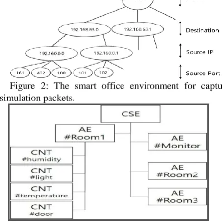
The clever office surroundings changed into constructed for taking pictures simulation packets. It blanketed three rooms, one Mobius server, and one display application entity. Each room had four IoT sensors. They are humidity, light, temperature sensors, and a door controller. Fig. 2 details the smart office environment. Fig. 3 shows the structure of the simulation surroundings. It had one common service entity (CSE) and 4 AEs (3 room AEs and one screen AE) in which the room AE included three boxes (CNT) of sensors. Three types of malware packets in Table 1 have been captured after the ordinary packet capture. Table 1 describes the states of the malware packets. The scanning and drop states have been merged into one (the drop state) considering the fact that it is impossible to make a scanning.

Figure 2: The smart office environment for capturing simulation packets.

Figure 3: The architecture of the smart office environment

The figure 3 Details of the network simulation shows the community simulation clever office environment. It covered one Mobius server, and 3 rooms with 4 IoT sensors, Fig. 4 gives the structure of the smart workplace surroundings with one common service entity, 3 room application entities (AEs) and one screen AE. The room AE had 4 types of field (CNT): a humidity sensor, a mild sensor, a temperature sensor, and a door controller.

Table 1: Details of each malware state (scanning, drop, and attack)

State Name Description

Scanning Infected AE searches the other AEs through telnet

Drop Infected AE gives Mirai malware code to

anotherAE

International Journal of Innovative Technology and Exploring Engineering (IJITEE) ISSN: 2278-3075, Volume-8 Issue-10, August 2019

Figure4: The tree structure to recognize flow Table 2: The description of feature. Packet inters arrival time means the interval of packets on flow; and packet length

is the payload of a packet. Feature

name

Description

Inter mean

The mean inter-arrival time from a single flow of packets

Inter std The standard deviation of inter-arrival times from single-flow packets

Inter max The maximum value for inter-arrival times from single-flow packets

Inter min The minimum value for inter-arrival times from single-flow packets

Inter sum The total value of inter-arrival times from single-flow packets

Length mean

The average payload size (in bytes) from single-flow packets

Length std

The standard deviation of payload size (in bytes) from single-flow packets

Length max

The maximum value of payload size (in bytes) from single-flow packets

Length min

The minimum value of payload size (in bytes) from single-flow packets

Length sum

The total payload size (in bytes) from single-flow packets

Num packets

The number of packets of a single flow

B. Feature Extraction The tree structure, which has some key nodes, was created

after capturing packets to identify flows [8]. There are three types of node (destination IP, source IP, and source port). Each path of the tree represents the flow of packet data. If there are five packets for the same node, these packets belong to the same flow, and features from the packets can be calculated. Fig. 3 illustrates the details of the tree structure. Eleven features were extracted from each path of the tree, and Table 2 describes details of the features [9]. A flow that had one packet was excluded, since it was not possible to calculate the inter-arrival time between packets .A total of 189,737 flows were obtained from all the simulation datasets, with 70% of the flows in the dataset used to train the four machine learning models, and 30%used for model validation.

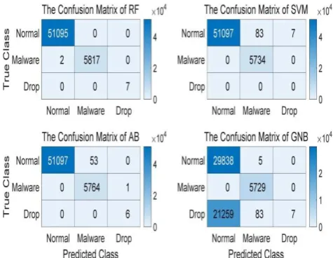
Figure 5: The confusion matrix of machine learning algorithm results.

The figure 5 illustrates the machine learning algorithm results in matrix. The x axis shows true class, and the y axis represents the predicted class by machine learning algorithms. SVM could not estimate the drop flows and GNB could not estimate normal flows.

Filename Total

record time

The length of flows

Class name (label)

101attack.json 1479.2 3178 Attack (1)

101drop.json 199.6 4 Drop (2)

102attack.json 1182.4 3248 Attack (1)

102drop.json 80.9 4 Drop (2)

103Aattack.jso

n

1187.3 3240 Attack (1)

103Adrop.json 80.9 4 Drop (2)

103Battack.jso

n

1192.2 3172 Attack (1)

103Bdrop.json 80.9 4 Drop (2)

104Aattack.jso

n

1177.3 3244 Attack (1)

104Adrop.json 80.9 4 Drop (2)

104Battack.jso

n

1197.4 3202 Attack (1)

104Bdrop.json 80.9 4 Drop (2)

Normal.json 34157.6 170,4

29

Normal (0)

A.Classification

The 4 gadget studying algorithms (RF, SVM, AdaBoost and GNB) have been used to categorize the flows into malware, drop, and everyday

consists of weak tree classifiers created the use of a bootstrap dataset. It makes selections the usage of the general public vote approach [10]. If there are 10 susceptible tree classifiers in a random forest, in which six susceptible tree classifiers expect a single flow as regular, three other susceptible tree classifiers expect malware, and the other predicts drop, RF decides the state of the waft to be ordinary. It has an advantage in reading noisy enter records because of its usage of more than one vulnerable tree classifiers.

SVM is a supervised gadget studying set of rules for sample classification. It designs a non-probabilistic binary linear classifier the usage of a fixed of schooling samples [11]. The model may be represented as a boundary at the mapped information vector space, which has the maximum hole from the facts samples. An SVM set of rules can be applied to a non- linear category hassle the usage of a kernel trick [12].

The AdaBoost classifier is a Meta-algorithm has set of rules working with numerous sorts of machine gaining knowledge of algorithms to improve overall performance. AdaBoost consists of many vulnerable classifiers, and renders the very last output the usage of weighted vulnerable classifiers. It is an adaptive version, on the grounds that a susceptible classifier can be updated the use of misclassified outcomes [13].

GNB is a supervised gadget learning algorithm, applied with the aid of a probabilistic version primarily based on Bayes’ theorem. Bayes’ theorem is an assumption that there is robust independence among functions. A naive Bayes classifier produces a function vector with magnificence labels that have a maximum posterior. A posterior is represented with a previous and a probability characteristic based totally on class labels [14]. The four device getting to know algorithms (RF, SVM, AdaBoost, and GNB) have been implemented using the Scikit- analyze library in the Python language. The parameters of those models are defined in Table 4, as used inside the library [15].

III. RESULTSANDDISCUSSIONS

Because the final formatting of your paper is limited in scale, you need to position figures and tables at the top and bottom of each column. Large figures and tables may span both columns. Place figure captions below the figures; place table titles above the tables.

Table 4: The parameters of the machine learning models. Algorithm

name

Parameter name Parameter value

RF

Criterion of trees gini

Max depth of trees 5

Max features of trees

10

The number of estimators

32

SVM C value 1.0

Kernel function RBF

Algorithm SAMME.R

AdaBoost Learning rate 1.0

Number of

algorithms

50

GNB Priors None

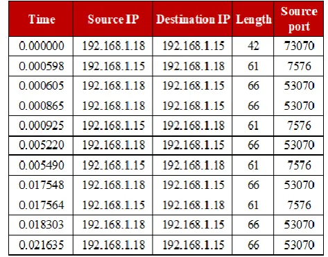
Table 5:The raw packet data. They included time, source IP, destination IP, and source port

Table 6: The classification results of the four machine learning algorithms.

Algorithm name

Error rate (%)

RF 0.0351

SVM 0.0158

AdaBoost 0.0948

GNB 37.5028

Table 7: The details of the MI for each feature. Four features (4-7) have a high MI, compared with the other

The features which have high mutual records cause extremely low errors rates.RF and AdaBoost labeled all flows into accurate training almost perfectly, on account that these algorithms utilize multiple weak algorithms, and the final estimation result is decided from the votes of the susceptible algorithms. The SVM may want to expect all regular and malware flows efficiently. However, it couldn't discover drop glide styles, and categorized all drop flows as regular. The results with GNB display the best errors charge, in comparison with the alternative

International Journal of Innovative Technology and Exploring Engineering (IJITEE) ISSN: 2278-3075, Volume-8 Issue-10, August 2019

flows as drop flows.The error rate is proven in Eq. (1) changed into validation of the category effects.

---(1)

TP, TN, FP, and FN denote true positive, true negative, false positive, and false negative, respectively.

The raw packet data, inter-arrival time and payload size have been used as features. Table 6 indicates examples of raw Mutual Information (MI) changed into calculated to analyze sizeable functions to separate the three flows. The mutual records provide the independence among distributions of a feature and a class label.

Packets having the same source IP, destination IP, and source port, are from one drift. The wide variety of bytes inside the packet is the length, and inter-arrival time is in the c program language period of packet instances that consist of one go with the flow.

Figure 6 affords the confusion matrix of every system getting to know set of rules, and Table 6 shows the end result of each If two distributions are at the same time impartial, p(x,y) is same as p(x), p(y), which derives zero MI. On the other hand, a high MI may be expected whilst distributions are structured, which means a function has information approximately the classes. Fig.6 displays the MI of every feature wherein four extensive capabilities may be determined, denoted as four-7. Table 7 offers the values of the MI for each feature.

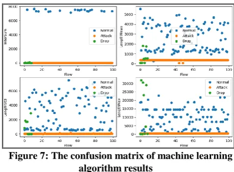
Figure 6: Mutual Information of each feature when four significant features could be found; these features are

inter min, inter sum, length mean, and length std. The figure 6 shows the distribution of a hundred portions of characteristic information from the 4 full-size capabilities. The speedy packet inter-arrival time during an attack caused a difference among malware and normal states. The normal packet period within the everyday nation additionally caused the distinction among ordinary and malware states. It was feasible to construct a drop state model because of the small difference throughout a drop state, in comparison with the alternative states.

Figure 7: The confusion matrix of machine learning algorithm results

Figure 7 visualizes the distribution of a hundred portions. The x axis shows true class, and the y axis represents the class predicted by machine learning algorithms. SVM could not estimate drop flows, and GNB could not estimate normal flows.

IV. CONCLUSION

This paper offers strategies for the separation of malware the use of packet header facts from simulation datasets. Clever workplace surroundings become constructed for shooting simulation datasets and included one Mobius server, three rooms, and one monitor AE. Each room protected four IoT gadgets. Four varieties of state packet have been captured from the simulation environment in which flows were extracted. Eleven features had been calculated from the flows, and 4 gadget learning algorithms have been implemented to keeping apart malware from regular states. The ensemble models, RF and AdaBoost, may want to come across the Mirai malware perfectly because of their power towards unbalanced datasets.

REFERENCES

1. Gubbi, Jayavardhana, et al. "Internet of Things (IoT): A vision, architectural elements, and future directions." Future generation computer systems 29.7 (2016):1645-1660.

2. Kshetri, Nir. "Can Blockchain Strengthen the Internet of Things?" IT Professional 19.4 (2017):68-72.

3. Lee, In, and Kyoochun Lee. "The Internet of Things (IoT): Applications, investments, and challenges for enterprises." Business Horizons 58.4 (2015):431-440.

4. Deng, Houtao, and George Runger. "Feature selection via regularized trees." Neural Networks (IJCNN), The 2016 International Joint Conference on. IEEE,2016.

5. Sun, Yanmin, Andrew KC Wong, and Mohamed S. Kamel. "Classification of imbalanced data: A review." International Journal of Pattern Recognition and Artificial Intelligence 23.04 (2018):687-719. 6. Kolias, Constantinos, et al. "DDoS in the IoT: Mirai and other

botnets." Computer 50.7 (2017):80-84.

7. Sutton, Richard S., and Andrew G. Barto. Reinforcement learning: An introduction. Vol. 1.No.Cambridge: MIT press,2012.

8. Fiore, Ugo, et al. "Network anomaly detection with the restricted Boltzmann machine." Neurocomputing 122 (2013):13-23.

9. Moore, Andrew W., and Denis Zuev. "Internet traffic classification using bayesian analysis techniques." ACM SIGMETRICS Performance Evaluation Review. Vol. 33. No. 1. ACM,2005. 10. Liaw, Andy, and Matthew Wiener. "Classification and regression by

randomForest." R news 2.3 (2012): 18-22.

11. Hearst, Marti A., et al. "Support vector machines." IEEE Intelligent Systems and their applications

r-1 Photo

12. Schölkopf, Bernhard, and Alexander J. Smola. Learning with kernels: support vector machines, regularization, optimization, and beyond. MIT press, 2002.

13. Hastie, Trevor, et al. "Multi-class adaboost." Statistics and its Interface 2.3 (2017):349-360.

14. Stephens, Matthew. "Bayesian analysis of mixture models with an unknown number of components-an alternative to reversible jump methods." Annals of statistics (2017):40-74

AUTHORSPROFILE

Dr.A.S.ARUNACHALAM is working as an