TITLE
Computational Sciences and Parallelism
BYLINE
Geoffrey Fox
School of Informatics and Computing And Pervasive Technology Institute Indiana University
Bloomington IN
SYNONYMS
Applications and Parallelism
Problem Architectures
DEFINITION
Here we ask which applications should run in parallel and correspondingly which areas of computational science will benefit from parallelism. In studying this we will discover which applications benefit from particular hardware and software choices. A driving principle is that in parallel programming, one must map problems into software and then into hardware. The architecture differences in source and target of these maps will affect the efficiency and ease of parallelism.
DISCUSSION
Introduction
I have an application – can and should it be parallelized and if so, how should this be done and what are appropriate target hardware architectures; what is known about clever algorithms and what are recommended software technologies? Fox introduced in [1] a general approach to this question by considering problems and the computer
infrastructure on which they are executed as complex systems. Namely each is a
collection of entities and connections between them governed by some laws. The entities can be illustrated by mesh points, particles, data points for problems; cores, networks and storage locations for hardware; objects, instructions and messages for software. The processes of deriving numerical models, generating the software to simulate model, compiling the software, generating the machine code and finally executing the program on particular hardware can be considered as maps between different complex systems. Many performances models and analyses have been developed and these describe the quality of map. We know that maps are essentially never perfect and describing
must be high. In this discussion, we want to describe the issues of parallelism and here there are two particularly interesting general results. Firstly we can usually define a space (the domain of entities) and a time associated with a complex system. Time is nature’s time for the complex system that describes time dependent simulations. However for linear algebra time for that complex system is an iteration count. Note for the simplest sequential computer hardware there is no space and just a time defined by the control flow. Thus in executing problems on computers one is typically mapping all or part of the space of the problem onto time for the computer and parallel computing corresponding case where both problem and computer have well defined spatial extent. Mapping is usually never 1:1 and reversible and “information is lost” as one maps one system into another. In particular one fundamental reason why automatic parallelism can be hard is that the mapping of problem into software has thrown away key information about the space-time structure of original problem. Language designers in this field try to find languages that preserve key information needed for parallelism while hardware designers design computers that can work around this loss of information. For an example use of arrays in many data parallel languages from APL, HPF to Sawzall, can be viewed as a way to preserve spatial structure of problems when expressed in these languages. In this article, we will not discuss these issues in depth but rather discuss what is possible with “knowledgeable users” mapping problems to computers or particular programming paradigms.
Simple Example
We consider the simple case of a problem whose complex system spatial structure is represented as a 2D mesh. This comes in material science when one considers local forces between a regular array of particles or in the finite difference approach to solving Laplace or Poisson’s equation in two dimensions. There are many important subtleties such as adaptive meshes and hierarchical multigrid methods but in the simplest
formulation such problems are set up as a regular grid of field values where the basic iterative update links nearest neighbors in two dimensions.
If the points are labeled by an index pair (i,j), then Jacobi's method (not state of the art but chosen as simplicity allows a clear discussion) can be written
φ (i,j) is replaced by (φLeft + φRight + φUp + φDown ) / 4 (1) where φLeft =φ (i,j-1)and similarly for φRight, φUp, and φDown.
Such problems would usually be parallelized by a technique that is often called "domain decomposition" or "data parallelism" although these terms are not very precise.
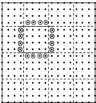
Parallelism is naturally found for such problems by dividing the domain up into parts and assigning each part to a different processors as seen in Figure 1. Here the problem
represented as a 16x16 mesh is solved on a 4x4 mesh of processors. For problems coming from nature this geometric view is intuitive as say in a weather simulation, the
distributed memory or implicitly in a shared memory) that implements this eventual mixing.
Figure 1: Communication Structure for 2D Complex System Example. The dots are the 256 points in the problem. Shown by dashed lines is the division into 16 processors. The circled
points are the halo or ghost grid points communicated to processor they surround.
Such block data decompositions typically lead to a SPMD (Single Program Multiple Data) structure with each processor executing the same code but on different data points and with differing boundary conditions. In this type of problem, processors at the edge of the (4x4) mesh do not see quite the same communication and compute complexity as the “general case” of an inside processor shown in figure 1. For the local nearest neighbor structure of Equation (1), one needs to communicate the ring of halo points shown in figure. As computation grows like the number of points (grain size) n in each processor and communication like the number on edge (proportional to √n), the time “wasted” communicating decreases as a fraction of the total as the grain size n increases. Further one can usually "block" the communication to transmit all the needed points in a few messages as latency can be an important part of communication overhead.
Note that this type of data decomposition implies the so-called “owner’s-compute” rule. Here we imagine each data point as being owned by the processor to which the
decomposition assigns it. The owner of a given data-point is then responsible for
performing the computation that “updates” its corresponding data values. This produces a common scenario where parallel program consists of a loop over iterations divided into compute-communicate phases:
• Communicate: At the start of each iteration, first communicate any outside data values needed to update the data values at points owned by this processor. • Compute: Perform update of data values with each processor operating without
need to further synchronize with other machines.
point which naturally scales. The above discussion uses a terminology natural for distributed memory hardware or message passing programming models. With a shared memory model like OpenMP, communication would be implicit and the “communication phase” above would be implemented as a barrier synchronization.
Performance Model
We can use our current Poisson equation example to illustrate some simple techniques that allow estimates of the performance of many parallel programs.
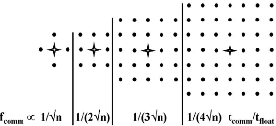
Figure 2: Parameters determining performance of loosely synchronous problems.
As shown in Figure 4.5, we characterize the node of a parallel machine by a parameter tfloat, which is time taken for a single floating point operation. tfloat is of course not very well defined as depends on the effectiveness of cache, possible use of fused multiply-add and other issues. This implies that this measure will have some application dependence reflecting the goodness of the match of the problem to the node architecture. We let n be the grain size – the number of data points owned by a typical processor. Communication performance – whether through a shared or distributed memory architecture – can be parameterized as
Time to communicate Ncommwords = tlatency + Ncommtcomm (2)
This equation ignores issues like bus or switch contention but is a reasonable model in many cases. Latencies tlatencycan be around 1 microsecond on high performance systems but is measured in millisecondsin a geographically distributed grid. tcomm is time to communicate a single word and for large enough messages, the latency term can be ignored which we will do in thefollowing.
Parallel performance is dependent on load balancing and communication and both can be discussed but here we focus on communication with problem of figure 1 generalized to Nproc processors arranged in an √Nproc by √Nproc grid with a total of N mesh points and the grain size n = N/Nproc. Let T(Nproc) be the execution time on Nproc processors and we find two contributions to this ignoring small load imbalances from edge processors. There is a calculation time expressed as n tcalcwith tcalc = 4 tfloatas the time to execute the basic update equation (1). In addition the parallel program has communication overhead, which adds to T(Nproc) a term 4√n tcomm. Now we find the speed up formula:
S(Nproc) =T(1)/ T(Nproc)= Nproc / (1 + tcomm/(√n tfloat)) (3)
We note that this analysis ignores the possibility available on some computers of overlapping communication and computation which is straightforwardly included. We can generalize the above formalism most conveniently using the notation that
which defines efficiency ε and overhead f. Note that we prefer to discuss overhead rather than speed-up or efficiency as one typically gets simpler models for f as the effects of parallelism are additive to f but for example occur in the denominator of equation (3) for speedup and efficiency. The communication part fcomm of the overhead f is given by combining equations (3) and (4) as
fcomm = tcomm/(√n tfloat) (5)
Note that in many instances, fcomm can be thought of as simply the ratio of parallel communication to parallel computation. This equation can be generalized to essentially all problems we will later term loosely synchronous. Then in each coupled communicate-compute phases of such problems, one finds that the overhead takes the form:
fcomm = constant . tcomm/(n1/d tfloat) (6)
Here d is an appropriate (complexity or information) dimension, which is equal to the geometric dimension for partial differential based equations or other geometrically local algorithms such as particle dynamics. A particularly important case in practice is the 3D value d=3 when n-1/dis just surface/volume in three dimensions. However equation (6) describes many non geometrically local problems with for example the value d=2 for the best decompositions for full matrix linear algebra and d=1 for long range interaction problems. The Fast Fourier Transform FFT finds n1/d in equation (6) replaced by ln(n) corresponding to d=∞.
From equation (4), we find that S(Nproc) increases linearly with Nproc as long as Nproc is increased with fixed fcomm which implies fixed grain size n, while tcomm and tfloat are naturally fixed. This is scaled speedup where the problem size N = nNproc also increases linearly with Nproc. The continuing success of parallel computing even on very large machines can be considered as a consequence of equations like (6) as the formula for fcomm only depends on local node parameters and not on the number of processors. Thus as we scale up the number of processors keeping the node hardware and application grain size n fixed, we will get scaling performance – speedup proportional to Nproc. Note this implies that total problem size increases proportional to Nproc – the defining characteristic of scaled speedup.
Complex Applications are better for Parallelism
The simple problem described above is perhaps the one where the parallel issues are most obvious; however it is not the one where good parallel performance is easiest to obtain as the small computational complexity of the update equation (1) makes the communication overhead relatively more important. There is a fortunate general rule that as one increases the complexity of a problem, the computation needed grows faster than the
number of links per entity and this is small (four in the 2-D mesh considered above) for this problem class.
As an illustration of the effect varying computational complexity, we see in figure 3 how the above analysis is altered as one changes the update formula of equation (1). We can now systematically increase the size of the stencil parameterized by an integer l and find how fcomm changes. In the case where points are particles the value of l corresponds to the range of their mutual force and in the case of discretization of partial differential
[image:6.612.166.448.200.329.2]equations l measures the order of the approximation.
Figure 3: Communication Structure as a function of stencil size. The figure shows 4 stencils with from left to right, range l = 1,1,2,3.
We find that the communication overhead decreases systematically as shown in Figure 3 as the range of the force increases. The general 2D result is:
fcomm ∝ tcomm/(l √n tfloat) (7)
This is valid for l which is large compared to 1 but smaller than the length scale corresponding to region stored in each processor. In the interesting limit of an infinite range ( l→∞) force, the analysis needs to be redone and one finds the result that is independent of the geometric dimension
fcomm ∝ tcomm/(n tfloat) (8)
which is of the general form of equation (6) with complexity dimension d=1. This is the best-understood case where the geometric and complexity dimensions are different. The overhead formula of equation (8) corresponds to the computationally intense O(N2) algorithms for evolving N-body problems. The amount of computation is so large that the ratio of communication to computation is extremely small.
Application Architectures
The analysis above can be applied to many SPMD problems and addresses the matching of “spatial” structure of applications and computers. This drives needed linkage of individual computers in a parallel system in terms of topology and performance of network. However this only works if we can match the temporal structure and this aspect is more qualitative and perhaps controversial. The simplest ideas here underlied the early SIMD (Single Instruction Multiple Data) machines that were popular some 20 years ago. These are suitable for problems where each point of the complex system evolves with the same rule (mapping into machine instruction) at each time. There are many such
related problems do not fit this structure – called synchronous in [1] – with the simplest reason being heterogeneity in system requiring different computational approaches at different points. A huge number of scientific problems fit a more general classification – loosely synchronous. Here we see SPMD applications which have the
compute-communication stages described above but now the compute phases are different on different processors. One uses load balancing methods to ensure that the computational work on each node is balanced but not on each machine instruction but rather in a coarse grain fashion at every iteration or time-step – whatever defines the temporal evolution of the complete system. Loosely synchronous problems fit naturally MIMD machines with the communication stages at macroscopic “time-steps” of the application. This
communication ensures the overall correct synchronization of the parallel application. Thus overhead formulae like equations (5) and (6) describe both communication and synchronization overhead. As this overhead only depends on local parameters of the application, we understand why loosely synchronously can get good scalable
performance on the largest supercomputers. Such applications need no expensive global synchronization steps. Essentially all linear algebra, particle dynamics and differential equation solvers fall in the loosely synchronous class. Note synchronous problems are still around but they are run on MIMD (Multiple Instruction Multiple Data) machines with the SPMD model.
A third class of problems – termed asynchronous -- consists of asynchronously interacting objects and is often people’s view of a typical parallel problem. It probably does describe the concurrent threads in a modern operating system and some important applications such as event driven simulations and areas like search in computer games and graph algorithms. Shared memory is natural for asynchronous problems due to low latency often needed to perform dynamic synchronization. It wasn’t clear in the past but now it appears this category is not very common in large scale parallel problems of importance. The surprise of some at the practical success of parallel computing can perhaps be understood from people thinking about asynchronous problems whereas its loosely synchronous and pleasingly parallel problems that dominate. The latter class is the simplest algorithmically with disconnected parallel components. However the
importance of this category has probably grown since the original 1988 analysis[2] when it was estimated as 20% of all parallel computing. Both Grids and clouds are very natural for this class which does not need high performance communication between different nodes. Parameter searches and many data analysis applications of independent
observations fall into this class.
From the start, we have seen a fifth class -- termed metaproblems – which refer to the coarse grain linkage of different “atomic” problems . Here synchronous, loosely synchronous, asynchronous and pleasingly parallel are the atomic classes. Metaproblems are very common and expected to grow in importance. One often uses a two level
programming model in this case with the metaproblem linkage specified by workflow and the component problems with traditional parallel languages and runtimes. Grids or Clouds are suitable for metaproblems as coarse grain decomposition does not usually require stringent performance
analysis. Nearly all the early work on parallel computing focused on simulation as opposed to data analysis (or what some call data intensive applications). Data analysis has exploded in importance recently [3] correspondingly to growth in number of instruments, sensors and human (the web) sources of data.
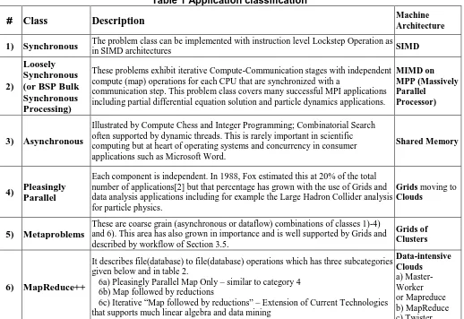
Table 1 Application classification
# Class Description Machine Architecture
1) Synchronous The problem class can be implemented with instruction level Lockstep Operation as in SIMD architectures SIMD
2)
Loosely Synchronous (or BSP Bulk Synchronous Processing)
These problems exhibit iterative Compute-Communication stages with independent compute (map) operations for each CPU that are synchronized with a
communication step. This problem class covers many successful MPI applications including partial differential equation solution and particle dynamics applications.
MIMD on MPP (Massively Parallel
Processor)
3) Asynchronous
Illustrated by Compute Chess and Integer Programming; Combinatorial Search often supported by dynamic threads. This is rarely important in scientific computing but at heart of operating systems and concurrency in consumer applications such as Microsoft Word.
Shared Memory
4) Pleasingly Parallel
Each component is independent. In 1988, Fox estimated this at 20% of the total number of applications[2] but that percentage has grown with the use of Grids and data analysis applications including for example the Large Hadron Collider analysis for particle physics.
Grids moving to Clouds
5) Metaproblems
These are coarse grain (asynchronous or dataflow) combinations of classes 1)-4) and 6). This area has also grown in importance and is well supported by Grids and described by workflow of Section 3.5.
Grids of Clusters
6) MapReduce++
It describes file(database) to file(database) operations which has three subcategories given below and in table 2.
6a) Pleasingly Parallel Map Only – similar to category 4 6b) Map followed by reductions
6c) Iterative “Map followed by reductions” – Extension of Current Technologies that supports much linear algebra and data mining
Data-intensive Clouds a) Master-Worker or Mapreduce b) MapReduce c) Twister
The MapReduce++ category has three subdivisions a) “map only” applications similar to pleasingly parallel category; b) The classic MapReduce with file to file operations consisting of parallel maps followed by parallel reduce operations.; c) captures the extended MapReduce introduced in [4-10]. Note this category has the same complex system structure as loosely synchronous or pleasingly parallel problems but is distinguished by the reading and writing of data. This comparison is made clearer in Table 2. Note nearly all early work on parallel computing discussed computing with data on memory. MapReduce and languages like Sawzall [11] and Pig-Latin [12] emphasize the parallel processing of data on disks -- a field that until recently was only covered by database community.
• Document conversion (e.g. PDF->HTML)
• Brute force
searches in cryptography
• Parametric sweeps • Gene assembly
• Much data
analysis of independent
samples
• High Energy Physics (HEP) Histograms • Distributed
search
• Distributed sort • Information
retrieval • Calculation of
Pairwise Distances for sequences (BLAST)
• Expectation maximization algorithms • Linear Algebra • Datamining including • Clustering
• K-means
• Multidimensional Scaling (MDS)
• Many MPI
scientific applications utilizing wide variety of communication constructs including local interactions • Solving differential
equations and
• Particle dynamics with short range forces
Domain of MapReduce and Iterative Extensions MPI
Summary
Problems are set up as computational or numerical systems and these can be considered as a “space” of linked entities evolving in time. We have discussed the spatial structure (which is critical for performance) and the temporal structure which is critical to
understand the class of software and computer needed. These we termed "basic complex systems" and characterized them by their possibly dynamic spatial (geometric) and temporal structure. We have noted the difference between the structure of the original problem and that of computational system derived from it. We can summarize much of the past experience in parallelizing applications by the conclusion:
Synchronous and Loosely Synchronous problems perform well on large parallel
machines as long as the problem is large enough. For a given machine, there is a typical sub-domain size (i.e. the grain size or size of that part of the problem stored on each node) above which one can expect to get good performance. There will be a roughly constant ratio of parallel speedup to Nproc if one scales the problem with fixed sub-domain size and total size proportional to Nproc. This conclusion has been enriched by study of grids and clouds with an emphasize on pleasingly parallel and MapReduce++ style problems often with a data intensive focus. These also parallelize well.
BIBLIOGRAPHIC NOTES AND FURTHER READING
Amdahl’s law[17]. The recent spate of papers on MapReduce [4, 7] and its applications and extensions[4-12, 15] allow one to extend the discussion of parallelism from
simulation (which implicitly dominated the early work) to data analysis[3].
BIBLIOGRAPHY
1. Fox, G.C., R.D. Williams, and P.C. Messina, Parallel computing works! 1994: Morgan Kaufmann Publishers, Inc.
http://www.old-npac.org/copywrite/pcw/node278.html#SECTION001440000000000000000
2. Fox, G.C., What Have We Learnt from Using Real Parallel Machines to Solve Real Problems, in Third Conference on Hypercube Concurrent Computers and Applications, G.C. Fox, Editor., 1988, ACM Press: Vol. 2. pages. 897-955. 3. Jim Gray, Tony Hey, Stewart Tansley, and Kristin Tolle. The Fourth Paradigm:
Data-Intensive Scientific Discovery. 2010 [accessed 2010 October 21]; Available from:
http://research.microsoft.com/en-us/collaboration/fourthparadigm/.
4. J.Ekanayake, H.Li, B.Zhang, T.Gunarathne, S.Bae, J.Qiu, and G.Fox, Twister: A Runtime for iterative MapReduce, in Proceedings of the First International Workshop on MapReduce and its Applications of ACM HPDC 2010 conference June 20-25, 2010. 2010, ACM. Chicago, Illinois.
http://grids.ucs.indiana.edu/ptliupages/publications/hpdc-camera-ready-submission.pdf.
5. Yingyi Bu, Bill Howe, Magdalena Balazinska, and Michael D. Ernst, HaLoop: Efficient Iterative Data Processing on Large Clusters, in The 36th International Conference on Very Large Data Bases. September 13-17, 2010, VLDB
Endowment: Vol. 3. Singapore.
http://www.ics.uci.edu/~yingyib/papers/HaLoop_camera_ready.pdf. 6. Bingjing Zhang, Yang Ruan, Tak-Lon Wu, Judy Qiu, Adam Hughes, and
Geoffrey Fox, Applying Twister to Scientific Applications, in CloudCom 2010. November 30-December 3, 2010. IUPUI Conference Center Indianapolis.
http://grids.ucs.indiana.edu/ptliupages/publications/PID1510523.pdf. 7. Dean, J. and S. Ghemawat, MapReduce: simplified data processing on large
clusters. Commun. ACM, 2008. 51(1): p. 107-113.
8. Jaliya Ekanayake,Ph. D. Thesis ARCHITECTURE AND PERFORMANCE OF RUNTIME ENVIRONMENTS FOR DATA INTENSIVE SCALABLE
COMPUTING, in School of Informatics and Computing. December, 2010, Indiana University: Bloomington.
http://grids.ucs.indiana.edu/ptliupages/publications/thesis_jaliya_v24.pdf
9. Grzegorz Malewicz, Matthew H. Austern, Aart J. C. Bik, James C. Dehnert, Ilan Horn, Naty Leiser, and Grzegorz Czajkowski, Pregel: A System for Large-Scale Graph Processing, in International conference on Management of data. 2010. Indianapolis, Indiana, USA. pages. 135-146.
on Hot Topics in Cloud Computing (HotCloud '10). June 22, 2010. Boston.
http://www.cs.berkeley.edu/~franklin/Papers/hotcloud.pdf.
11. Pike, R., S. Dorward, R. Griesemer, and S. Quinlan, Interpreting the data: Parallel analysis with sawzall. Scientific Programming Journal Special Issue on Grids and Worldwide Computing Programming Models and Infrastructure, 2005. 13(4): p. 227–298. http://iospress.metapress.com/content/99VJKGKAE3JKVU9T
12. Christopher Olston, Benjamin Reed, Utkarsh Srivastava, Ravi Kumar, and Andrew Tomkins, Pig latin: a not-so-foreign language for data processing, in Proceedings of the 2008 ACM SIGMOD international conference on
Management of data. 2008, ACM. Vancouver, Canada. pages. 1099-1110.
http://portal.acm.org/citation.cfm?id=1376726.
13. Jack Dongarra, Ian Foster, Geoffrey Fox, William Gropp, Ken Kennedy, Linda Torczon, and Andy White, The Sourcebook of Parallel Computing. 2002: Morgan Kaufmann. ISBN:978-1558608719
14. Fox, G.C. and P. Coddington, Parallel computers and complex systems, in Complex Systems: From Biology to Computation, T.R.J. Bossomaier and D.G. Green, Editors. 2000, Cambridge University Press. p. 272-287.
http://cs.adelaide.edu.au/~paulc/papers/sccs-370b/abs-0370b.html.
15. Jaliya Ekanayake, Thilina Gunarathne, Judy Qiu, Geoffrey Fox, Scott Beason, Jong Youl Choi, Yang Ruan, Seung-Hee Bae, and Hui Li, Applicability of DryadLINQ to Scientific Applications. January 30, 2010, Community Grids Laboratory, Indiana University.
http://grids.ucs.indiana.edu/ptliupages/publications/DryadReport.pdf.
16. Gustafson, J.L., Reevaluating Amdahl's law. Commun. ACM, 1988. 31(5): p. 532-533. DOI:10.1145/42411.42415
17. Wikipedia. Amdahl's law. [accessed 2010 December 28]; Available from: