Detailed Results of Evaluation of DAVS(c) Deterministic Annealing Clustering and its Application to LC MS Data Analysis

(1)

Detailed Results of Evaluation of DAVS(c) Deterministic Annealing

Clustering and its Application to LC-MS Data Analysis

Geoffrey Fox (gcf@indiana.edu) D. R. Mani (manidr@broad.mit.edu) Saumyadipta Pyne (spyne@broadinstitute.org)

Abstract

We present a scalable parallel deterministic annealing formalism for clustering with cutoffs and position dependent variances. We apply it to “peak matching" problem of identifying the common LC-MS peaks across multiple samples in proteomic biomarker discovery.

1 Introduction

This paper extends the deterministic annealing approach of [1] to a scalable integrated parallel formulation. It extends earlier work [2-4] to add cutoff clusters and parallelism. It also addresses special features of the LC-MS problem including the very different scales in the m/z and RT dimensions. The large number of clusters (around 30,000 for a quarter of a million peaks) also requires new approaches to the parallel approach discussed in [5-9] top get efficient scalable performance. Also note most of the previous parallel work was not focused on vector space problems but rather on non-metric spaces[10] extending methods introduced by Hofmann and Buhmann [11] and at most around 100 clusters.

2 Parallel Deterministic Annealing Clustering with Cutoff

Deterministic annealing [4] is motivated by the same key concept as the more familiar simulated annealing method for optimization problems. At high temperatures systems equilibrate easily as there is no roughness in the energy (objective) function. If one lowers the temperature on an equilibrated system, then it is a short well-determined path between minima at current temperature and that at previous temperature. Thus systems which are equilibrated iteratively at gradually lowered temperature, tend to avoid local minima. The Monte Carlo approach of simulated annealing is often too slow, and so in deterministic annealing integrals are performed analytically. In many examples as in example here T is essentially a distance resolution; at large temperatures all clusters are merged together and they emerge as one looks at the system with sharper resolution as temperature decreases.

Consider a Hamiltonian H(χ, ϕ) which is to be minimized with respect to variables χ and ϕ. Then deterministic annealing is based on averaging with the Gibbs distribution at Temperature T.

P(χ, ϕ) = exp( - H(χ, ϕ) / T) / ∫ dχ exp( - H(χ, ϕ) / T) (1)

and one minimizes the Free Energy F combining Objective Function H and Entropy,

F = < H - T S(P) > = ∫ dχ [P(χ)H + T P(χ) lnP(χ)] (2)

One obtains an EM (Expectation Maximization) method with the variable set χ subject to annealing and determined by

χ = <χ> |0 = ∫ dχχ P(χ) (3)

And this is followed by the M step which determines the remaining parameters ϕ optimized by traditional methods. Note one iterates over temperature decreasing it gradually, but also iterates at fixed temperature until the EM step converges.

Consider a clustering problem with N points (peaks in LC-MS application) labeled by x with position X(x) and K clusters labeled by k. Let clusters have standard deviation σ(k) and center Y(k). The annealed

(2)

variables χ are Mx(k), which are the probabilities that the point x belongs to cluster k with constraint for

each point x.

∑k=1K Mx(k) = 1 (4)

Let ρ(z,σ) = 0.5 ∑i=1d (zi/σi)2 (5)

with vector dimension d for X(x) and Y(k) with d = 2 in example given later.

Define the clustering Hamiltonian

H = ∑k=0K∑x=1N Mx(k) f(x,k) (6)

With for k >= 1 f(x,k) = ρ( X(x) - Y(k), σi(k)) (7a)

and for k=0 f(x,0) = 0.5 c2_{independent of}_x_. _(7b)

Then as | X(x) - Y(k)| increases, f(x,k) becomes larger than f(x,0) which we term the sponge as it absorbs all points outside all clusters (X(x) - Y(k) / σ(k)2_{> c}2_{for all}_k_{> 0. Note there is only one sponge} but multiple conventional clusters. An important innovation introduced by Rose [4] is the use of an intrinsic probability p(k) for each cluster k satisfying

∑k=0K p(k) = 1 (8)

One can understand this as corresponding to a large number Λ (much larger than current number of centers K) of clusters with a fraction p(k) of them at each center. This allows one to split centers cleanly as one takes the number p(k) Λ at a center position and divide in two when cluster with this center splits. Without this approach, splitting is inelegant as the formalism naturally gives half a cluster at each center. The p(k) are given below and are viewed as one of variables ϕ determined at the M step of EM method. In this case, the Free Energy F is given by

F = - T ∑x=1N ln ∑k=0K p(k) exp( - f(x, k) /T ) (9)

Now we use equation (3) to determine the annealed variables < Mx(k)> and in this case, the integrals can

be done exactly as Hamiltonian is a quadratic. We describe how to tackle the case with more complicated forms for H and intractable integrals elsewhere [7, 10]. This is followed by an M step with a simple minimization to find the ϕ variables Y(k) and p(k) subject to equation (8). We introduce auxiliary variables Zxgiven by

Zx = ∑k=1K p(k) exp( - (X(x) - Y(k))2/(2 σ(k)2 T) ) + p(0)exp( - c2/(2 T)) (10)

< Mx(0)> = p(0) exp( - c2/(2 T) ) / Zx (11a)

< Mx(k)> = p(k) exp( - (X(x) - Y(k))2 / (2 σ(k)2 T) ) / Zx for k > 0 (11b)

Y(k) = ∑x=1N < Mx(k)> X(x) / ∑x=1N < Mx(k)> k≠0 (12)

p(k) = ∑x=1N <Mx(k)> / N (13)

Note in the conventional formalism p(k) = 1, small clusters contribute similarly to a big cluster in Zx

which appears in denominators like equation (11b). In equation (13), the cluster probability p(k) is the fraction of points in the k’th cluster and this implies that in (10), clusters are weighted according to their size which is intuitively attractive. The sponge k=0 is rather different from the other clusters as it will not be split and will dominate equation (8) in the case of very many individually small clusters k if we use (13) for it. So we modified (13) with a fixed p(0) that we did not vary at M step.

(3)

As explained in detail in earlier papers [4, 10], the minimized free energy (9) will exhibit instabilities corresponding mathematically to second derivatives that have negative eigenvalues. These are phase transitions in a physics terminology [3]. One can calculate the second derivatives of F

∂2_F/∂_Y

i(λ) ∂Yj(µ) = δij δµλ∑x=1N < Mx(λ)> / σi(λ)2 (14a)

- δµλ∑x=1N (Yi(λ)) - Xi(x)) (Yj(µ)) – Xj(x)) < Mx(λ)>/ (Tσi(λ)2σj(µ)2) (14b)

+ ∑x=1N (Yi(λ)) - Xi(x)) (Yj(µ)) – Xj(x)) < Mx(λ)>< Mx(µ)>/ (Tσi(λ)2σj(µ)2) (14c)

Interestingly the formula is independent of p(k) and sponge term as long as we express in terms of fractional probabilities < Mx(k)>. Equation (14) has a reasonable structure with (14b) increasing in

importance as T decreases. One examines (14) for instabilities separately for each cluster λ = µ running from 1 .. K. It is easy to see that elongated clusters will have large values of the term (14b) and these will naturally split first as T decreases. Note as T decreases the exponential in terms like (10) and (11) can lead to arithmetic errors. This was avoided by both testing on exponent and checking for overflow.

The equations above are solved by starting with one cluster at large T∞ which is determined from (14) to be so large that it is above the phase transition temperatures. The precise value is not important as the computation runs so fast with one cluster that this stage of the computation takes negligible time. Then the temperature is reduced by a factor fannealing with the EM steps above converged at each temperature. Splitting is checked at each new temperature for each cluster. If (14) is singular for cluster λ then this cluster is split and given a perturbed position determined by direction of the unstable eigenvector of ∂2_F/∂_Y

i(λ) ∂Yj(λ) and a magnitude determined so that cluster count ∑x=1N <Mx(k)> will change by a

modest amount (~5%) for each of two child clusters. This process is continued until reasonable termination criteria met. In this problem clusters were not split if their average width was small and if they were small (these cuts were set differently depending on value of cutoff c). Also clusters were removed if they were too small or if their centers were too close. As seen in figure 6, this close cluster check was only used at low temperatures i.e. at a distance scale when clusters were resolved. Clusters are considered final when the freezing factor FF given in (15) is small. Note at convergence <Mx(k)> are

either 1 or zero whereas at any “non-zero” temperature the <Mx(k)> sum to 1 for each k and are

interpreted as probabilities that are resolved at low temperature. All clusterings are finished with a set of annealing iterations where there is no splitting but one just waits that all clusters have FF < 0.002 (most are much smaller than this). The final temperature for this is around T ~ 0.01.

FF(k) = ∑x=1N <Mx(k)> ( 1 - <Mx(k)> ) / N (15)

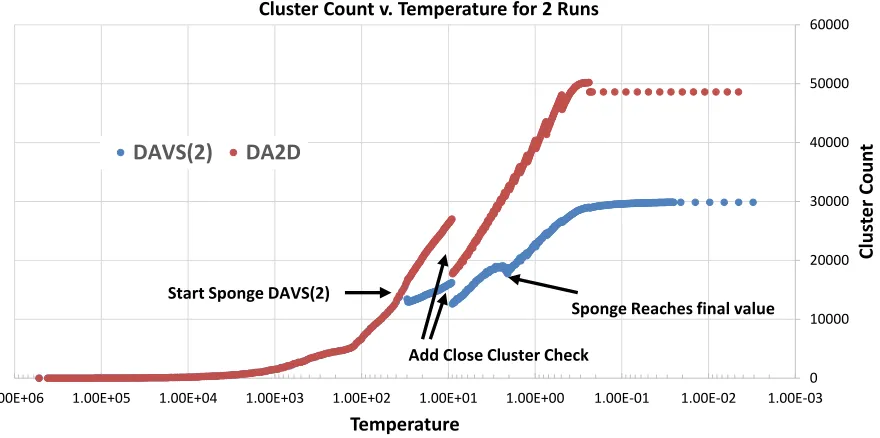
The scale represented by sponge cutoff c is much smaller than initial temperature T∞ and so we started the clustering with no sponge factor and then introduce it a lower temperature and in fact anneal it to reach its final value at low temperature. In example given later in figure 6, the desired sponge cutoff of 2 was reached at T = 2 after being introduced as a cutoff of 45 at T = 30.

In the LC-MS problem, the variance in m/z is much smaller than that of RT and if used directly would lead to anomalies as formalism designed for circular clusters. So we adjusted above formalism to make the variance in m/z anneal from a large value at T∞ to the desired value at T = 12. Note that for LC-MS the variances are the “real values” and so temperature has a natural scale with T=1 as natural “tipping point”.

The most straightforward parallelism is that of points and is implemented [10] by uniformly dividing the points between compute units (processes or threads) when the equations above consist of parallel

(4)

arithmetic and global reductions that can be implemented by either MPI or iterative MapReduce [6, 12-14]. This approach works well for initial values of temperature up to around 512 clusters. However as temperatures decrease the <Mx(k)> change character and each point becomes associated with a few

clusters (an average of 8 out of ~25000 in example below). Thus calculating terms like ∑x=1N <Mx(k)> as

a sum over all clusters becomes inefficient and an unnecessary memory use. Rather one uses a data structure that only keeps the <Mx(k)> for clusters whose centers are near each point. Further one can

exploit parallelism over clusters and both calculate and split clusters separately for the above equations in different regions. This leads to a familiar “local geometric” structure with points divided so nearby points are in the same process and local communications are used for point/clusters which are near the boundary between geometric domains. In LC-MS case, this geometric structure was implemented in one dimension with m/z splits. One finds a difficulty as a given decomposition may not be best for both point and cluster parallelism; this is well known for example in particle in the cell computations in scientific simulations. In our current results we implement the cluster parallelism for the MPI processes but not the thread parallelism. We kept the decomposition with equal number of points in each process; this led to about a factor of two load imbalance in number of clusters. We can improve this but current approach gives satisfactory performance for current LC-MS problems.

In the LC-MS problem, we repeated the steps above 2 or 3 times to get presented results. After first step, we took the peaks assigned to “sponge cluster” (k =0) and identified clusters in it that had been

incorrectly split in first step. The new clusters were merged with those from first step by annealing the combined sample starting not at T∞ but rather a low temperature T ~ 0.2. This was done at most 2 times in results presented here.

(5)

3 Results

3.1 Clustering Methods

This evaluation section includes several clustering methods. There are DAVS(c) which are the parallel multi-cluster deterministic annealing introduced in this paper with cutoff c so that all clusters are trimmed with all peaks satisfying ∆2D(x) ≤ c2 where

∆2D(x) = ((m/z|cluster center – m/z|x )/ δ(m/z))2 + ((RT|cluster center – RT|x )/ δ(RT))2 (16)

We present results for c = 1, 2 and 3 although latter case does not appear in all analyses as we consider c=3 as so large that many “incorrect” peaks are assigned to clusters. This extends Medea, which is the trimmed deterministic annealing algorithm described in [1] where deterministic annealing is applied separately to each trimmed cluster.

DA2D is the identical parallel multi-cluster deterministic annealing algorithm run without any trimming. It is a modern implementation of the algorithm introduced in [2-4].

Mclust is a model-based clustering algorithm [15] whose use for this problem is described in [1].

Landmark is sometimes used. It is a collection of reference peaks used to calibrate and evaluate methods

3.2 Computers Used

We used two Indiana University Clusters Madrid and Tempest specified below. These are running Windows HPC Server with parallelism from MPI (using MPI.Net [16] on top of Microsoft MPI) and TPL [17] for thread parallelism. All codes were written in C#. The results should be similar on Linux with Java or C++ coding.

Tempest: 32 nodes, each 4 Intel Xeon E7450 CPUs at 2.40GHz with 6 cores, totaling 24 cores per node; 48 GB node memory and 20Gbps Infiniband network connection

Madrid: 8 nodes, each 4 AMD Opteron 8356 at 2.30GHz with 4 cores, totaling 16 cores per node; 16GB node memory and 1Gbps Ethernet network connection

3.3 Structure of Data

Figure 1. The DA2D clustering at high temperature with 60 clusters determined from a run from 241605 peak charge 2 data where D(m/Z) was fixed at 0.005 and D(RT) was correctly 2.35. Each of those 60 clusters will eventually be broken into 500 smaller clusters and spread out along x axis as D(m/Z) is annealed to its final much smaller value. The sponge was not used in this run as it is only introduced at lower temperatures

(6)

[image:6.612.60.535.90.388.2]

.

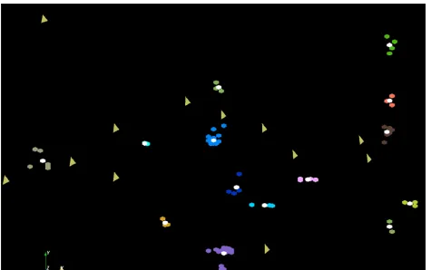
Figure 2. A tiny fragment of clustered space for a full DAVS(1) run. The orange triangles are sponge peaks outside any cluster. The colored hexagons are peaks inside clusters with the white hexagons being determined cluster centers. Each cluster is colored differently. This comes from 241605 peak charge 2 clustering.

The first two plots illustrate the nature of the data to be clustered. As the error in m/z is proportional to the inverse of this quantity, we define new 2D positions (x, y) rather than (m/z, RT)

x = ln(m/z) / D(m/Z) y = RT / D(RT)

where previous analysis of the measurement of known peaks gave D(m/Z) = 5.98 10-6_{and D(RT) = 2.35} where δ(m/z) = D(m/Z) . (m/z) and δ(RT) = D(RT) are three times standard deviation of measurement determined by study of landmark peaks. By using x and y as defined above, we get reduced variables which should give circular clusters with same size in each dimension. Note this change of variables is only used for display purposes. As described we directly use m/z and RT as coordinates in the clustering and account for position dependent error by calculating the value of δ(m/z) (and the fixed δ(RT)) dynamically for each cluster center position. The much smaller value of D(m/Z) compared to D(RT), makes the reduced space very much larger in x than y direction. This would distort the clustering algorithm at large temperatures. Thus as described, we anneal the value of D(m/Z) starting at “infinite” temperature with a large value.

(7)

[image:7.612.113.411.99.334.2]

3.4 Parallelism

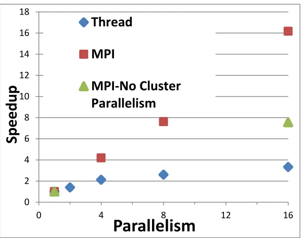
Figure 3: Parallelism within a Single Node of Madrid Cluster. A set of runs on 241605 peak data with a single node with 16 cores with either threads or MPI giving parallelism. Parallelism is either number threads or number of MPI processes. For MPI, we show case of cluster and no cluster porallelism

Figure 4: Speedups for several runs on Madrid from sequential through 128 way parallelism defined as product of number of threads per process and number of MPI processes. We look at different choices for MPI processes which are either inside nodes or on separate nodes. For example 16-way parallelism shows 3 choices with thread count 1:16 processes on one node (the fastest), 2 processes on 8 nodes and 8 processes on 2 nodes.

0 2 4 6 8 10 12 14 16 18

0 4 8 12 16

Spe

edup

Parallelism

Thread

MPI

MPI-No Cluster

Parallelism

0 10 20 30 40

0 8 16 24 32 40 48 56 64 72 80 88 96 104 112 120 128

Spe

edup

Parallelism

Speed up v Parallelism DAVS(3)

Threads 1

Threads 2

Threads 4

Threads 8

Threads 16

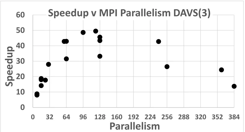
[image:7.612.73.487.388.585.2]

(8)

[image:8.612.79.474.57.270.2]

Figure 5: Speedups for several runs on Tempest from 8-way through 384 way MPI parallelism with one thread per process. We look at different choices for MPI processes which are either inside nodes or on separate nodes. Figure 3 illustrates two aspects of parallel performance. Firstly that MPI parallelism outperforms that coming from threads (compare green and blue). Secondly that we get higher performance (compare red and green) when we use the cluster parallelism described in section 2. Figure 3 only looks at parallelism within a single 16 core node whereas figures 4 and 5 extends this to up to 32 nodes where the network overheads impact performance on the runs with larger parallelism. This is especially true on the Madrid cluster which only has Ethernet network links whereas Tempest has Infiniband. Again we find MPI outperforms threading but as described earlier, we only implemented the cluster parallelism (used in all runs in this figure) with MPI. Several of these runs use a mix of thread and MPI parallelism; threads implement peak parallelism and MPI peak and cluster parallelism. All runs in figure 3 to 5 used the efficient model where each peak x only stores the occupation probability Mx(k) for relevant (i.e. nearby)

clusters k. Throughout the run (from 1 to around 25200 clusters in figures), the mean number of clusters stored for each peak averaged at most 8 which is < 0.1% of average number of clusters. Figure 3 to 5 corresponds to DAVS(3) runs.

Note that the parallel clustering is

a) Inefficient in that it is not load balanced. We currently decompose problem so there are equal number of peaks in each process. This leads to a factor of 2-4 variation in number of clusters per node. For example the case with 32 MPI processes in figure 4 finishes with an average of 789 clusters per node while the minimum number is 511and the maximum 1391.

b) Efficient as it naturally spreads splitting over the full region of peaks and this implies that cases with just one MPI process (and any number of threads) need slower annealing to get same number of clusters as runs with more than 4 MPI processes.

The parallel performance is currently limited by the load imbalance effect (a) and MPI communication overheads such that 64 way parallelism is good choice for this 241605 peak dataset on Madrid and 120 way (30 Tempest nodes with 4 MPI processes in each node) gives best speedup on Tempest. There is also the usual effects that memory bandwidth limits the useful parallelism on each node. We intend tests on larger datasets where higher levels of parallelism will be optimal. The “production” execution time used in runs reported here vary from 2 to 10 hours (dependent on annealing schedule) on the 8 node Madrid cluster which has rather old (2008) AMD processors. Tempest is a factor 1.8 faster.

3.5 Characteristics of Clustering Solutions

We present in table 1, some summary statistics over the clusterings considered here. The methods considered here are:

0

10

20

30

40

50

60

0 32 64 96 128 160 192 224 256 288 320 352 384

Spe

edup

Parallelism

Speedup v MPI Parallelism DAVS(3)

(9)

[image:9.612.73.535.69.214.2]

Table 1: Basic Statistics

Charge Method Number Clusters

Number of Clusters with occupation count

Count > 1 Scaled Error

Count > 30 Scaled Error

1 2 >2 >30 m/z RT m/z RT

2 DAVS(1) 73238 42815 10677 19746 1111 0.081 0.084 0.036 0.056 2 DAVS(2) 54055 19449 10824 23781 1257 0.191 0.205 0.079 0.100 2 DAVS(3) 41929 13708 7163 21058 1597 0.404 0.355 0.247 0.290 2 DA2D 48605 13030 9563 22545 1254 6.02 3.68 0.100 0.120 2 Mclust 84219 50689 14293 19237 917 0.048 0.060 0.021 0.041 Note that we list errors which are just the mean squared scaled differences between peaks and cluster centers.

Error(m/z) = ((m/z|cluster center – m/z|x )/ δ(m/z))2 averaged over peaks x in cluster

Error(RT) = ((RT|cluster center – RT|x )/ δ(RT))2 averaged over peaks x in cluster

The calculation in this fashion is not very reliable if clusters are not trimmed. One can calculate a much more reliable mean (as used later in comparison with Landmark clusters) by a cut like ∆2D(x) ≤ 1.2 to remove outliers.

Note both DAVS(c) and DA2D start with one cluster and then split automatically as temperature is reduced. This is illustrated earlier in figure 1 showing a high temperature with 60 clusters. Figure 6 shows how the number of clusters changes with temperature

Figure 6: Variation of cluster count in DAVS(2) and DA2D as a function of the annealing temperature as it is reduced from left to right. Changes in strategy give glitches with discontinuity in cluster count. Particularly blatant is a crude switching on of a check on closeness of cluster centers. The addition of the Sponge (trimming) factor has less impact as that effect is itself annealed as described in formalism.

0 10000 20000 30000 40000 50000 60000

1.00E-03 1.00E-02

1.00E-01 1.00E+00

1.00E+01 1.00E+02

1.00E+03 1.00E+04

1.00E+05 1.00E+06

Cl

us

te

r Co

un

t

Temperature

Cluster Count v. Temperature for 2 Runs

DAVS(2) DA2D

Start Sponge DAVS(2)

Add Close Cluster Check

Sponge Reaches final value

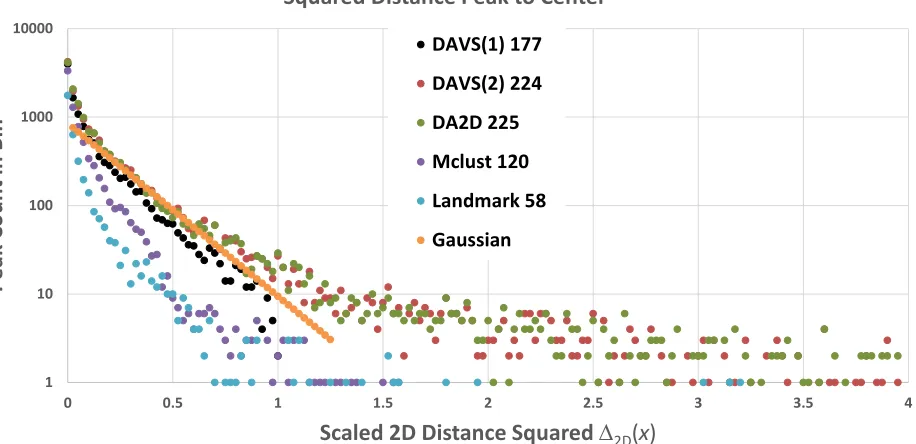
[image:9.612.87.527.353.572.2]

(10)

[image:10.612.93.542.77.342.2]

Figure 7. Histograms of ∆2D(x) for 4 different clusters methods, and the landmark set plus expectation for a

Gaussian distribution with standard deviations given as 1/3 in the two directions. The “Landmark” distribution correspond to previously identified peaks used as a control set. Note DAVS(1) and DAVS(2) have sharp cut offs at ∆2D(x) = 1 and 4 respectively. Only clusters with more than 5 peaks are plotted.

Figure 8. Histograms of ∆2D(x) for 4 different clusters methods, and the landmark set plus expectation for a

Gaussian distribution with standard deviations given as δ(m/z)/3 and δ(RT)/3 in two directions. The “Landmark” distribution correspond to previously identified peaks used as a control set. Note DAVS(1) and DAVS(2) have sharp cut offs at ∆2D(x) = 1 and 4 respectively. Only clusters with more than 50 members are plotted.

1 10 100 1000 10000

0 0.5 1 1.5 2 2.5 3 3.5 4

Pe

ak

Co

un

t i

n

Bi

n

Scaled 2D Distance Squared ∆_2D(x)

4 Clustering Methods: Occupation Count > 50 Peaks Squared Distance Peak to Center

DAVS(1) 177 DAVS(2) 224 DA2D 225 Mclust 120 Landmark 58 Gaussian

1 10 100 1000 10000 100000

0 0.5 1 1.5 2 2.5 3 3.5 4 4.5 5

Pe

ak

Co

un

t i

n

Bi

n

Scaled 2D Distance Squared

∆

_2D

(

x

)

4 Clustering Methods: Occupation Count > 5 Peaks

Squared Distance Peak to Center

DAVS(1) 8664

DAVS(2) 8755

DA2D 8749

Mclust 8194

Landmark 996

Gaussian

Method Name Followed by # Clusters

[image:10.612.82.540.424.646.2]

(11)

The next set of figures describe the characteristics of the different solutions. Figures 7 and 8 plots the squared distance distributions scaled by δ(m/z) for m/z and δ(RT) for RT in two dimensions i.e. the ordinate is ∆2D(x). These include the expectation of a Gaussian distribution in ∆2D(x) with standard deviation of 1/3 in both m/z and RT. It is normalized at ∆2D(x) ~ 0.5 to the DAVS distributions that are similar in value there.

[image:11.612.73.541.246.577.2]

We note that the four deterministic annealing solutions are quite similar at small values of ∆2D(x) ≤ 1and in each case we see a peak above the Gaussian for ∆2D(x) ≤ 0.1. Note the parallel DAVS(1) does precisely enforce the cut ∆2D(x) ≤ 1. Mclust has sharper distributions but as is made clearer with later data, it misses several clusters and many peaks that are properly associated with a given cluster.

Figure 9 shows a histogram of occupation counts for the clustering methods. Mclust tends to lie below the deterministic annealing solutions for the larger clusters.

Figure 9. Histograms of number of peaks in clusters for 4 clustering methods and the landmark set. Note lowest bin is clusters with one member peak, i.e. unclustered singletons. For DAVS these are Sponge peaks.

[image:11.612.74.539.638.721.2]

3.6 Quality of Determination of Landmark Peaks

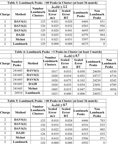
Table 2: Landmark Peaks >3 Peaks in Cluster (at least 3 match)

Total Clusters

(Not Singleton)

Singleton Cluster (Sponge)

Number Landmark

Clusters

∆2D(x) ≤ 1.2

Charge Number

Peaks Method

Scaled Error m/z

Scaled Error RT

Landmark Peaks

Non Landmark

Peaks

2 241605 DAVS(1) 30424 42815 1025 0.039 0.059 24825 6779

1 10 100 1000 10000 100000

0 20 40 60 80 100 120 140

#Cl

us

te

rs

w

ith O

cc

upa

tio

n Co

un

t

Occupation Count (Peaks in Cluster)

DAVS(1)

DAVS(2)

DA2D

Mclust

Golden

(12)

2 241605 DAVS(2) 34606 19449 1033 0.044 0.066 25012 7641 2 241605 DAVS(3) 28221 13708 1038 0.085 0.112 24939 9825 2 241605 DA2D 35472 13134 1033 0.044 0.067 24996 7606 2 241605 Mclust 33530 50948 1007 0.035 0.051 23432 4945

[image:12.612.72.483.171.670.2]

2 26916 Landmark 1263 228 1034 0.000 0.000 25151 0

Clusters

∆2D(x) ≤ 1.2

Charge Method

Scaled Error m/z Scaled Error RT Landmark Peaks Non Landmark Peaks

2 DAVS(1) 125 0.021 0.028 6468 831

2 DAVS(2) 126 0.025 0.032 6563 956

2 DAVS(3) 129 0.028 0.041 6695 1093

2 DA2D 126 0.025 0.032 6579 964

2 Mclust 111 0.021 0.031 5597 584

2 Landmark 129 0.000 0.000 6675 0

Clusters

∆2D(x) ≤ 0.7

Charge Number

Peaks Method

2 241605 DAVS(1) ₁₀₁₇ _0.033 _0.050 ₂₄₆₅₀ ₆₃₃₀

2 241605 DAVS(2) ₁₀₂₀ _0.034 _0.052 ₂₄₇₁₇ ₆₇₁₆

2 241605 DAVS(3) ₁₀₂₀ _0.075 _0.103 ₂₄₂₃₉ ₈₂₄₂

2 241605 DA2D ₁₀₂₀ _0.035 _0.054 ₂₃₆₉₁ ₆₇₀₉

2 241605 Mclust ₁₀₀₅ _0.033 _0.047 ₂₃₃₉₄ ₄₈₅₆

2 26916 Landmark ₁₀₂₃ _0.000 _0.000 ₂₄₈₅₅ ₀

Clusters

∆2D(x) ≤ 0.7

Charge Method

2 DAVS(1) ₁₂₅ _0.018 _0.024 ₆₄₄₆ ₇₈₃

2 DAVS(2) ₁₂₆ _0.018 _0.026 ₆₅₁₆ ₈₃₅

2 DAVS(3) ₁₂₈ _0.022 _0.030 ₆₅₉₅ ₉₀₅

2 DA2D ₁₂₆ _0.019 _0.026 ₆₃₁₅ ₈₃₅

2 Mclust ₁₁₁ _0.018 _0.028 ₅₅₉₆ ₅₇₁

2 Landmark ₁₂₈ _0.000 _0.000 ₆₅₉₂ ₀

We analyzed the reliability of determining the known Landmark peaks in identical fashion for each clustering method. The “Landmark” peaks are labelled and we determined for each “Landmark cluster”, the cluster that best matched it for each of 5 non-Landmark methods. Then we found the center of the cluster which averaged all peaks whose value of ∆2D(x) was ≤ 1.2; this cut improved accuracy as recorded

(13)

in tables 2 and 3 as the scaled error in each dimension. Reducing value of cut increases accuracy at cost of reducing number of clusters found as shown in tables 4 and 5 which have cut ∆2D(x) ≤ 0.7. The tables also record the number of Landmark and Non-Landmark peaks in each cluster after this cut. The Deterministic Annealing methods DAVS and DA2D are quite similar with DAVS(3) recognizing more clusters in case where we restrict clusters to those with at least 40 members. However this comes with slightly larger errors. The systematics suggest that the methods can be ordered DAVS(3), DA2D, DAVS(2), DAVS(1), Mclust in ability to identify Landmark clusters with error decreasing as number of cluster do. Reducing the cut c in DAVS(c) below 1 or similarly adding a low ∆2D(x) cut to a DAVS( c≥ 1) clustering gives results that get errors that are similar to Mclust and still find more Landmark clusters than Mclust as seen clearly in table 5.

3.7 All Charge configurations

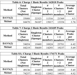
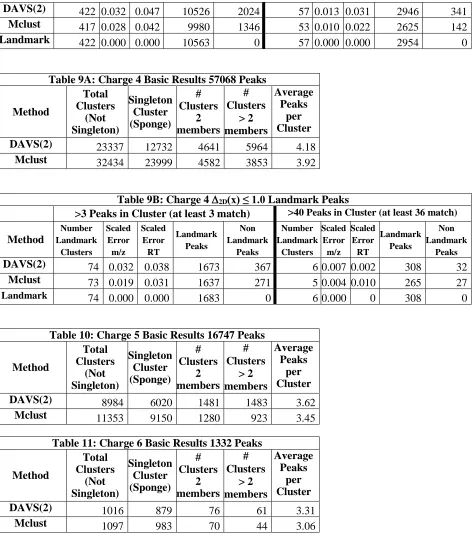
[image:13.612.71.395.295.610.2]

In tables 6-11, we record comparative results for DAVS(2) and Mclust for basic clustering statistics for charge z= 1 to 6. The rightmost column in tables 6, 7, 8A, 9A, 10 and 11gives the average number of peaks per cluster excluding singletons (“clusters” with one member or the sponge for DAVS(2)). Tables 8B and 9B give the Landmark peak analysis for charges 3 and 4 where there are significant data. As in charge 2 case, DAVS determines more clusters than Mclust.

Table 6: Charge 1 Basic Results 162818 Peaks

Method Total Clusters (Not Singleton) Singleton Cluster (Sponge) # Clusters 2 members # Clusters > 2 members Average Peaks per Cluster

DAVS(2) ₅₅₀₀₈ ₂₂₃₂₃ ₁₁₃₁₆ ₂₁₃₆₉ _4.3

Mclust ₈₄₄₇₈ ₅₆₁₀₇ ₁₅₀₁₇ ₁₃₃₅₄ _3.76

DAVS(2) ₅₄₀₅₄ ₁₉₄₄₉ ₁₀₈₂₄ ₂₃₇₈₁ _6.42

Mclust ₈₄₂₁₉ ₅₀₆₈₉ ₁₄₂₉₃ ₁₉₂₃₇ _5.69

Table 8A: Charge 3 Basic Results 174171 Peaks

DAVS(2) ₄₉₁₃₆ ₂₁₀₅₇ ₉₄₉₀ ₁₈₅₈₉ _5.45

[image:13.612.84.549.646.713.2]

Mclust ₇₄₂₅₇ ₄₈₁₂₂ ₁₂₀₈₂ ₁₄₀₅₃ _4.82

Table 8B: Charge 3 ∆2D(x) ≤ 1.0 Landmark Peaks

>3 Peaks in Cluster (at least 3 match) >40 Peaks in Cluster (at least 36 match)

(14)

DAVS(2) _{422 0.032 0.047} ₁₀₅₂₆ ₂₀₂₄ _{57 0.013 0.031} ₂₉₄₆ ₃₄₁ Mclust _{417 0.028 0.042} ₉₉₈₀ ₁₃₄₆ _{53 0.010 0.022} ₂₆₂₅ ₁₄₂

[image:14.612.73.545.70.605.2]

Landmark _{422 0.000 0.000} ₁₀₅₆₃ ₀ _{57 0.000 0.000} ₂₉₅₄ ₀

Table 9A: Charge 4 Basic Results 57068 Peaks

DAVS(2) ₂₃₃₃₇ ₁₂₇₃₂ ₄₆₄₁ ₅₉₆₄ _4.18

Mclust ₃₂₄₃₄ ₂₃₉₉₉ ₄₅₈₂ ₃₈₅₃ _3.92

Table 9B: Charge 4 ∆2D(x) ≤ 1.0 Landmark Peaks

>3 Peaks in Cluster (at least 3 match) >40 Peaks in Cluster (at least 36 match)

Method Number Landmark Clusters Scaled Error m/z Scaled Error RT Landmark Peaks Non Landmark Peaks Number Landmark Clusters Scaled Error m/z Scaled Error RT Landmark Peaks Non Landmark Peaks

DAVS(2) _{74 0.032 0.038} ₁₆₇₃ ₃₆₇ _{6 0.007 0.002} ₃₀₈ ₃₂

Mclust _{73 0.019 0.031} ₁₆₃₇ ₂₇₁ _{5 0.004 0.010} ₂₆₅ ₂₇

Landmark _{74 0.000 0.000} ₁₆₈₃ ₀ _{6 0.000} ₀ ₃₀₈ ₀

DAVS(2) ₈₉₈₄ ₆₀₂₀ ₁₄₈₁ ₁₄₈₃ _3.62

Mclust ₁₁₃₅₃ ₉₁₅₀ ₁₂₈₀ ₉₂₃ _3.45

DAVS(2) ₁₀₁₆ ₈₇₉ ₇₆ ₆₁ _3.31

Mclust ₁₀₉₇ ₉₈₃ ₇₀ ₄₄ _3.06

4 References

1. Rudolf Fruhwirth, D. Mani, and Saumyadipta Pyne, Clustering with position-specific constraints on variance: Applying redescending M-estimators to label-free LC-MS data analysis. BMC Bioinformatics, 2011. 12(1): p. 358. http://www.biomedcentral.com/1471-2105/12/358

2. Ken Rose, Eitan Gurewitz, and Geoffrey Fox, A deterministic annealing approach to clustering. Pattern Recogn. Lett., 1990. 11: p. 589--594.

(15)

3. Kenneth Rose, Eitan Gurewitz, and Geoffrey C Fox, Statistical mechanics and phase transitions in clustering. Phys. Rev. Lett., Aug, 1990. 65: p. 945--948.

4. Ken Rose, Deterministic Annealing for Clustering, Compression, Classification, Regression, and Related Optimization Problems. Proceedings of the IEEE, 1998. 86: p. 2210--2239.

5. Geoffrey C. Fox, Large scale data analytics on clouds, in Proceedings of the fourth international workshop on Cloud data management. 2012, ACM. Maui, Hawaii, USA. pages. 21-24.

http://grids.ucs.indiana.edu/ptliupages/publications/CloudDB12.pdf. DOI: 10.1145/2390021.2390026.

6. Yang Ruan, Saliya Ekanayake, Mina Rho, Haixu Tang, Seung-Hee Bae, Judy Qiu, and Geoffrey Fox, DACIDR: Deterministic Annealed Clustering with Interpolative Dimension Reduction using Large Collection of 16S rRNA Sequences, in ACM Conference on Bioinformatics, Computational Biology and Biomedicine (ACM BCB). October 7-10, 2012. Orlando, Florida.

http://grids.ucs.indiana.edu/ptliupages/publications/DACIDR_camera_ready_v0.3.pdf.

7. Geoffrey C. Fox, Deterministic annealing and robust scalable data mining for the data deluge, in Proceedings of the 2nd international workshop on Petascale data analytics: challenges and opportunities. 2011, ACM. Seattle, Washington, USA. pages. 39-40.

http://grids.ucs.indiana.edu/ptliupages/publications/pdac24g-fox.pdf. DOI: 10.1145/2110205.2110214.

8. Geoffrey Fox, Xiaohong Qiu, Scott Beason, Jong Youl Choi, Mina Rho, Haixu Tang, Neil Devadasan, and Gilbert Liu, Biomedical Case Studies in Data Intensive Computing, in The 1st International Conference on Cloud Computing (CloudCom 2009). December 1-4, 2009, Springer Verlag LNCS: Vol. 5931. Beijing Jiaotong University, China.

http://grids.ucs.indiana.edu/ptliupages/publications/SALSACloudCompaperOct10-09.pdf. 9. Geoffrey Fox, Seung-Hee Bae, Jaliya Ekanayake, Xiaohong Qiu, and H. Yuan, Parallel Data

Mining from Multicore to Cloudy Grids. book chapter of High Speed and Large Scale Scientific Computing. 2009: IOS Press, Amsterdam.

http://grids.ucs.indiana.edu/ptliupages/publications/CetraroWriteupJune11-09.pdf. ISBN:978-1-60750-073-5

10. Geoffrey Fox, Robust Scalable Visualized Clustering in Vector and non Vector Semimetric Spaces. Parallel Processing Letters, May 17, 2013. To be published.

http://grids.ucs.indiana.edu/ptliupages/publications/Clusteringv1.pdf

11. Hofmann, T. and J.M. Buhmann, Pairwise Data Clustering by Deterministic Annealing. IEEE Transactions on Pattern Analysis and Machine Intelligence, 1997. 19(1): p. 1-14.

12. J.Ekanayake, H.Li, B.Zhang, T.Gunarathne, S.Bae, J.Qiu, and G.Fox, Twister: A Runtime for iterative MapReduce, in Proceedings of the First International Workshop on MapReduce and its Applications of ACM HPDC 2010 conference June 20-25, 2010. 2010, ACM. Chicago, Illinois. http://grids.ucs.indiana.edu/ptliupages/publications/hpdc-camera-ready-submission.pdf.

13. Bingjing Zhang, Yang Ruan, Tak-Lon Wu, Judy Qiu, Adam Hughes, and Geoffrey Fox, Applying Twister to Scientific Applications, in CloudCom 2010. November 30-December 3, 2010. IUPUI Conference Center Indianapolis.

http://grids.ucs.indiana.edu/ptliupages/publications/PID1510523.pdf.

14. Thilina Gunarathne, Bingjing Zhang, Tak-Lon Wu, and Judy Qiu, Scalable Parallel Computing on Clouds Using Twister4Azure Iterative MapReduce Future Generation Computer Systems 2012. To be published.

http://grids.ucs.indiana.edu/ptliupages/publications/Scalable_Parallel_Computing_on_Clouds_Us ing_Twister4Azure_Iterative_MapReduce_cr_submit.pdf

15. Chris Fraley and Adrian E. Raftery, Enhanced Model-Based Clustering, Density Estimation, and Discriminant Analysis Software: MCLUST. Journal of Classiﬁcation, 2003. 20: p. 263-286. DOI:10.1007/s00357-003-0015-3.

http://www.stat.washington.edu/raftery/Research/PDF/fraley2003.pdf

16. Open Sysem Lab Indiana University Bloomington. MPI.NET Message Passing for C#. 2008 Available from: http://osl.iu.edu/research/mpi.net/.

17. Judy Qiu and Seung-Hee Bae, Performance of Windows Multicore Systems on Threading and MPI Concurrency and Computation: Practice and Experience, 2011. Special Issue for FGMMS

(16)

Frontiers of GPU, Multi- and Many-Core Systems 2010.

http://grids.ucs.indiana.edu/ptliupages/publications/CCPESpecialIssue_PerformanceofWindows MulticoreSystemsonThreadingandMPI.pdf