Generalized linear mixed models for count data

(1)

Generalized linear mixed models

for count data

Qiuyi Li

Supervisor: Prof. Alan Welsh

Oct 25, 2017

(2)

(3)

Acknowledgements

First and foremost, I would like to thank my supervisor Prof. Alan Welsh. With-out his patience and considerable effort, this thesis would not be here. No word of thanks will be enough to convey my gratitude for your forbearance, inspiration, and guidance throughout my honours year.

To all my friends, thank you for your accompanying and always being supportive during the tough times.

(4)

(5)

Abstract

(6)

(7)

Introduction

The traditional linear statistical models (LMs) have been developed primarily for normally distributed data. The generalized linear models (GLMs [28]) extend LMs to include a broader class of of distributions, the exponential family, includ-ing those commonly used for counts, proportions, and skewed distributions. A further extension of the GLMs, the generalized linear mixed models (GLMMs [30]) involve the additional random effects accounting for the correlation of the data. The process from simple to complex models (i.e. from LMs to GLMMs) enables us to construct a statistical model with fewer constraints. InChapter 1, we will

begin by reviewing the basics of LMs and GLMs, to serve as a starting point for proceeding to the GLMMs.

(10)

InChapter 3, we will discuss the methods of modeling the overdispersion [16] in Poisson mixed models (the GLMMs there the conditional distribution of response variables condition on the random effects is assumed to be Poisson). In statistics, overdispersion refers to the presence of greater variability in a data set than would be expected based on a given statistical model. The presence of overdispersion is often encountered when fitting relatively simple parametric models. For example the Poisson distribution has only one free parameter λ, which does not allow the variance to be adjusted independently from the mean as we can in, say, normal distribution.

In Chapter 4, we will investigate the asymptotic properties of the estimators by increasing the cluster size and the number of clusters respectively. An application example will be given in Chapter 5.

(11)

Chapter 1 Statistical models

1.1 Linear model

A linear model (LM), the simplest statistical model, is based on the assumption that a response variable can be modeled as the mean plus an error term, where the mean can be expressed in terms of a linear combination of explanatory variables and associated parameters and each error term is assumed to be independent and identically normally distributed.

Letybe anN×1 vector of independent response variables, the model matrixX

be a known matrix of order N ×p describing the explanatory variables that we are interested in, and β be a p×1 vector of unknown parameters modeling the ‘effect’ of each factor in X. We also call β the fixed effect parameters.

In general a linear model can be expressed in the form

y=µ+,

where µ=_E(y) = Xβ and ∼N(0, σ2_I

N) is the error vector.

For example, suppose there are 2 factors (f actor A, f actor B) that we are inter-ested, andyconsists of 3 components subject tof actor A, f actor B, f actors A and B

respectively, then we have:

y=    y1 y2 y3   , µ=

   µ1 µ2 µ3  

, X = 

 

1 1 0 1 0 1 1 1 1



 , β =

(12)

and    y1 y2 y3   =   

1 1 0 1 0 1 1 1 1

      β0 β1 β2   +    1 2 3   , or    µ1 µ2 µ3   =   

1 1 0 1 0 1 1 1 1

      β0 β1 β2   .

More explicitly, we have

µ1 =β0+ 1×β1 ⇒intercept+f actor A;

µ2 =β0+ 1×β2 ⇒intercept+f actor B;

µ3 =β0+ 1×β1 + 1×β2 ⇒intercept+f actor A+f actor B.

All the parametric statistical models are generalized from here.

1.2 Generalized linear model

A generalized linear model (GLM [29]) is a generalization of LMs, where the normality assumption for the response variables is replaced by a more general class of distribution, the exponential family. In the GLM, the distribution of the response variables is assumed to be from the exponential family of distributions which includes the normal distribution as a special case.

Definition 1.1 (Exponential family): LetX be a random variable with density functionfX(x|θ, φ). The exponential family is the set of probability distributions

with the density function of the form

fX(x|θ, φ) = exp{[xθ−b(θ)]/φ2+c(x, φ)}, (1.1)

whereb(·),c(·) are known functions, andθis often called the canonical parameter and φ the dispersion parameter.

The exponential family includes many of the most common distributions. For example the normal distribution

fX(x|µ, σ) =

1

√

2πσ2exp n

− (x−µ) 2

2σ2 o

= expnxµ−µ

2_/₂

σ2 −

1 2

hx2

σ2 + log(2πσ

(13)

where θ=µ,φ2 =σ2, b(θ) =µ2/2,c(x, σ) = [x2/σ2+ log(2πσ2)]/2. More interestingly the Poisson distribution,

gX(x|λ) =e−λ

λx x!

= exp{xlogλ−λ−log(x!)}

= exp{xθ−eθ−log(x!)} (θ= logλ), (1.3) where φ2 _≡_1, _b₍_θ_{) = exp(}_θ_), _c₍_{x, φ}_{) =}_c₍_x_{) =} ₋_log(_x_!).

Theorem 1.1: For a random variable X with the distribution function of the form (1.1), then under regularity conditions which allows us to take partial deriva-tives outside the integral [14], we have

E(X|θ, φ) =b0(θ); (1.4)

var(X|θ, φ) =b00(θ)φ2. (1.5)

Proof: We have

d

dθfX(x|θ, φ) =

x−b0(θ)

φ2 fX(x|θ, φ) ⇒

Z _d

dθfX(x|θ, φ)dx=

Z _x₋_b0₍_θ₎

φ2 fX(x|θ, φ)dx ⇒ d

dθ

Z

fX(x|θ, φ)dx=

1

φ2 Z

[x−b0(θ)]fX(x|θ, φ)dx.

Since R fX(x|θ, φ)dx= 1 by the definition of density function, we have

d dθ

Z

fX(x|θ, φ)dx=

d

dθ1 = 0.

Therefore,

b0(θ)

Z

fX(x|θ, φ)dx =

Z

xfX(x|θ, φ)dx,

b0(θ) =_E(X|θ, φ).

Also,

d2

dθ2fX(x|θ, φ) =

−b00(θ)

φ2 fX(x|θ, φ) +

hx−b0(θ)

φ2 i2

fX(x|θ, φ)

⇒ Z

d2

dθ2fX(x|θ, φ)dx=

Z _n₋

b00(θ)

φ2 +

hx2+b0(θ)2 −2xb0(θ)

φ4

io

fX(x|θ, φ)dx

⇒ d 2

dθ2 Z

fX(x|θ, φ)dx=

Z

n−b00(θ)

φ2 +

hx2+b0(θ)2 −2xb0(θ)

φ4

io

(14)

As above, we have

b00(θ)φ2

Z

fX(x|θ, φ)dx=

Z h

x2+b0(θ)2−2xb0(θ)ifX(x|θ, φ)dx,

b00(θ)φ2 =_E(X2|θ, φ) +_E2(X|θ, φ)−2_E2(X|θ, φ), b00(θ)φ2 =var(X|θ, φ),

as required.

In a GLM, a non-identity link function g(·) is introduced so that the mean of response variables (µ) is no longer always a linear combination of the columns of

X, but instead acts on a scale as dictated by the link function, i.e.

µ=g−1(Xβ) =g−1(η)

where η = g(µ) = Xβ. Using the same example from above, where we have 2 distinct factors and 3 response variables. We define

η = [g(µ1), g(µ2), g(µ3)]T,

then



 

g(µ1)

g(µ2)

g(µ3) 

 =



 

1 1 0 1 0 1 1 1 1



 



 

β0

β1

β2 

 ,

or equivalently

g(µ1) = β0 + 1×β1 ⇒intercept+f actor A;

g(µ2) = β0 + 1×β2 ⇒intercept+f actor B;

g(µ3) = β0 + 1×β1+ 1×β2 ⇒intercept+f actor A+f actor B.

1.3 Generalized linear mixed model

(15)

The terms fixed and random effects are used in the context of mixed models. Before introducing the fixed and random effects, we first distinguish between the fixed and random variables:

Fixed and random variables

(i) A fixed variable is one that is assumed to be measured without error. It is also assumed that the values of a fixed variable in one study are the same as the values of the fixed variable in another study and will remain consistent across different studies.

(ii) Random variables are assumed to be values that are drawn from a larger population of values and thus will represent them, which can be thought of as representing a random sample of all possible values or instances of that variable. Thus, we expect to generalize the results obtained with a random variable to all other possible instances of that value.

Fixed and random effects

(i) Fixed effect: In general, a fixed effect refers to the effect which is assumed to be a fixed variable. The fixed effect can be generalized to the population or other studies exposed to the same effect.

(ii) Random effect: Similarly, a random effect is the effect which is assumed to be a random variable. In general, the random effects are used if the levels of the random effects are thought to be a small subset of all the possible values that one wishes to generalize to. Such a generalization is more of an inferential leap, and consequently, the random effects model will produce larger standard errors compared to the fixed effects model.

(16)

In general, whether a certain effect should be considered as fixed or random need to be determined in each particular case.

Cluster sampling

Cluster sampling refers to a type of sampling method . With cluster sampling, the researcher divides the population into separate groups, called clusters. Then, a simple random sample of clusters is selected from the population. The researcher conducts his analysis on data from the sampled clusters. As in the previous ex-ample, the 10 schools randomly chosen by the researcher are the clusters.

We denote the (q × 1) vector of random effects as u, and the corresponding model matrix Z of order (N ×q). Let yi ∈ y, 1 ≤ i ≤ N be an arbitrary

response variable in y, we assume

yi|u∼indep. f(yi|u),

i.e. the response variables are conditionally independent.

Let λ=_E(y|u),g(·) be the link function as in GLMs, we have

η0 =Xβ+Zu

where η0 =g(λ).

To illustrate this, we augment the previous example so that y can be split into 2 clusters (y1 in cluster 1, and the other two in cluster 2) and there exists 1 random

factor within each cluster (rand 1, rand 2). For convenience, we rewrite y1 as

y1,1 indicating that it is the 1st component in cluster 1. Likewise we write y2 as

y2,1, y3 as y2,2.

Moreover, we define

λ=



 

λ1,1

λ2,1

λ2,2 

 , η

0

=



 

g(λ1,1)

g(λ2,1)

g(λ2,2) 



, Z =    1 0 0 1 0 1   , u=

" u1 u2 # , then likewise   

g(λ1,1)

g(λ2,1)

g(λ2,2)   =   

1 1 0 1 0 1 1 1 1

(17)

equivalently,

g(λ1,1) = β0+ 1×β1+ 1×u1 ⇒intercept+f actor A+rand 1;

g(λ2,1) = β0+ 1×β2+ 1×u2 ⇒intercept+f actor B+rand 2;

g(λ2,2) = β0+ 1×β1+ 1×β2+ 1×u2 ⇒intercept+f actor A+f actor B+rand 2.

To complete the specifications, we assign a distribution to random effects such that u∼k(u), with mean0 and covariance matrix Γ.

Properties of GLMMs:

(i) Marginal expectations 6= conditional expectation:

Let yij be an arbitrary response variable in y and let ui be the random

effects for cluster i. Then we have

η0_ij =g(λij) = xTijβ+z T ijui,

so the conditional expectation

λij =g−1(xTijβ+z T ijui).

where xij and uij are respectively the rows of X and Z corresponding to

yij, written in column vectors.

The marginal expectation is

µij =E(λij) =E[g−1(xTijβ+z T ijui)].

For example, supposeyij|u∼P oisson(λij),g(·) = log(·) andui ∼M V N(0,Γ).

Then

λij = exp(xTijβ+z T

ijui); (1.6)

µij =E[exp(xTijβ+z T ijui)]

= exp(xT_ijβ+z_ijTΓzij/2). (1.7)

If ui =ui ∼N(0,1) andzij = 1, this can be further simplified to

λij = exp(xTijβ+ui);

µij = exp(xTijβ+ 1/2),

(18)

(ii) Marginal variance 6= conditional variance:

Let δ_ij2 =var(yij|u), and σij2 =var(yij), then

δ_ij2 =_E[y_ij2]−λ2_ij; (1.8)

σ_ij2 =_E[δ_ij2] +var[λij]. (1.9)

Equality holds only in trivial case where var[λij] = 0, i.e. λij =µij, which

means there is no random effect. Hence the GLMM is reduced to a GLM.

Moreover, since the distribution function of yij belongs to the exponential

family, then from (1.4), we have

δ_ij2 =b00(θij)φ2;

σ_ij2 =_E[δ2_ij] +var[λij]

=_E[b00(θij)φ2] +var[b0(θij)]

(19)

Chapter 2 Methods of estimation

To avoid ambiguity, we let yij, j = 1,2, ..., ni,be thejth response variable within

ith cluster,yi = (yi1, yi2, ..., yini)

T_{, i}_{= 1}_,₂_{, ..., c,}_{be the (}_n

i×1) vector of response

variables in the ith cluster andy = (y1,y2, ...,yc)T denotes the (N×1) vector of

response variables.

Moreover, we define β to be a (p× 1) vector of fixed effect parameters, and let ui = (ui1, ui2, ..., uiq)T, i= 1,2, ..., c, be a (q×1) vector of the random effect

corresponding to the ith cluster. We denote u = (u1,u2, ...,uc)T as an (qc×1)

vector of random effects.

Likewise, we denote the (N ×p) fixed-effect model matrix by X, the (ni ×p)

fixed-effect model matrix corresponding toithcluster byXi, and the (p×1)

fixed-effect model vector corresponding toyij byxij, and similarly for the random-effect

model matrix Z.

We consider the following model:

(i) Foryij ∈y, we have yij|u∼indep. f(yij|u) with

f(yij|u) = exp[yijθij0 −b(θ

0

ij)]/φ

2 ₊_c₍_y

ij, φ),

as in exponential family, then the joint density

f(y|u) =Y

i,j

exp[yijθij0 −b(θ

0

ij)]/φ

2₊_c₍_y

ij, φ)]

= exp[yTθ0−B(θ0)]/φ2 +C(y, φ)], (2.1) which is the exponential family in the vector-parameter form over a vector of random variables, whereB(θ0) = P

i,jb(θ

0

ij) and C(y, φ) =

P

(20)

Then the conditional log-likelihood of y given u has the GLM form:

l(θ0, φ,y|u) = [yTθ0−B(θ0)]/φ2+C(y, φ), (2.2) Notice from above that we denote µ0 =_E(y|u) and η0 =g(µ0), where g(·) is the link function. The linear predictor η0 takes the form

η0 =η+v(u), (2.3)

where η=Xβ and v(u) =Zu.

(ii) The distribution ofu is assumed appropriately and also in the exponential family.

The modeling of η0 in (2.3) involves not only the fixed effects modeling forη, but also the random effects modeling for u.

2.1 Ordinary likelihood function

From the definition of a GLMM, we have

yij|u∼indep. f(yij|u)

Moreover, under most circumstances, we assume that the random effects are in-dependent among clusters, i.e. ui’s are mutually independent. For mathematical

convenience, we often assume further that ui ∼ iid M V N(0,Γ), where Γ is the

covariance matrix. Then

u∼k(u) =

c

Y

i=1

k(ui).

Therefore we can write the likelihood function as

L(y,β) =

c

Y

i=1

ni

Y

j=1

f(yij)

=

Z c Y

i=1

ni

Y

j=1

f(yij|u,β)k(u)du

=

Z

(21)

where

h(y,β,u) = log[

c

Y

i=1

ni

Y

j=1

f(yij|u,β)k(u)]

=X

i,j

logf(yij|u,β) + logk(u)

= logf(y|u,β) + logk(u), (2.5)

which is called the hierarchical-likelihood [25], and will be discussed further in the following section.

Due to the involvement of integration, the ordinary likelihood function can be hard to obtain. For example, even for the very simple case where we assume

ni = 1, i= 1,2, ..., c, and

yi|u∼P oisson(λi);

logλi =xTi β+ui;

ui ∼i.i.d. N(0,1),

then

f(yi|u,β) = exp[yi(xTi β+ui)−exp[xTi β+ui]−log(yi!)],

so

h(y,β,u) =yi(xTiβ+ui)−exp[xTi β+ui]−log(yi!).

Hence the likelihood function is of the form

Z c Y

i=1

f(yi|u,β)k(u)du = c

Y

i=1 Z

f(yi|ui,β)k(ui)dui

=

c

Y

i=1 Z

exp[yi(xTi β+ui)−exp[xTi β+ui]−log(yi!)

−1

2(u

2

i + log 2π)]dui,

which is intractable! Thus in order to obtain parameter estimates, we either need to approximate the likelihood function or find a good substitute of it.

2.2 Hierarchical-likelihood

By the properties of exponential family, we have µ0 =B0(θ0), then

(22)

We assume that B0(·) is invertible, thus from (2.6) we can write θ0 as a function of β and u.

Definition 2.1: The hierarchical-likelihood [25], denoted by h is defined by

h= logf[y,θ0(β,u), φ,σ]

= logf[y,θ0(β,u), φ|u] + logk(σ,u)

where θ0 is canonical parameters and σ,φ are dispersion parameters. We denote

ψ = (θ0, φ). Thus we can rewrite the h-likelihood as

h= logf(y,ψ|u) + logk(u,σ) (2.7)

In this case, we treat the random effectsuthe same as the fixed effect parameters

β, i.e. instead of only being interested in the variance of u as in many of the other methods, we also compute the estimates of u. Equivalently, we are now fitting c(number of clusters) GLMs.

2.2.1 Theory

The maximum h-likelihood estimates can be obtained by solving

∂h(y,ψ,u,σ)

∂β =0, (2.8)

∂h(y,ψ,u,σ)

∂u =0. (2.9)

If we choose the link function g(·) =B0(·), we have

η0 =θ0.

Substituting into (2.3), we have

θ0_ij =θij +zTijui, (2.10)

Moreover,

∂θ_ij0 ∂βk

= ∂

P

lxijlβl

∂βk

=xijk;

∂θ0_ij ∂uik

= ∂

P

lzijluil

∂uik

(23)

Then using chain rule, we have

∂h(y,ψ,u,σ)

∂βk

= ∂h(y,ψ,u,σ)

∂θ0

∂βk

=

P

i,j[yij−b

0₍_θ0

ij)]xijk

φ2

=

P

i,j[yij−λij]xijk

φ2

= 0, k= 1,2, ...p. (2.11)

We assume further that ui ∼M V N(0,Γ), then similarly

∂h(y,ψ,u,σ)

∂uik

= ∂

∂uik

P

i,jyijθ0ij−b(θ

0

ij) +

P

i,m,nuimΓ−mn1uin/2

φ2

=

P

j[yij −λij]zijk+

P

nΓ

−1

knuin+ Γ

−1

kkuik

φ2

= 0, k= 1,2, ..., q. (2.12)

If we assume furthermore that the random effects are independent, Γij =σ2iχ{i=j},

we have the simple estimating equation

∂h(y,ψ,u,σ)

∂uik

=

P

j[yij −λij]zijk+uik/σ

2

k

φ2 = 0. (2.13)

The h-likelihood can not be used to estimate the variance components of the random effects. For example, if we try to compute

∂h(y,ψ,u,σ)

∂σk

= 0, k = 1,2, ..., q, (2.14)

we will have σk → ∞, which is clearly not what we want. However, we can

approximate the variance components by the sample variance (covariance) of the estimates of the random effects. For example

ˆ

σk =sk =

1 c c X i=1 ˆ

u2_ik. (2.15)

2.2.2 Discussion

(24)

In the next section, we are going to discuss the method of Laplace approximation, which in some sense is quite similar to the hierarchical-likelihood with lower risk of overfitting.

2.3 Laplace approximation

2.3.1 Background

The integral in the likelihood function for a glmm can be written in the form [37],

I =

Z

Rq

exp[−N s(u)]du, (2.16)

in which n is the sample size. In the standard asymptotic regime, q is invariant as N → ∞, while in non-standard high dimensional cases, it is possible for q to increase with N, which will make the evaluation process harder of maybe even impossible at present.

In the classic application of Laplace approximation, we expand the natural log of the integrand in a second-order Taylor series around the maximum point (first-order derivatives equal to zero), and under certain regularity conditions, the higher order terms decay to zero as N gets large, making the approximation accurate in large samples, i.e. we approximate h(u) :=−N s(u) by

ˆ

h(u)≈h( ˆu)− 1

2 q X i=1 q X j=1 h − ∂ 2_h

∂ui∂uj

i

u= ˆu

(ui−uˆi)(uj−uˆj)

=h( ˆu)− 1

2 q X i=1 q X j=1

V_ij−1(ui−uˆi)(uj−uˆj), (2.17)

where

V_ij−1 =h− ∂ 2_h

∂ui∂uj

i

u= ˆu.

Then the integral I can be approximated by

ˆ

I = exp[h( ˆu)]

Z

exph−(u−uˆ)

T_V−1₍_u₋_u_ˆ₎

2

i

du

= (2π)n2 exp[h( ˆu)]

√

(25)

provided that V is positive definite.

In this thesis, we will generalize this idea to higher order Laplace approxima-tion, which can approximate the integral more accurately even when the sample size is relatively small. We will propose a multivariate Taylor series approxima-tion of the log of the integrand that can be made as accurate as desired if the integrand and all its derivatives with respect to u are continuous. Finally for application, we will balance between the accuracy and complexity (computation time) to give the optimal order in which the Laplace approximation is remarkably accurate and computationally fast in comparison with other methods.

2.3.2 Theory

Standard regularity conditions

For the following theories to be valid, there are certain regularity conditions need to be satisfied:

(i) q remains constant as n increases.

(ii) s(·) is unimodal with a minimum at ˆu.

(iii) the integral is exponentially small outside any fixed interval containing ˆu.

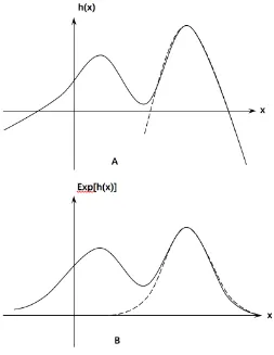
where the last two conditions ensure that the main contribution of the integrand comes from x-values in ano(1) neighborhood of ˆu. The following figures provide an intuitive explanation for the importance of the last two conditions, by giving a counterexample.

As in Figure 2.1, neither is g(·) unimodal nor the integral is sufficiently small outside any fixed interval containing ˆu and clearly, the (standard) Laplace ap-proximation indicated using dashed line fails to give a good fit to the integrand.

(26)

[image:26.595.150.403.80.407.2]

Figure 2.1

Multivariate Taylor series expansion

Definition 2.2 (Infinite multivariate Taylor series): Let h(u) be a scalar func-tion of a vector u, with all its partial derivatives continuous in a neighborhood

N of ˆu, then for u in N, we have

h(u) =h( ˆu) +h(1)( ˆu)(u−uˆ) + 1

2(u−uˆ)

T_h(2)_{( ˆ}_u₎₍_u₋_u_ˆ₎

+ 1

3![(u−uˆ)

T _⊗₍_u₋_u_ˆ₎T_]_h(3)_{( ˆ}_u₎₍_u₋_u_ˆ_{) +}_...

+ 1

n![⊗

n−1₍_u₋_u_ˆ₎T_]_h(n)_{( ˆ}_u₎₍_u₋_u_ˆ_{) +}_...

=h( ˆu) +h(1)( ˆu)(u−uˆ) +

∞

X

k=2

1

k![⊗

k−1₍_u₋_u_ˆ₎T_]_h(k)_{( ˆ}_u₎₍_u₋_u_ˆ₎_, _(2.19)

where

h(k)( ˆu) = ∂ vec[h

(k−1)₍_u_)]

∂ uT

u= ˆu

(27)

and ⊗ denotes the Kronecker product.

Noticing that h(u) equals to its infinite multivariate Taylor series expansion around ˆu under regularity conditions. We have not done any ‘approximation’ yet. We now compute the integral R

Rqexp[h(u)]du by replacing h(u) with its infinite Taylor series, where we have the theorem:

Theorem 2.1: [35] Suppose h(u) has a maximum at u = ˆu, then for any

u∈_Rq_{, we have}

Z

Rq

exp[h(u)]du= (2π)q/2|V|1/2_exp[_h_{( ˆ}_u_)]_×

E[exp(R)], (2.21)

where _E(·) denotes the expectation taken over the multivariate normal distribu-tion with mean0, and covariance matrix V = [−h(2)( ˆu)]−1, which is assumed to be positive definite andR =P∞

k=3Tk withTk= _k1_![⊗k−1(u−uˆ)T]h(k)( ˆu)(u−uˆ).

Proof: We have h(1)( ˆu) = 0 since ˆu maximizes h(u) by assumption. Then we can rewrite the integral as

Z

Rq

exp[h(u)]du= exp[h( ˆu)]

Z

Rq

exp[−1

2(u−uˆ)

T_V−1₍_u₋_u_ˆ_{)] exp[}_R_]_d_u

= (2π)q/2|V|1/2_exp[_h_{( ˆ}_u_)]_×

E[exp(R)]

as required.

To evaluate _E[exp(R)], we apply the infinite Taylor series once again to exp[R] so we have

E[exp(R)] = E[

∞

X

k=0

Rk

k!] =

∞

X

k=0 E[Rk]

k! (2.22)

So far, we have kept carrying the infinite Taylor series, so any result is strictly accurate. While it is not feasible to propose a general formula for computing

E[Rk], this is the point where approximation comes in.

Approximation to o(N−2₎

(28)

(i) h(·) and all of its derivatives areO(N) by the definition ofh(·), and later on we will see that this property is preserved by the integrand of the likelihood function in GLMMs.

(ii) (ui−uˆi) isO(N−1/2) for alli, by the assumption thatufollows a multivariate

normal distribution centered at ˆu, hence the standard deviation of each component is O(N−1/2_).

(iii) By definition, Tk ∼O(N1−k/2) fork ≥3.

(iv) R = P∞

k=3Tk has the same order with the leading term T3, hence R ∼

O(N−1/2_).

Before we introduce the generalized Laplace approximation, we consider first the relative error of the standard Laplace approximation. We have the lemma:

Lemma 2.1: The standard Laplace approximation (2.17) has relative erroro(1).

Proof: In the standard Laplace method, we approximate h(x) by its second order Taylor expansion as in (2.17). Together with the properties above, we have

h(u) =h( ˆu)− 1

2

X

ij

h − ∂

2_h

∂ui∂uj

i

u= ˆu(ui−uˆi)(uj−uˆj) +o(1)

=h( ˆu)− 1

2(u−uˆ)

T_V−1₍_u₋_u_ˆ_{) +}_o₍₁₎_.

Then by Theorem 2.1, we have

Z

Rq

exp[h(u)]du= exp[h( ˆu)]

Z

Rq

exp[−1

2(u−uˆ)

T

V−1(u−uˆ)] exp[o(1)]du

= (2π)p/2|V|1/2_exp[_h_{( ˆ}_u_)]_×_{[1 +}_o_(1)]

= (2π)p/2|V|1/2exp[h( ˆu)] +o(1). (2.23)

Hence the error term decays slowly given larger sample size, which explains why the standard Laplace approximation doesn’t work quite well in practice and there-fore, we should expect a considerable improvement in accuracy if we can approx-imate the integral to higher order.

(29)

one can easily generalize this to arbitrarily high order using the same idea. First we approximate R to the 6th order, which gives

R = T3 +T4 +T5 +T6 +o(N−2)

O(N−1/2) O(N−1) O(N−3/2) O(N−2) Then we approximate exp(R) to the 4th order:

exp(R) = 1 +R +R

2

2 +

R3

3! +

R4

4! +o(N

−2₎

O(1) O(N−1/2) O(N−1) O(N−3/2) O(N−2) When combining them, we find the following theorem useful:

Theorem 2.2: [35]

E[TiTj...Tk] = 0, for odd (i+j+...+k), i, j, ..., k ∈N≥3; (2.24) E[TiTj...Tk] =

[(i+j +...+k)−1][(i+j+...+k)−3]...3 (i!j!...k!)

×vecT(⊗(i+j+...+k)/2_V₎_vec_[_h(i)_{( ˆ}_u₎_⊗_h(j)_{( ˆ}_u₎_⊗_..._⊗_h(k)_{( ˆ}_x_)]_,

for even(i+j+...+k), i, j, ..., k ∈_N≥3. (2.25)

Proof: SinceTk is a scalar, we have [27]

E(Tk) = E h1

k![⊗

k−1

(u−uˆ)T]h(k)( ˆu)(u−uˆ)

i

= 1

k!vec

T

E n

[⊗k−1(u−uˆ)](u−uˆ)T

o

vec[h(k)( ˆu)].

Likewise,

E(TiTj...Tk) =

vecT

E

n

[⊗(i+j+k)−1₍_u₋_u_ˆ_)](_u₋_u_ˆ₎To_vec_[_h(i)_{( ˆ}_u₎_⊗_h(j)_{( ˆ}_u₎_⊗_..._⊗_h(k)_{( ˆ}_u_)]

i!j!...k! ,

where _E{[⊗(i+j+k)−1₍_u₋ _u_ˆ_)](_u ₋_u_ˆ₎T_} _:= _µ

(i+j+...+k) is the (i+j +...+k)th

moment of the multivariate normal distribution with covariance matrix V and

µ(i+j+...+k) =0 for odd (i+j+...+k).

When (i+j+...+k) is even, we have [50]

(30)

where S is any conformable matrix of constant. Therefore

E[TiTj...Tk] =

[(i+j +...+k)−1][(i+j+...+k)−3]...3 (i!j!...k!)

×vecT(⊗(i+j+...+k)/2V)vec[h(i)( û)⊗h(j)( û)⊗...⊗h(k)( û)],

as required.

Hence we have

exp(R) = 1

+T4+T6+o(N−2)

+1

2(T

2 3 +T

2

4 +T3T5) +o(N−2)

+ 1

3!T

2

3T4+o(N−2)

+ 1

4!T

4

3 +o(N

−2₎

= 1 +T4+T6+

1 2(T

2 3 +T

2

4 +T3T5) +

1 3!T

2 3T4+

1 4!T

4

3 +o(N

−2₎_. _(2.26)

Taking expectation on both sides, we have

E[exp(R)] = 1

+ 3

4!vec

T₍_V _⊗_V₎_vec_[_h(4)_{( ˆ}_u_{)] +} 5×3

6! vec

T₍_⊗3_V₎_vec₍_h(6)_{[ ˆ}_u_)]

+1

2

n5×3

3!3! vec

T₍_⊗3_V₎_vec_[_h(3)_{( ˆ}_u₎_⊗_h(3)_{( ˆ}_u_)]

+7×5×3

4!4! vec

T₍_⊗4_V₎_vec_[_h(4)_{( ˆ}_u₎_⊗_h(4)_{( ˆ}_u_)]

+7×5×3

5!3! vec

T₍_⊗4_V₎_vec_[_h(3)_{( ˆ}_u₎_⊗_h(5)_{( ˆ}_u_)]o

+ 1

3!

n9×7×5×3

3!3!4! vec

T₍_⊗5_V₎_vec_[_h(3)_{( ˆ}_x₎_⊗_h(3)_{( ˆ}_u₎_⊗_h(4)_{( ˆ}_u_)]o

+ 1

4!

n11×9×7×5×3

3!3!3!3! vec

T₍_⊗6_V₎_vec_[_h(3)_{( ˆ}_x₎_⊗_h(3)_{( ˆ}_u₎_⊗_h(3)_{( ˆ}_x₎_⊗_h(3)_{( ˆ}_u_)]o

+o(N−2). (2.27)

Hence by substitution, the integral R

Rqexp[h(u)]du = (2π)

(31)

2.3.3 Application in GLMMs

Comparison to the hierarchical-likelihood

We are principally interested in approximating the likelihood function (2.4),

L(y,β) =

Z Y

i,j

f(yij|u,β)k(u)du

=

Z

exp[h(y,β,u)]du.

By the definition of Laplace approximation, we expand h(y,β,u) around its maximum ˆu, which is the root of

∂h(y,β,u)

∂u =0. (2.28)

This should be familiar to us, if we notice that this equation appears exactly in the estimation process for likelihood in (2.9). While in hierarchical-likelihood, we estimate β by solving

∂h(y,β,u)

∂β =0,

in Laplace approximation, we compute the integral first, using the Taylor series expansion ofharound ˆuto approximateh, and the differentiate the integral with respect to β to obtain the parameter estimates, i.e. we approximate L(y,β) by

ˆ

Lla(y,β) :=

Z

exp[h(y,β,u∗)]du= (2π)q/2|V|1/2_exp[_h_{( ˆ}_u_)]_×

E[exp(R)].

(2.29)

Then we can obtain the parameter estimates ˆβla by solving

∂Lˆla(y,β)

∂β =0. (2.30)

The variance of ˆβla can be estimated by the inverse of the Fisher information

matrix [13]:

d

var(β) =h−_E∂ 2_L_ˆ

la(y,β)

∂β∂βT

i−1 β= ˆβla

. (2.31)

(32)

Example

To avoid too much complexity, we will do a second order Laplace approximation as a demonstration. We have

L(y,β)≈Lˆla(y,β)

= (2π)q2 exp[h(y,β,uˆ)]

√

detV,

provided V is positive definite. The Laplace approximation estimator ˆβla is the

maximizer of ˆLla(y,β), which requires solving

∂Lˆla(y,β)

∂β =0;

⇒exp[h(y,β,uˆ)](h0_β

k(y,β,uˆ)

√

detV + ∂

∂βk

√

detV) = 0;

⇒h0_β

k(y,β,uˆ)

√

detV + ∂

∂βk

√

detV = 0.

Hence ˆβla is the root of

h0_β

k(y,β,uˆ)

√

detV + ∂

∂βk

√

detV = 0,

for k = 1,2, ..., p.

Now we consider the case where the response variables are assumed to follow the Poisson distribution. The model can be expressed as:

log(λij) = xTijβ+z T ijui

f(yij|u) = exp[yij(xTijβ+z T

ijui)−exp[xTijβ+z T

ijui]−log(yij!)]

Assume uik ∼N(0, σ2k) and are mutually independent, so

k(ui) =

q

Y

k=1

1

p

2πσ2

k

exph− u 2

ik

2σ2

k

i

= exph−

q X k=1 (u 2 ik

2σ2

k

+ 1

2log(2πσ

2

k))

i

.

Hence

hij(yij,β,ui) =yij(xTijβ+z T

ijui)−exp[xTijβ+z T ijui]−

q X k=1 (u 2 ik

2σ2

k

+ 1

2log(2πσ

2

(33)

and consequently

hi(yi,β,ui) = ni

X

j=1

hij(yij,β,ui);

h(y,β,u) =

m

X

i=1

hi(yi,β,ui).

where ni denotes the number of response variables in cluster iand cdenotes the

total number of clusters.

Solving for u∗:

∂h ∂uik

= ∂hi

∂uik = 0; ⇒ ni X j=1 ∂ ∂uik h

yij(xTijβ+z T

ijui)−exp[xTijβ+z T ijui]−

q

X

k=1

u2_ik

2σ2

k i = 0; ⇒ ni X j=1 h

yijzijk−zijkexp[xTijβ+z T ijui]−

q X k=1 uik σ2 k i = 0; ⇒ ni X j=1 h

yijzijk−zijkexp[xTijβ+z T ijui]

i −ni

q X k=1 uik σ2 k

= 0.

In order to get the solution for ˆui, we need to solve the system of q (number of

random effects in each cluster) equations for each i.

If we assume further that q = 1, u ∼ M V N(0,I), then the equation will be simplified to

ni

X

j=1 h

yijzij −zijexp[xTijβ+zijui]−niui = 0,

which still require numerical technique to obtain a numerical solution.

2.3.4 Discussion

(34)

In the previous section, we have developed some theories that allow us to approx-imate the integral to sufficiently high order (o(N−2) as illustrated). However, this dose not necessarily ensure higher accuracy in practice, especially when N

is relatively small. In this case, as is often the case in GLMMs, the coefficient of the error term will become important. For example, if N = 4 and the error term

R ≈104N−2, the result will be ridiculously inaccurate.

Unfortunately, the coefficient of the error term has to be determined for each particular case and is often hard to obtain. Although empirically Laplace ap-proximation works fine, it is still recommended that one should check for the range of the error term whenever applying the Laplace approximation.

One might be astonished by the complicated formula of the high order Laplace approximation. In the next section, we will discuss an alternative numerical ap-proximation method named Gauss-Hermite quadrature, which shares the same asymptotic properties with the high order Laplace approximation and can be used to estimate the variance components of the random effects, but is only applicable in simple cases.

2.4 Gauss-Hermite quadrature

Before we discuss Gauss-Hermite quadrature we introduce first the Newton-Cotes formulas [44].

2.4.1 Newton-Cotes formulas

In numerical analysis, the Newton-Cotes formulas, also called the Newton-Cotes quadrature rules or simply Newton-Cotes rules, are a group of formulas for nu-merical integration (also called quadrature) based on evaluating the integrand at equally spaced points. They are named after Isaac Newton and Roger Cotes. It is assumed that the value of a functionf(x) defined on [a, b] is known at equally spaced points xi, for i = 0, ..., n, where x0 = a and xn = b. The Newton-Cotes

formula of degree n is

Z b

a

ξ(x)dx≈

n

X

i=0

(35)

Later, we will write ξ(x) = w(x)f(x) for some weight function w(·).

Definition 2.3 (Lagrange basis polynomials): Given a set of n + 1 distinct data points

(x0, ξ(x0)), ...,(xn, ξ(xn)), then for 0≤j ≤n, the Lagrange basis polynomials are

defined as

`j(x) :=

Y

0≤i≤n, i6=j

x−xi

xj −xi

. (2.33)

One can easily check that `j(xi) =δij.

Definition 2.4 (Interpolation polynomial in the Lagrange form): The inter-polation polynomial in the Lagrange form is defined as a linear combination

L(x) :=

n

X

i=0

ξ(xi)`i(x), (2.34)

of Lagrange basis polynomials. It follows that L(xi) = ξ(xi), showing that L

interpolates f exactly.

Proof of Newton-Cotes formula: Let L(x) be the interpolation polyno-mial in the Lagrange form for the given data points (x0, f(x0)), ...,(xn, f(xn)),

then

Z b

a

ξ(x)dx≈ Z b

a

L(x)dx

=

Z b

a n

X

i=0

ξ(xi)`i(x)dx

=

n

X

i=0

ξ(xi)

Z b

a

`i(x)dx

=

n

X

i=0

wiξ(xi),

where wi :=

Rb

a `i(x)dx.

Note that if f(x) itself is a polynomial of degree less or equal to n, then

ξ(x) =

n

X

i=0

ξ(xi)`i(x),

(36)

It is important to note that in the derivation of the Newton-Cotes formulas we assumed that the nodes xi were equally spaced and fixed. The main idea for

ob-taining more accurate quadrature rules is to treat the nodes as additional degrees of freedom, and then hope to find ‘good’ locations that ensure higher accuracy.

Therefore, we now have n + 1 nodes xi in addition to n + 1 polynomial

coef-ficients for a total of 2n+ 2 degrees of freedom. This should be enough to derive a quadrature rule that is exact for polynomials of degree up to 2n+ 1, i.e. with the same amount of computation, we can improve the accuracy of the approxi-mation by sophisticatedly choosing different nodes.

Gaussian quadrature, indeed accomplishes this:

2.4.2 Gaussian quadrature

Gaussian quadrature is designed for computing integrals of the form

I(f) =

Z b

a

f(x)w(x)dx, (2.35)

where w(x) is a weight function on [a, b] (a, b∈_R∪ {±∞}), saitisfying

Z b

a

w(x)|x|n_{dx <}_∞_{, n}_{= 1}_,₂_,₃_{, ...}

In Gaussian quadrature, we approximate the integral by a weighted sum of func-tion values at specified points within the domain of integrafunc-tion, i.e.

I(f) =

Z b

a

f(x)w(x)dx≈

n

X

i=0

wif(xi), (2.36)

for some weight function (wi).

In fact we have the following theorem:

Theorem 2.3: Letqbe a nonzero polynomial of degreen+ 1 and w(·) a positive weight function such that

Z b

a

xkq(x)w(x)dx= 0, k= 0,1,2, ..., n. (2.37)

If the nodes xi, i= 0, ..., nare zeros of q, then

I(f) =

Z b

a

f(x)w(x)dx≈

n

X

i=0

(37)

with

wi =

Z b

a

`i(x)w(x)dx, i= 0,1,2, ..., n,

and is exact for all polynomials of degree at most 2n+ 1.

Proof: Assume f is a polynomial of degree at most 2n+ 1, and show

Z b

a

f(x)w(x)dx=

n

X

i=0

wif(xi).

Using long division we have

f(x) = q(x)p(x) +r(x),

where q, r are both polynomials of degree at most n.

Since we have assumed that xi’s are the zeros of q, we have

f(xi) = r(xi), i= 0,1,2, ..., n.

Then

Z b

a

f(x)w(x)dx=

Z b

a

[q(x)p(x) +r(x)]w(x)dx

=

Z b

a

q(x)p(x)w(x)dx+

Z b

a

r(x)w(x)dx

=

Z b

a

r(x)w(x)dx

where the first integral is zero by the orthogonality assumption (2.37).

From the derivation of Newton-Cotes formulas, we know that it is exact for polynomials of degree at most n, therefore

Z b

a

f(x)w(x)dx=

Z b

a

r(x)w(x)dx

=

n

X

i=0

wir(xi).

However, since our special choice of nodes implies f(xi) =r(xi), we have

Z b

a

f(x)w(x)dx=

n

X

i=0

wif(xi),

(38)

Theorem 2.4(Error estimate): [38] Letw(x) be a weight function andqn(x) be

the monic polynomial of degree n orthogonal to all polynomial of lower degree. Let xi, i = 1,2, ..., n be the zeros of qn(x). If f ∈ C2n[a, b] then there exists

ν ∈(a, b) such that

Z b

a

f(x)w(x)dx=

n

X

i=1

wif(xi) +γn

f(2n)₍_ν₎

(2n)! , (2.39)

where

γn =

Z b

a

q_n2(x)w(x)dx. (2.40)

Proof: [38] We use the Hermite interpolation to prove the error estimate. There exists a unique polynomial h2n−1(x) of degree 2n−1 such that

h2n−1(xi) =f(xi);

h0₂_n−1(xi) =f0(xi).

In addition, there exists ξ∈(a, b) depending onx such that

f(x) = h2n−1(x) +

f(2n)(ξ) (2n)!

n

Y

i=1

(x−xi)2.

Since pn(x) is monic with roots xi, i= 1,2, ..., n, we have

pn(x) = n

Y

i=1

(x−xi).

Then

Z b

a

h2n−1(x)w(x)dx=

n

X

i=1

wih2n−1(xi) +

Z b

a

f(2n)(ξ) (2n)! p

2

n(x)w(x)dx.

Moreover, since the quadrature is exact for polynomials of degree 2n−1, it is exact for h2n−1(x). Hence

Z b

a

h2n−1(x)w(x)dx=

n

X

i=1

wih2n−1(xi) = n

X

i=1

wif(xi).

On the other hand, because p2

n(x)w(x)≥0 on [a, b] we can apply the mean value

theorem and get

Z b

a

f(2n)(ξ) (2n)! p

2

n(x)w(x)dx=

f(2n)(ν) (2n)!

Z b

a

p2_n(x)w(x)dx,

(39)

2.4.3 Gauss-Hermite quadrature

For each family of orthogonal polynomials there is a corresponding integration rule. In this thesis, we are principally interested in Gaussian quadrature corre-sponding to the Hermite polynomials.

Definition 2.5 (Hermite polynomial): The Hermite polynomials are a clas-sical orthogonal polynomial sequence defined by [19]. The general form of the Hermite polynomial is given by

Hn(x) = (−1)nexp(x2)

dn

dxnexp(−x

2₎_, _(2.41)

and satisfies the recurrence relation

Hn+1(x) = 2xHn(x)−2nHn−1(x);

H_n0(x) = 2nHn−1(x).

The first a few Hermite polynomials are

H0(x) = 1;

H1(x) = 2x;

H2(x) = 4x2−2;

H3(x) = 8x3−12x;

H4(x) = 16x4−48x2+ 12;

...

The Gauss-Hermite quadrature states that

Z +∞ −∞

e−x2f(x)dx≈

K

X

i=1

wif(xi), (2.42)

where K is the number of sample points used. xi’s are the roots of the Hermite

polynomial Hi(x), i= 1,2,3, ..., K, and the associated weights (wi) are

wi =

2K−1_K_!√_π

K2_[_H

K−1(xi)]2

. (2.43)

We are going to apply Gauss-Hermite quadrature to approximate the likelihood function. Given a function f(u), the expectation of f with respect to a normal distribution can be expressed as

E[f(u)] =

Z +∞ −∞

1

σ√2πexp(

−u2

(40)

Making change of variable, let x=u/√2σ we have

E[f(u)] =

Z +∞

−∞

1

√

πexp(−x

2₎_f₍√₂_σx₎_dx

= √1

π

h_XK

i=1

wif(

√

2σxi) +RK

i

, (2.45)

where

RK =γK

k(2K)(ν) (2K)! ,

γK =

Z +∞

−∞

H_K2(x)w(x)dx,

for some ν ∈_R.

If we assume RK →0 as K → ∞, we have

E[f(u)]≈ √1

π

K

X

i=1

wif(

√

2σxi), (2.46)

for K sufficiently large.

E[f(u)]≈ √1

π

K

X

i=1

wif(

√

2σxi). (2.47)

In comparison to the Laplace approximation, we have the following theorem:

Theorem 2.5 (Equivalence to the Laplace approximation): The Gauss-Hermite quadrature with one quadrature point is equivalent to the standard Laplace ap-proximation.

Proof: Following the same idea as above, by making change of variable, the integral

Z +∞ −∞

ξ(x)dx:=

Z +∞ −∞

e−x2f(x)dx

can be rewritten as

Z +∞

−∞

ς(t)k(t, µ, σ)dt,

wherek(x, µ, σ) is an arbitrary Gaussian density. The quadrature points are then at

ti =µ+

√

(41)

and the weights are modified towi/

√

π. Moreover, we take ˆuto be the maximizer of ξ(t) :=ς(t)k(t, u, σ) and

ˆ

σ=h−∂

2_log_ξ₍_t₎

∂t2

i−1

.

We define

ψ(t) = ξ(t)

k(t,u,ˆ σˆ),

then we have

Z +∞

−∞

ξ(t)dt=

Z +∞

−∞

ψ(t)k(t,u,ˆ σˆ)dt

≈

K

X

i=1

wi

√

πψ(ˆu+

√

2ˆσxi)

=√2ˆσ

K

X

i=1

wiexp(x2i)ξ(ˆu+

√

2ˆσxi).

Especially when only one quadrature point is used, we have

Z +∞ −∞

ξ(t)dt ≈ψ(ˆu) =√2πσξˆ (ˆu),

which is exactly the Laplace approximation (2.18) to the integral.

Corollary: [5] The Gauss-Hermite quadrature with 2n + 1 quadrature points shares the same asymptotic properties of the Laplace estimator of ordero(N−n_).

Therefore, the Gauss-Hermite quadrature can be considered as an alternative version of the high order Laplace approximation [34].

2.4.4 Application in GLMMs

(42)

g(λij) = xTijβ+ui, where we have the likelihood function:

L(y,β) =

Z Y

i

f(yi|ui)k(ui)du

=

Z

...h

Z _hZ

f(y1|u1)k(u1)du1 i

f(y2|u2)k(u2)du2 i

...f(yc|uc)k(uc)duc

≈π−c/2

c

Y

i=1 h_XK

t=1

wtf(yi|

√

2σ_~t)

i

:=Lgh(y,β). (2.48)

Since the model matrix is denoted by X, to avoid ambiguity, here we use _~t to

denote the root of Ht(x).

Let lgh(y,β) = log[Lgh(y,β)]. We can obtain the Gauss-Hermite estimator ˆβgh

by solving

∂ lgh(y,β)

∂β =0; (2.49)

⇒

c

X

i=1

∂ log[PK

t=1wtf(yi| √

2σ_~t)]

∂β =0, (2.50)

with variance

d

var(β) = h−_E∂ 2_L_ˆ

gh(y,β)

∂β∂βT

i−1 β= ˆβgh

. (2.51)

Moreover, Gauss-Hermite quadrature can also estimate the variance components of the random effects ˆσ by solving

∂ lgh(y,β)

∂σ = 0. (2.52)

Likewise, when considering the poisson case, where

(43)

and then

f(yij|

√

2σ_~t) = exp[yij(xTijβ+

√

2σ_~t)−exp[xTijβ+

√

2σ_~t]−log(yij!)];

f(yi|

√

2σ_~t) = ni

Y

j=1

exp[yij(XijβT +

√

2σ_~t)−exp[xTijβ+

√

2σ_~t]−log(yij!)]

= exph

ni

X

j=1

[yij(xTijβ+

√

2σ_~t)−exp(xTijβ+

√

2σ_~t)−log(yij!)]

i

.

(2.53)

Hence, ˆβgh and ˆσgh can be obtained by solving

c

X

i=1

∂loghPK

t=1wtexp

Pni

j=1[yij(xTijβ+

√

i

∂β =0,

(2.54)

c

X

i=1

∂loghPK

t=1wtexp

Pni

j=1[yij(x

T ijβ+

√

i

∂σ =0

(2.55)

2.4.5 Discussion

At first sight, Gauss-Hermite quadrature seems to be an excellent method: it has higher efficiency compared to Newton-Cotes formula, and a simpler formula for the error term compared to the Laplace approximation. Even better, it possesses an almost closed formula for parameter estimation.

However, the conditions for applying Gauss-Hermite quadrature in GLMMs are rather restricted. The method of Gauss-Hermite quadrature is attractive when:

(i) There is only one (additive) random effect in each cluster.

(ii) The random effects are normally distributed.

The R package ‘glmmsr’ [33] allows for at most two random effects. The gener-alization of Gauss-Hermite quadrature in higher dimensions [20] is complicated with relatively poor accuracy. So far, we have introduced two numerical meth-ods to approximate the ordinary likelihood function and estimate the parameters by maximizing the approximated likelihood function, e.g. Lla(y,β) orLgh(y,β).

(44)

the same as the maximizer of the ordinary likelihood function (MLE), although we should expect them to be similar if the approximation is good enough.

It is then natural for one to think if there is some way to produce the MLE without explicitly computing the ordinary likelihood function. It turns out that, under regularity conditions, the expectation-maximization algorithm will achieve this.

2.5 Expectation-maximization algorithm

2.5.1 Background

The expectation-maximization (EM) algorithm is an iterative method to find the maximum likelihood estimates of parameters in statistical models, where the model depends on unobserved latent variables. The EM algorithm is designed to be used for maximum likelihood estimation for missing data problems in which augmenting data leads to a simpler problem.

The EM algorithm applied to GLMM treatsuas missing data,yas the observed data and (y,u) as the complete data. In contrast to other methods, where we define likelihood substitutes such as hierarchical-likelihood, conditional likelihood and quasi-likelihood, the EM algorithm seeks to determine the genuine maximum likelihood estimates in an iterative manner.

The EM algorithm is an iterative algorithm which starts from a pre-specified starting value ζ(0) _{= (}_β(0)_,_δ(0)_{) to convergence. The two main steps in the EM}

algorithm are

(i) E-step: At (r+ 1)th _{iteration, the E-step involves the calculation of}

Q(ζ|ζ(r)_{) =}_E_[log_f₍_y_,_u|ζ₎_|y_,_ζ(r)_{] =}

Z

logf(y,u|ζ)k(u|y,ζ(r))du,

(2.56)

(45)

(ii) M-step: Maximize Q(ζ|ζ(r)_{) with respect to} _ζ _{to yield the new updated} ζ(r+1).

2.5.2 Derivation of the EM algorithm

Assume that after the rth iteration, the current estimate for ζ is given by ζ(r). Since the objective is to maximize l(y,ζ), we wish to compute an updated esti-mate ζ(r+1) such that

l(y,ζ(r+1))> l(y,ζ(r)),

and ζ = limr→∞ζ(r) maximize l(y,ζ).

In fact, we have the following properties [31]:

(i) Monotonicity: Each iteration increases the log-likelihood, i.e.

l(y,ζ(r+1))≥l(y,ζ(r)). (2.57)

Proof: By definition, we have

l(y,ζ) = logh

Z

f(y|u,ζ)k(u|ζ)dui

= logh

Z

f(y|u,ζ)k(u|y,ζ)k(u|y,ζ

(r)₎

k(u|y,ζ(r)₎du i

= logh

Z

k(u|y,ζ(r))f(y|u,ζ)k(u|y,ζ)

k(u|y,ζ(r)₎ du i

≥ Z

k(u|y,ζ(r)) loghf(y|u,ζ)k(u|y,ζ)

k(u|y,ζ(r)₎ i

du

(by Jensen’s integral inequality)

=

Z

k(u|y,ζ(r)) logf(y,u|ζ)du− Z

k(u|y,ζ(r)) logk(u|y,ζ(r))du

=_E{logf(y,u|ζ)|y,ζ(r)} −_E{logk(u|y,ζ(r))|y,ζ(r)}

=Q(ζ|ζ(r)_{) +}_R₍_ζ(r)_|ζ(r)₎_. _(2.58)

In the M-step of the (r+ 1)th iteration, ζ(r+1) is selected as

ζ(r+1) = arg max

ζ Q(ζ|ζ (r)

),

which means we can always choose a ζ(r+1) such that

(46)

From (2.58), we have

l(y,ζ(r)) = Q(ζ(r)|ζ(r)_{) +}_R₍_ζ(r)_|ζ(r)₎_,

and thus,

l(y,ζ(r+1))≥Q(ζ(r+1)|ζ(r)_{) +}_R₍_ζ(r)_|ζ(r)₎ ≥Q(ζ(r)|ζ(r)) +R(ζ(r)|ζ(r)) =l(y,ζ(r)).

(ii) Convergence property: Under regularity conditions that we will discuss shortly, all the limit points of any possible sequence ζ(r) of the EM algo-rithm are stationary points ofl(y,ζ), andl(y,ζ(r)) converges monotonically to l(y,ζ∗) for some stationary pointζ∗.

Proof: Notice that the sequence of likelihood values{l(y,ζ(r))}is bounded above by the likelihood evaluated at MLE. Then by monotonicity,{l(y,ζ(r))}

converges to l∗ =l(y,ζ∗). We are going to show that

h∂l(y,ζ)

∂ζ i

ζ=ζ∗ =0. (2.59)

First of all, we have

l(y,ζ) = logf(y|ζ)

= log f(y,u|ζ)

k(u|y,ζ)

= logf(y,u|ζ)−logk(u|y,ζ). (u will be canceled out) Taking the expectation on both sides w.r.t the conditional distribution of (u|y,ζ(r)_{), we have}

where

H(ζ|ζ(r)) = _E[logk(u|y,ζ)|y,ζ(r)].

Then

∂l(y,ζ)

∂ζ =

∂G(ζ|ζ(r)₎

∂ζ −

∂H(ζ|ζ(r)₎

(47)

Moreover, for any ζ, we have

H(ζ|ζ(r)₎₋_H₍_ζ(r)_|ζ(r)_{) =}

E h

log k(u|y,ζ)

k(u|y,ζ(r)₎ y,ζ

(r)i

≤log_Eh k(u|y,ζ)

k(u|y,ζ(r)₎ y,ζ

(r)i

= log

Z

k(u|y,ζ)du

= 0,

where R

k(u|y,ζ)du = 1 by the property of probability density function, and so

h∂H(ζ|ζ(r))

∂ζ i

ζ=ζ(r) =0.

Then

h∂l(y,ζ)

∂ζ i

ζ=ζ(r) =

h∂Q(ζ|ζ(r))

∂ζ i

ζ=ζ(r),

so if ζ∗ is a stationary point ofl(y,ζ),

h∂l(y,ζ)

∂ζ i

ζ=ζ∗ =

h∂Q(ζ|ζ∗)

∂ζ i

ζ=ζ∗ =0.

Thus the EM algorithm can converge ‘at least’ to a saddle point ζ∗, if

Q(ζ|ζ∗_{) is maximized at} _ζ∗_. _{In any event, if an EM sequence} _{ζr_} _is

trapped at some stationary pointζ∗ that is not a local or global maximizer of l(y,ζ) (e.g. a saddle point), a small random perturbation away from the saddle pointζ∗ will cause the EM algorithm to diverge from the saddle point.

Wu [47] proposed the condition that

sup

ζ

Q(ζ|ζ∗)> Q(ζ∗|ζ∗), (2.60) for any stationary point ζ∗ that is not a local maximizer of l(y,ζ). This condition in conjunction with other regularity conditions to be given shortly will ensure that all limit points of any instance of the EM algorithm are local maximizers of l(y,ζ), and that l(y,ζ(r)) converges monotonically to

l(y,ζ∗) for some local maximizer ζ∗. However, the utility of (2.60) is hard to verify in general.

(48)

holds in most practical situations. One can easily check that such condition holds for exponential family.

Wu [47] also proposed some more general regularity conditions which are more complicated in form and not more helpful in our interested cases, hence will not be discussed in this thesis.

In general, if l(y,ζ) has several stationary points, the limit point of EM se-quence will depend on the choice of starting point. In the case wherel(y,ζ) is unimodal, any EM sequence converges to the unique MLE, regardless of the starting point. There are some special cases given by McLachlan G, Krishnan T. [31], where the EM sequence converges to a saddle point or a local minimizer when started from some isolated initial values.

Corollary: If the likelihood function is smooth and unimodal, then the EM algorithm converges to the MLE.

The proof follows directly from above.

2.5.3 The Monte-Carlo EM algorithm

In most of the cases, we are not be able to calculate the Q function analytically. However since Q is an expectation, we can approximate it using Monte Carlo simulation, to produce what is called the Monte-Carlo EM (MCEM) algorithm.

Monte-Carlo integration

Monte-Carlo integration [17] is a technique for numerical integration using ran-dom numbers. It is a particular Monte-Carlo method that numerically computes (multi-dimensional) integrals, which appear when computing the (quasi-) likeli-hood functions or the expectations as in the previous methods.

Given a multi-dimensional integral

I =

Z

Rn

log(y,u|ζ)k(u|y,ζ(r))du

=

Z

Rn

log(y,u|ζ)dK(u|y,ζ(r)) (2.61)

(49)

integral can be approximated by

I ≈QN : =

Z

logf(y,u|ζ)dKˆ(u|y,ζ(r))

= 1

N

X

i=1

logf(y,u∗_i|ζ), (2.62)

where ˆK(u|y,ζ(r)) is the empirical distribution function of u|y,ζ(r).

We have QN → I as N → ∞ by the law of large numbers and the variance

of QN,

var(QN) =

1

N2

N

X

i=1

var[logf(y,u∗_i|ζ)] = σ

2

f

N,

where σ2

f can be approximated by the sample variance

σ_N2 = 1

N −1

N

X

i=1 h

logf(y,u|ζ)− 1

N

X

i=1

logf(y,u∗_i|ζ)i.

Hence

V ar(QN)≈

σ2_N

N . (2.63)

The MCEM algorithm consists of the following steps [43]:

(i) Select an initial valueζ(0) _{for the EM sequence.}

(ii) At stepr, obtain a sample ur,1, ...,ur,N from u|y,(ζ(r)).

(iii) Obtainζ(r) _{by maximizing}

ˆ

Q(ζ|ζ(r)_{) =} 1

N

X

i=1

logf(y,ur,i|ζ). (2.64)

(iv) Repeat (ii) and (iii) until convergence.

(50)

2.5.4 Applications in GLMMs

For the situations where the response variables are assumed to be poisson dis-tributed and uik ∼N(0, σk2) independenly, we have

f(y|u;β) = exph

c X i=1 ni X j=1

[yij(xTijβ+z T

ijui)−exp(xTijβ+z T

ijui)−log(yij!)]

i

;

(2.65)

k(u,δ) =

c

Y

i=1

k(ui,δ) = exp

h −

c

X

i=1 uT_iui

2σ2

k − c 2 q X k=1

log(2πσ2_k)i. (2.66)

Therefore

f(y,u;β) = exp

n_Xc

i=1

h_Xni

j=1

yij(xTijβ+z T

ijui)−log(yij!)

− u

T i ui

2σ2

k i − c 2 q X k=1

log(2πσ_k2)

o

. (2.67)

Hence

Q(ζ|ζ(r)₎_∝ Z

ι(y,u,ζ) exp[ι(y,u,ζ(r))]du, (2.68)

where

ι(y,u,ζ) =

c

X

i=1

h_Xni

j=1

yij(xTijβ+z T

ijui)−log(yij!)

−u

T i ui

2σ2

k i −c 2 q X k=1

log(2πσ_k2).

In terms of the Monte-Carlo EM algorithm, we are supposed to approximate the integral (2.68) using Monte-Carlo integration method, and then maximize it with respect to ζ to get our updated value for ζ(r+1).

Remember that ζ := (β,δ), the EM algorithm can also estimate the variance components of the random effects.

2.5.5 Discussion

Besides the requirements on the regularity conditions, one of the main problems with the EM algorithm is that it is slow due to its iterative nature. Moreover when

(51)

as random-restart hill climbing (starting with several different random ζ(0)), or applying simulated annealing methods, which will lower the risk that the limit point we have may not be the global maximizer, at the cost of spending more time.

2.6 Conditional likelihood

The method of conditional maximum likelihood estimation is widely used in the estimation of the parameters in GLMMs for binary data with logistic link func-tion [8]. In this thesis, we are going to investigate how it works in more general cases.

The benefit of using conditional maximum likelihood estimation is that instead of maximizing the likelihood directly, we can eliminate the incidental parameters (random effects in this case) by considering the conditional distribution given the minimal sufficient statistics for u. Then the value of β that maximize the conditional likelihood is called the conditional maximum-likelihood estimator for

β.

2.6.1 Theory

Definition 2.6 (Sufficient statistics): Let yi, i = 1,2, ..., n, be a a random

sample from a probability distribution with unknown parameter θ. Then the statistic

s=s(y)

is said to be sufficient for θ if the conditional distribution ofygivens is indepen-dent of parameterθ, i.e.

f(y|θ,s) =f(y|s).

Theorem 2.6 (Factorization Theorem): Let yi, i = 1,2, ..., n, be a a random

sample from a distribution with joint probability density function f(x;θ). Then the statistic s = s(y) is sufficient for θ if and only if the probability density function can be factored into two components, i.e.

f(y;θ) = φ(s(y);θ)r(x), (2.69)

where φ(·) is a function that depends on x only through the function s(y) and

(52)

Corollary(Factorization Theorem for Exponential family): Letxi, i= 1,2, ..., n,

be a random sample from a distribution with a density function of the exponential form

f(y;θ) = exp[K(y)a(θ) +b(y) +c(θ)], (2.70)

with a support that does not depend on θ. Then, the statistic

n

X

i=1

K(yi) (2.71)

is sufficient for θ.

Proof: By independence,

f(y;θ) =

n

Y

i=1

f(yi;θ)

=

n

Y

i=1

exp[K(yi)a(θ) +b(yi) +c(θ)]

= exp[a(θ)

n

X

i=1

K(yi) + n

X

i=1

b(yi) +nc(θ)]

=nexpha(θ)

n

X

i=1

K(yi) +nc(θ)

ion

exph

n

X

i=1

b(yi)

io

,

thus by the Factorization Theorem, we have thatPn

i=1K(yi) is sufficient forθ.

Assume that for i = 1,2,3, ..., M, there exists a minimal sufficient statistics for

ui and letsi =s(yi) be the minimal sufficient statistic forui, then the likelihood

function can be written as

L(y,β) =

c Y i=1 ni Y j=1

f(yij|si)k(s)

=h c Y i=1 ni Y j=1

f(yij|si)

ih_Yni

j=1

k(si)ni

i

. (2.72)

We define the conditional likelihood, denoted by Lc(y,β), as

Lc(y,β) = c Y i=1 ni Y j=1

Generalized linear mixed models for count data