Energy Map Generation in Wireless Sensor Network using Grey System Theory

International Journal of Innovative Technology and Exploring Engineering (IJITEE) ISSN: 2278-3075, Volume-8 Issue-12, October 2019



Abstract: Wireless sensor nodes are deployed in hostile environment as applications of wireless sensor network. Battery is the source of energy of these sensor nodes. Replacing their batteries is not feasible due to their deployment in hostile area. In the proposed research, main objective is to extend the lifetime of network by predicting the residual energy of sensor nodes. For enhancing the lifetime of the wireless sensor network, it is necessary to keep track of residual energy level. Tracking residual energy status of sensor nodes is helpful in creating the energy map for network. In this paper, an approach to predict the residual energy level and to generate energy map for wireless sensor network is proposed. Proposed algorithm is used with clustering algorithm. Simulation results show that proposed algorithm reduces number of the messages transmitted which intern increases network lifetime.

Keywords: Wireless Sensor Network, Energy map prediction, Gray system theory, Network Lifetime.

I. INTRODUCTION

Advancement in the sensor nodes have resulted in low-cost and low-power design, distributed sensor network. Such sensor network comprises of large number of sensor nodes to monitor condition like light, temperature, sound, location and others. Each sensor node collaborates wirelessly to deliver the gathered environmental data to sink in distributed manner. Sink is computer which contains enough resources to process and compile the data that come from sensor nodes. WSNs have various applications in different areas such as machine health monitoring, process monitoring, disaster management, area monitoring, infrastructure protection, habitat monitoring, etc. [1]. Sensor node consists of several component like radio transceiver, microcontroller, a power source usually battery and memory [2]. A sensor node’s life is totally dependent on the battery installed in it. Most of the sensor node use batteries as power source, which is non-rechargeable. The energy of individual sensor node decreases while transmitting and receiving data packet. All nodes cannot communicate with each other directly. Sensor nodes communicates to its few neighboring nodes which lie in its communication range. Energy efficient routing protocol should be used to enhance the lifetime of wireless sensor networks.

Wireless sensor network is different from conventional wireless network and Adhoc network [3]. In most of the sensor networks, nodes are static but these network use

Revised Manuscript Received on October 05, 2019

* Correspondence Author

Rajeev Kumar*, M, Tech. CSE, NIT Hamirpur, India. Naveen Chauhan, Ph.D, CSE, NIT Hamirpur, India.

Narottam Chand, Associate Professor,Department of CSE, NIT Hamirpur, India.

dynamic network topology. Wireless sensor network operates in noisy environment and consists of large numbers of sensor nodes, which is comparably larger than conventional networks. So, scalability is another crucial factor for wireless sensor network because density of nodes in the network are very high [4]. The information about the remaining energy in every part of the wireless sensor network is called energy map. Energy map is shown in Fig. 1 [5]. This energy information can be represented by grey level image, where dark area shows region with more remaining energy and light area delineates region with less energy. Using energy information, we can get the amount of energy available in each part of network and that information will help to determine the nodes failure in near future due to lack of sufficient energy. Replacement policy can be framed to deploy new nodes in that area where nodes are going to die. In this way, the lifetime of sensor network can be enhanced. Other than this many of routing algorithm can take advantage of energy map to route data packet from one node to another by selecting only those nodes which have large amount of remaining energy.

Fig. 1.Energy map for network [5].

Energy map provides very important information about wireless sensor network. However, in naïve approach every node sends its energy status periodically that would spend more energy to create energy map itself. Therefore, some efficient technique is needed to create energy map. Proposed method consists of clustering phase followed by remaining energy information collection at cluster head and after that using collected information about energy map at sink is formed. The main objective of this proposed work is to design an algorithm to predict remaining energy and generate energy map efficiently.

II. LITERATUREREVIEW

Energy Map Generation in Wireless Sensor

Network using Grey System Theory

Wireless sensor network is a promising research area among the innovative technologies. To maximize lifetime of sensor network, several concepts are introduced. Zhao et al. [6] tried to proposed notation for energy map called scan (eSacn). In this approach, rather than collecting all local scan centrally, all sensor nodes find their geographically positions and remaining energy. Local eScan are communicated if some significant depletion of energy of the node is there as compared to its previous eScan. To construct aggregation tree, sink node floods INTEREST message to the whole network. An aggregation is established with the sink node as root. To construct the aggregated scan of whole network, individual nodes broadcast their eScan. Aggregation is used when two neighboring nodes have same eSacn value. Although aggregated scan loses the detailed energy information of individual sensor but it reduces the communication as well as processing cost. There is some drawback with this mechanism. Nodes near the sink deplete extra energy compared to other nodes. Moreover, this approach does not provide any topology control mechanism. To overcome these shortcomings author proposed a monitoring tool called digest [6].

H. Song et al. [7] proposed an improvement in eScan, where authors proposed a hierarchical approach for collecting residual energy continuously at sink to construct an energy map. Continuous Residual Energy Monitoring (CREM) by using topology control mechanism balanced the load of cluster head. Whole sensor network is primary divided in various static clusters by using the TopDisc algorithm proposed by Deb et al. [8] that is used to divide sensor network into static clusters. For each cluster, there is a cluster head. There are some bridging delivery nodes between two adjacent clusters. To collect energy information from leaf node to root node topology tree is used. Aggregation based approach generally suffers from overhead that is large no of message transmission by each sensor node.

In order to reduce the limitation of aggregation-based approach M.Li et al. [9] proposed contour map design mechanism ISO-MAP. By selecting some nodes, it generates and reports data, and ISO-MAP is able to construct contour maps. Proposed approach reduces the network traffic. This approach leads to degradation of quality of energy map because only small portion of network is used.

Based on how much energy sensor node has consumed in past, is used to predict the future energy requirement of sensor node [10]. If a node can predict how much energy it will require in near future, it is not required to communicate energy status each time to the collecting node. Nodes need to communicate its remaining energy status and parameters which describes dissipation rate of its energy to the collecting node. Authors provide two approaches for creation of energy map of network. In first approach, the map accuracy is more important so energy needed for construction of the energy map is not matter of concern. Another approach is about restrictive energy map construction in which finite energy budget is defined for each of the sensor nodes to create energy map. To analyze the energy consumption of node the authors proposed a State based Energy Dissipation Model (SEDM). In this approach, nodes have different operation modes. Each different operation mode has different levels of activation.

Thus, there is different level of energy consumption. To design prediction model, they used probabilistic model based on Markov chains. Node operations mode is modelled by the status of Markov chain.

Al-Karaki et al. [11] proposed a scheme ECscale that shows energy concentration in the sensor network into detailed levels like topographic map. An aggregated view of the residual energy is provided by this scheme instead of detailed information of individual sensor node. A statistical model is used to forecast the remaining energy [12]. With the help of forecasted values, energy map can be constructed. Time series used to represent energy drop in sensor nodes. Authors use a novel regression model based on association rules called AREM model to predict the future value of time series.

III. PROPOSEDALGORITHM

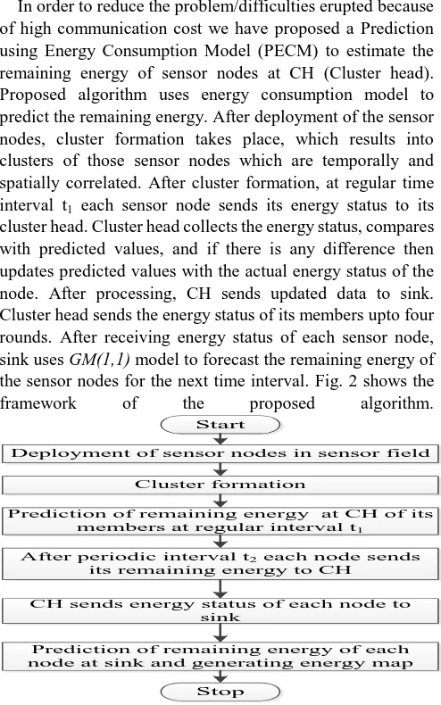
In order to reduce the problem/difficulties erupted because of high communication cost we have proposed a Prediction using Energy Consumption Model (PECM) to estimate the remaining energy of sensor nodes at CH (Cluster head). Proposed algorithm uses energy consumption model to predict the remaining energy. After deployment of the sensor nodes, cluster formation takes place, which results into clusters of those sensor nodes which are temporally and spatially correlated. After cluster formation, at regular time interval t1 each sensor node sends its energy status to its cluster head. Cluster head collects the energy status, compares with predicted values, and if there is any difference then updates predicted values with the actual energy status of the node. After processing, CH sends updated data to sink. Cluster head sends the energy status of its members upto four rounds. After receiving energy status of each sensor node, sink uses GM(1,1) model to forecast the remaining energy of the sensor nodes for the next time interval. Fig. 2 shows the

framework of the proposed algorithm.

Cluster formation

Prediction of remaining energy at CH of its

members at regular interval t1

CH sends energy status of each node to sink

Deployment of sensor nodes in sensor field

After periodic interval t2 each node sends

its remaining energy to CH

Prediction of remaining energy of each node at sink and generating energy map

Start

Stop

Fig. 2.Framework of proposed prediction algorithm. An adaptive clustering protocol for wireless sensor networks is used in cluster formation [17]. Initially to exploit spatial correlation, given sensor field is divided into virtual grids. Temporal correlation is exploited using data mining techniques among sensor nodes

International Journal of Innovative Technology and Exploring Engineering (IJITEE) ISSN: 2278-3075, Volume-8 Issue-12, October 2019

cluster head gathers data from its members and generates frequent itemsets exploiting temporal correlation among its members. These frequent itemsets are further processed by sink to form temporally and spatially cohesive clusters. Grey model is used to forecast the upcoming values of a time series based upon current history. The first assumption of grey model is that only positive data values are to be used. The second assumption is that the sampling frequency of series is fixed. Further GM (1,1) is widely used in prediction because of its computational efficiency. GM (1,1) is used to obtain future values from current values of sensor node. The predictions using grey model are based on past data values. Initially these data values are stored to build the initial data

sequence for GM (1,1) model. It is denoted as

Where is a non-negative sequence of remaining energy of the sensor node and n is the size of the sample. After that

Accumulation Generation Operator (AGO) is used on to

obtain the series .

Where

The generated mean sequences of is defined as:

Here is the mean value of adjacent data defined in following equation.

And the projected value of information at time k + H is given by following equation:

In a given cluster, each sensor node can be in one of the two

states: either it is serving as cluster head (CH) or it is a

member of the cluster. While acting as cluster head, the node

has to receive and transmit data on behalf of its members also.

For a given sensor node si, let the probability of being a cluster

head is and probability of being a member of the

cluster is

.

while transmitting data, receiving data and data processing.

Although while a node is idle then least amount of energy is

consumed. Energy consumption also depends upon the

amount of data transmitted/received/processed. Thus, the

energy consumed by the node si can be expressed as following

equation.

Where

,

time t, is the data received up to time t, is the

data transmitted up to time

t,

to time t, is the energy consumed in processing per unit

data, is the energy consumed per unit time while

idle mode and is time period up time t, for which

node si remains idle. When sensor node si act as a cluster head

then the energy consumed up to time t is given by following

equation.

Thus, the overall energy consumed by a node si up to time t is

given by following equation.

remaining energy, at time t can be computed by following equation.

Where is energy at time t = 0, i.e. initial energy of node si.

Fig. 3.Working at CH.

After fourth round, each sensor node waits for broadcast message about average difference from sink. After receiving AD information, each sensor node computes difference between its current remaining energy level and last communicated remaining energy level. If computed difference and AD received from sink is within defined limit then no action has been taken, otherwise actual value of current remaining energy level is communicated to sink through respective CH. After receiving such values, sink will update the respective queue entry by actual received value. It will help to reduce the error in prediction.

IV. SIMULATIONOFPROPOSEDALGORITHM

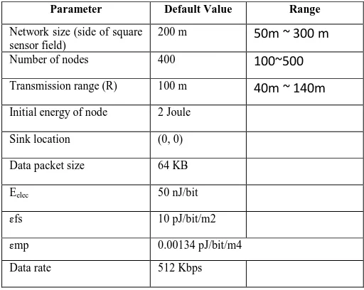
In this section, performance evaluation of the of proposed algorithm by simulating it in MATLAB is performed. Simulation parameters along with performance matrices Number of Messages and Network Lifetime (First Node Die (FND) and Half Node Die (HND)) are used. The effect of number of nodes on performance metrics to measure the effectiveness of proposed algorithm is also studied. To analyses the performance, proposed protocol is compared with existing approaches TinyDB [19] and INLR[9]. TinyDB is the foremost work pointing the application of contour mapping. In its one of the versions where aggregation is not performed, all nodes are required to send their values. In TinyDB, in-network computations are directly proportional to number of nodes. INLR requires values from each sensor node to create contour map. INLR also uses model based partial map aggregation which helps in reducing overheads. Simulation parameters are listed in Table 1.

Fig. 4.Working at Sink. Table 1: Simulation Parameters

Parameter Default Value Range

Network size (side of square sensor field)

200 m _{50m ~ 300 m}

Number of nodes 400 _100~500

Transmission range (R) 100 m _{40m ~ 140m}

Initial energy of node 2 Joule

Sink location (0, 0)

Data packet size 64 KB

Eelec 50 nJ/bit

ɛfs 10 pJ/bit/m2

ɛmp 0.00134 pJ/bit/m4

Data rate 512 Kbps

International Journal of Innovative Technology and Exploring Engineering (IJITEE) ISSN: 2278-3075, Volume-8 Issue-12, October 2019

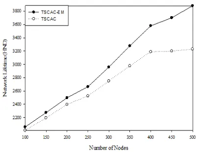
Fig. 5.Effect of number of nodes on number of messages Proposed algorithm inherits clustering mechanism from previously proposed Temporal-Spatial Correlation based Adaptive Clustering algorithm TSCAC [17]. Simulation results have been compared among TSCAC and TSCAC with proposed algorithm (TSCAC-EM). Fig. 6 and Fig. 7 show the comparison of network lifetime and number of sensor nodes. Fig. 6 shows the number of rounds spent till the first node in the deployed network dies and Fig. 7 shows the number of rounds spent until fifty percent of nodes in the deployed network die.

Fig. 6.Effect of number of nodes on FND

To analyze the result of the quantity of nodes on the network lifetime, transmission range is kept 100 m and the network size is kept 200m x 200m. It can be realized from the graph, network lifetime increases both in terms of First Node Die and Half Node Die with escalation in the number of nodes. When the node density is less, a smaller number of nodes will go to sleep mode or in other words more percentage of nodes will be active and hence they all consume energy and the chance of occurrence of (FND) and (HND) will take place at lesser number of rounds. With the increase in node density, though the overall network energy consumption increases but the burden on the nodes will be shared as a result of which energy consumption per node will be reduced and hence nodes can survive for a greater number of rounds.

Fig. 7.Effect of number of nodes on HND

In case of TSCAC-EM network life time improves as compare to TSCAC, because TSCAC-EM balance the energy consumption by monitoring the remaining energy of each part of the network through cluster head.

V. CONCLUSION

Energy maps can be utilized for extending the lifetime of network. In the proposed research, by utilizing the grey system theory-based prediction is used to predict the residual energy. Predicted energy status is used for creating energy map in order to extend the network lifetime. In the proposed algorithm, the sink node predicts the remaining energy of the nodes based upon the collected remaining energy information. Simulation results prove the usefulness of the proposed algorithm. Proposed algorithm inherits our previously proposed clustering algorithm (TSCAC). The network lifetime of TSCAC-EM (TSCAC with Energy Map) marginally improves over the TSCAC. The major contribution of the proposed energy map algorithm is to identify the critical regions, where the energy depletion rate is high. Thus, node replacement policy can be framed or load can be balanced among other nodes to avoid network partitioning.

ACKNOWLEDGMENT

REFERENCES

1. K. Romer and F. Mattern, “The Design Space of Wireless Sensor Networks,” IEEE Wirel. Commun., vol. 11, no. 6, pp. 54–61, 2004 2. V. Katiyar, N. Chand, and N. Chauhan, “Recent advances and future

trends in Wireless Sensor Networks,” vol. 1, no. 3, pp. 330–342, 2010. 3. T. Haenselmann, “Sensor Networks,” 2009.

4. I. F. Akyildiz, W. Su, Y. Sankarasubramaniam, and E. Cayirci, “Wireless Sensor Networks: A Survey,” Comput. Networks, vol. 38, no. 4, pp. 393–422, 2002.

5. V. Katiyar, N. Chand, and S. Soni, “Grey System Theory-Based Energy Map Construction,” pp. 122–131, 2011.

6. J. Zhao, R. Govindan, and D. Estrin, “Residual Energy Scans for Monitoring Wireless Sensor Networks,” in Proceedings of the IEEE Wireless Communications and Networking Conference, 2002, pp. 356–362.

7. E. Chan and S. Han, “Energy Efficient Residual Energy Monitoring in Wireless Sensor Networks,” Int. J. Distrib. Sens. Networks, vol. 5, no. 6, pp. 748–770, 2009.

8. B. Deb, S. Bhatnagar, and B. Nath, “A Topology Discovery Algorithm for Sensor Networks with Applications to Network Management,” 2001. 9. M. Li and Y. Liu, “Iso-Map:

Trans. Knowl. Data Eng., vol. 22, no. 5, pp. 699–710, 2010.

10. R. A. F. Mini, M. Do Val Machado, A. A. F. Loureiro, and B. Nath, “Prediction-based energy map for wireless sensor networks,” Ad Hoc Networks, vol. 3, no. 2, pp. 235–253, 2005.

11. J. N. Al-karaki, G. A. Al-Mashaqbeh, and G. A. Al-mashagbeh, “Energy-Centric Routing in Wireless Sensor Networks,” Microprocess. Microsyst., vol. 31, no. 4, pp. 252–262, 2007.

12. R. A. F. Mini, A. A. F. Loureiro, and B. Nath, “The Distinctive Design Characteristic of A Wireless Sensor Network : The Energy Map,” Comput. Commun., vol. 27, no. 10, pp. 935–945, 2004.

13. M. N. Halgamuge, M. Zukerman, and K. Ramamohanarao,“An Estimation Of Sensor Energy Consumption,” vol. 12, pp. 259–295, 2009.

14. A. Kumar, N. Chand, and V. Kumar, “Location Based Clustering in Wireless Sensor Networks,” in World Academy of Science, Engineering and Technology, 2011, pp. 1977–1984.

15. W. B. Heinzelman, A. P. Chandrakasan, and H. Balakrishnan, “An Application-Specific Protocol Architecture for Wireless Microsensor Networks,” IEEE Trans. Wirel. Commun., vol. 1, no. 4, pp. 660–670, 2002.

16. I. Rekleitis, D. Meger, and G. Dudek, “Simultaneous Planning, Localization, and Mapping in a Camera Sensor Network,” Rob. Auton. Syst., vol. 54, pp. 921–932, 2006.

17. R. Kumar, N. Chauhan, and N. Chand, “Adaptive Clustering in Wireless Sensor Networks,” International Journal of Multimedia and Ubiquitous Engineering, Vol.12, No.9, pp.15-26, 2017.

18. D. Julong, “Introduction to Grey System Theory,” J. Grey Syst., vol. 1, pp. 1–24, 1988.

19. W. Xue, Q. Luo, L. Chen, and Y. Liu, “Contour Map Matching for Event Detection in Sensor Networks,” SIGMOD Int. Conf. Manag. Data, pp. 145–156, 2006.

AUTHORSPROFILE

Rajeev Kumar received his BTech. degree from National Institute of Technology Surathkal, Karnatka and MTech degree from and National Institute of Technology Hamirpur (INDIA). Currently he is pursuing his PhD from National Institute of Technology, Hamirpur. His research interest includes Graph Theory, Computer Security, Adhoc Networks, and Wireless Sensor Networks.

Naveen Chauhan joined NIT Hamirpur as Associate, prior to this he has served as Assistant Professor. He has received his Ph.D. (Computer Science & Engineering) from NIT Hamirpur in 2012. His research interest includes Mobile Wireless Networks with special emphasis towards Mobile Ad hoc Networks, Sensor Networks, Vehicular Ad hoc Networks, Internet of Things, Internet of Vehicles and their Security aspects. Naveen Chauhan has excellent research contributions in these areas and has published research articles in large number of Journals (including SCI and Scopus indexed Journals).