Calculation on Yield Strain Depending on Time of Corrosion Influence

International Journal of Innovative Technology and Exploring Engineering (IJITEE) ISSN: 2278-3075, Volume-8 Issue-7, May, 2019



Abstract: In the design of steel structures, the main value of the steel elements in the yield strain point is taken into account in the calculations. Over time, corrosion occurs on steel structures, indicating a negative influence. When a steel element is subjected to corrosion in a particular corrosion category, its mechanical properties change. Although there are many studies in the field of change, there is no uniform formula or equation that can be used to calculate the possible change in the value on yield strain. This fact prevents the preliminary assessment that can be made as regards the possibility of continued use of the corroded steel element. The processing of experimental data is a cumulative process as different data are obtained from each test. Still a non-essential single equation or formula that has sufficient practical accuracy, it is possible to determine the influence of corrosion on a steel element in a future form. There are two basic ways that can be grouped - the original state is well known, then the future state can theoretically be predicted so-called deterministic process or this is a process that is a set of random variables - a stochastic process. I conducted a survey, collected and analyzed the available database regarding the change of values in the yield strain point. I processed values using the stochastic way and the average method. From this data processing I have compiled diagrams that show the change in values over time. I used the polynomial approximation and found the equation where the values change. I have come to the conclusion that the proposed equations are sufficiently precise and can be used in practice.

Index Terms: yield strain, calculation, corrosion, influence, time.

I. INTRODUCTION

The problem of corrosion in steel building elements and structures (Fig.1) is a complex task [1-3, 9, 11-20]. The anticorrosive protection of steel structures and elements is a made-up task. Anticorrosive protection measures - lacquer coatings and systems [1-3] have been developed under operating conditions, which, however, significantly increases the operational costs, and their construction reliability is reduced as the number of coatings increased over time. Given the dependence as well as the specific factors of the elements, such as the probability of corrosion and fracture irregularities in the cross-sectional perimeter of the elements, it is not possible to establish the dependence of the bearing capacity of the metal structures during operation, especially needed in the reconstruction of the structural component structures and the assessment of the suitability of the structures for further exploitation. We should look for ways to predict the corrosive impact, which has a negative impact on the main features - reduction of geometric characteristics, appearance

Revised Manuscript Received on May 06, 2019

Antonio Shopov, Department “Strength of materials”, Technical University of Sofia, 8, “KlimentOhridski” blvd., Sofia, Bulgaria.

of surface defects, structural changes in the material and strength-deformation properties of steel, which also affects the parameters of the technical equipment and systems [11-20]. Some authors offer a variety of dependencies to determine the influence of corrosion on mechanical properties [9, 11-20], but there are no equations that summarizes the experimental results and to be easy used by engineers in practice.

Experimental data for the investigation of metal constructions and elements operated at aggressive corrosive environment and after treatment should be correlated with the effect of corrosion on values on yield strain, describing with a polynomial function.

Fig. 1. Structure with corroded steel elements

II. METHOD

In mathematics, the approximation theory deals with how best to approximate functions with simpler functions and quantify their mistakes [4,5]. Recognizing that what is best and simpler will depend on the application [4]. Closely related is the topic of function approximation through generalized Fourier series, i.e. approximations based on the summation of a series of terms based on orthogonal polynomials [4, 5]. One of the problems of particular interest is the approximation of a function using operations in order for the approximation to be as close as possible to the actual function, usually with an accuracy close to that of the floating-point arithmetic of the basic parameter [4, 5]. This is achieved by using a high degree and / or narrowing polynomial over which the polynomial must approach the function [4, 5]. Polynomials are functions with useful properties [4, 5]. Their relatively simple form makes them ideal for use as approximations for more complex functions [4]. The polynomial in f (x) is a function of the form [4] (eq. 1):

(1)

Calculation on Yield Strain Depending on Time

of Corrosion Influence

If we look at cases in which, instead of knowing function expression, we have point values [4]. It is enough to find a polynomial that passes through these points, and we want the polynomial to pass through the given data, i.e. interpolating polynomial [5]. Let us assume that we know (or choose to try) the function f (x) exactly at several points and that we want to approximate the behavior of the function between these points [4]. In its simplest form, this is equivalent to linear assembly (Fig. 2 (a)), but it is often more accurate to look for a curve that has no "angles" in it (Fig. 2 (b)) [4].

(a) (b)

Fig. 2. (a) Linear connection of the dot-to-dot principle [4]; (b) dot-to-dot connection by function (no "angles") [4]

In case we have experimental data after an experiment and after making a line (function), passing as close as possible to the data that is obtained [4, 5].

III. ESTABLISHINGDEPENDENCIES There are many studies with experimental data presented, the change of certain indicators from mechanical properties due to the corrosive impact [9, 11-20]. These data are processed in the stochastic way and average method and the results are make a graphics. Using the polynomial approximation [4, 5, 11], I found the equation of change the value on yield strain is determined in dependence on the time of corrosion. For each corrosion category. After I processed experimental data with stochastic way [6-8, 10] and average method, I make up a graphics on dependence on yield strain in time of corrosion influence i.e. εy (t) where t is a time in months on corrosion

impact according a corrosion category.

A. Corrosion category C1

On Fig. 3 shows the dependence between the change of the yield strain and the time of influence of the corrosion category.

From Fig. 3, using the polynomial approximation [4, 5, 11], a functional dependence for the change of yield strain and the time of impact of the corrosion category (in months) is established depending on the chosen method of data processing (eq. 2 and eq. 3).

On Table I is present a result after processing by stochastic method and average method.

TABLE I RESULTS AFTER PROCESSING

time, [months]

Yield Strain, [%]

stochastic method average method

0 0.200000 0.200000

9138 0.225067 0.226024

14769 0.240820 0.232762

24923 0.232340 0.236824

34892 0.218667 0.181215

46154 0.248667 0.223234

54000 0.218493 0.215416

64615 0.184587 0.169523

73108 0.124187 0.115477

77262 0.112800 0.113920

Fig. 3. Graphics on dependence on yield strain in time of corrosion influence -corrosion category C1.

 Stochastic results:

(2)

 Average results:

₍₃₎

B. Corrosion category C2

On Table II is present a result after processing by stochastic method and average method.

On Fig. 4 shows the dependence between the change of the yield strain and the time of influence of the corrosion category.

International Journal of Innovative Technology and Exploring Engineering (IJITEE) ISSN: 2278-3075, Volume-8 Issue-7, May, 2019

TABLE II RESULTS AFTER PROCESSING

time, [months]

Yield Strain, [%]

stochastic method average method

0 0.200000 0.200000

475 0.225067 0.226024

768 0.240820 0.232762

1296 0.232340 0.236824

1814 0.218667 0.181215

2400 0.248667 0.223234

2808 0.218493 0.215416

3360 0.184587 0.169523

3802 0.124187 0.115477

4018 0.112800 0.113920

Fig. 4. Graphics on dependence on yield strain in time of corrosion influence -corrosion category C2.

 Stochastic results:

(4)

 Average results:

(5)

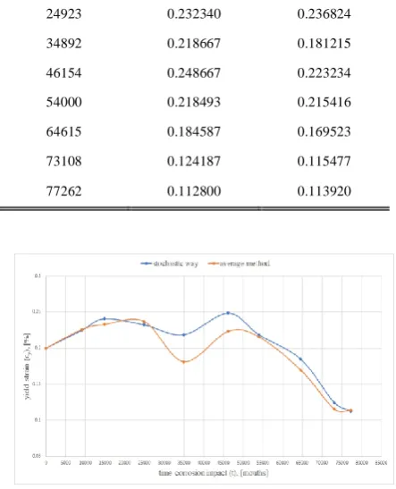
C. Corrosion category C3

On Fig. 5 shows the dependence between the change of the yield strain and the time of influence of the corrosion category.

On Table III is present a result after processing by stochastic method and average method.

TABLE III RESULTS AFTER PROCESSING

time, [months]

Yield Strain, [%]

stochastic method average method

0 0.200000 0.200000

238 0.225067 0.226024

384 0.240820 0.232762

648 0.232340 0.236824

907 0.218667 0.181215

1200 0.248667 0.223234

1404 0.218493 0.215416

1680 0.184587 0.169523

1901 0.124187 0.115477

2009 0.112800 0.113920

Fig. 5. Graphics on dependence on yield strain in time of corrosion influence -corrosion category C3.

From Fig. 5, using the polynomial approximation [4, 5, 11], a functional dependence for the change of yield strain and the time of impact of the corrosion category (in months) is established depending on the chosen method of data processing (eq. 6 and eq. 7).

 Stochastic results:

(6)  Average results:

₍₇₎

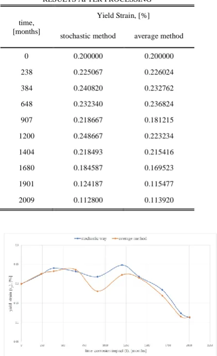
D. Corrosion category C4

On Table IV is present a result after processing by stochastic method and average method.

TABLE IV RESULTS AFTER PROCESSING

time, [months]

Yield Strain, [%]

stochastic method average method

0 0.200000 0.200000

149 0.225067 0.226024

240 0.240820 0.232762

405 0.232340 0.236824

567 0.218667 0.181215

750 0.248667 0.223234

878 0.218493 0.215416

1050 0.184587 0.169523

1188 0.124187 0.115477

1256 0.112800 0.113920

On Fig. 6 shows the dependence between the change of the yield strain and the time of influence of the corrosion category.

From Fig. 6, using the polynomial approximation [4, 5, 11], a functional dependence for the change of yield strain and the time of impact of the corrosion category (in months) is established depending on the chosen method of data processing (eq. 8 and eq. 9).

Fig. 6. Graphics on dependence on yield strain in time of corrosion influence -corrosion category C4.

 Stochastic results:

(8)  Average results:

(9)

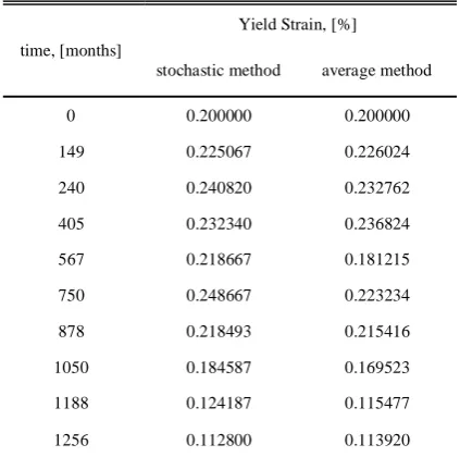
E. Corrosion category C5

On Table V is present a result after processing by stochastic method and average method.

TABLE V RESULTS AFTER PROCESSING

time, [months]

Yield Strain, [%]

stochastic method average method

0 0.200000 0.200000

59 0.225067 0.226024

96 0.240820 0.232762

162 0.232340 0.236824

227 0.218667 0.181215

300 0.248667 0.223234

351 0.218493 0.215416

420 0.184587 0.169523

475 0.124187 0.115477

502 0.112800 0.113920

On Fig. 7 shows the dependence between the change of the yield strain and the time of influence of the corrosion category.From Fig. 7, using the polynomial approximation [4, 5, 11], a functional dependence for the change of yield strain and the time of impact of the corrosion category (in months) is established depending on the chosen method of data processing (eq. 10 and eq. 11).

Fig. 7. Graphics on dependence on yield strain in time of corrosion influence -corrosion category C5.

International Journal of Innovative Technology and Exploring Engineering (IJITEE) ISSN: 2278-3075, Volume-8 Issue-7, May, 2019

(10)

 Average results:

(11)

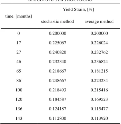
F. Corrosion category CX

On Table VI is present a result after processing by stochastic method and average method.

TABLE VI RESULTS AFTER PROCESSING

time, [months]

Yield Strain, [%]

stochastic method average method

0 0.200000 0.200000

17 0.225067 0.226024

27 0.240820 0.232762

46 0.232340 0.236824

65 0.218667 0.181215

86 0.248667 0.223234

100 0.218493 0.215416

120 0.184587 0.169523

136 0.124187 0.115477

143 0.112800 0.113920

On Fig. 8 shows the dependence between the change of the yield strain and the time of influence of the corrosion category

Fig. 8. Graphics on dependence on yield strain in time of corrosion influence -corrosion category CX.

From Fig. 8, using the polynomial approximation [4, 5, 11], a functional dependence for the change of yield strain and the time of impact of the corrosion category (in months) is established depending on the chosen method of data processing (eq. 12 and eq. 13).

 Stochastic results:

(12)

 Average results:

(13)

Probability of results – stochastic results is 82.72 % and average results is 71.54 % for steel S355JR.

If I remove values from the formulas, I establish with sufficient practical accuracy, a basic non-liner equation (eq. 14):

(14)

Where: А1, А2, А3, А4, А5, А6, А7, А8 и А9 is constant

values and need to be determined experimentally in every case.

IV. DISCUSION

V. CONCLUSION

Yield strain begins to decrease depending on the development of corrosion, which means there is a correlation between corrosion and yield strain.

After careful analysis of the established graphs and values, the co-existence is determined on values of yield strain, whose co-determination depends solely on the rate of corrosion on the steel elements.

The established formula has its practical significance and provides an opportunity for a preliminary calculation of the expected change in yield strain under the corresponding corrosion impact. The formula is a special case, it can be used in practice, especially to establish possibilities for re-use of a corroded steel element.

It is well known that steel is a ductile material, which, as a result of its corrosive action, becomes brittle. This is also confirmed by the formulas given. It should be sought to take into account the fact that corrosion reduces cross-section, which directly affects load-bearing capacity.

The determination of the corrosion rate in steel elements should not be ignored and should be taken into account in order to assess the point where this corrosion element would not be usable.

ACKNOWLEDGMENT

This research was supported by “Hyosel” Ltd., Sofia, Bulgaria.

The author would like to thank for the support on BorislavBonev,Technical University of Sofia, Faculty of Electronic Engineering and Technologies, Department „Microelectronics

REFERENCES

1. Z. Ahmad. Principles of corrosion engineering and corrosion control. Elsevier, 2006. ISBN: 9780750659246

2. M. Kulicki, Z. Prucz, D. Sorgenfre and D. Mertz. Guidelines for evaluating corrosion effects in existing steel bridges. 1990.

ISBN 0309048567

3. P. Marcus. Corrosion mechanisms in theory and practice. CRC press, 2011. ISBN 9781138073630

4. L. Trefethen. Approximation theory and approximation practice. Siam, 2013. ISBN: 9781611972399

5. M. Powell. Approximation theory and methods. Cambridge university press, 1981. ISBN: 0521295149

6. L. Evans. An introduction to stochastic differential equations. American Mathematical Soc., 2012. ISBN: 9781470410544 7. F. Klebaner. Introduction to stochastic calculus with applications.

World Scientific Publishing Company, 2012. ISBN: 9781860945663 8. D. Arseniev, V. Ivanov and M. Korenevsky. Adaptive Stochastic

Methods: In Computational Mathematics and Mechanics. Walter de Gruyter GmbH & Co KG, 2018. ISBN: 9783110489644

9. A. Shopov and R. Ganev. Survey on the multi-annual influence of atmospheric conditions on the strain of the reinforced steel Ф6,5 (A-I) for reuse. Annual of UACEG, 51.10, 2018, pp. 21-28. in Bulgarian. 10. A. Shopov. Stochastic way for calculation of strength on construction

steel with corrosion. In: XVIII Anniversary International Scientific Conference by Construction and Architecture “VSU’2018“, Sofia, Bulgaria, 2018, 1.1: pp.413-418.in Bulgarian.

11. A. Shopov and B. Bonev. Change of young’s module on steel specimens with corrosion by experiment. International Journal of Modeling and Optimization, 9.2, 2019, pp.102-107.

12. A. Shopov and B. Bonev. Ascertainment of the change of the ductility in corroded steel specimens by experiment. International Journal of Civil Engineering and Technology, 10.1, 2019, pp. 1551-1560. 13. A. Shopov and B. Bonev. Experimental study of the change of the

strengthening zone on corroded steel specimens. International Journal of Civil Engineering and Technology 10.1, 2019, pp. 2285-2293.

14. A. Shopov and B. Bonev. Experimental determination on the change of geometrical characteristics and the theoretical ultimate-load capacity of corroded steel samples. International Journal of Civil Engineering and Technology 10.2, 2019, pp.320-329.

15. A. Shopov and B. Bonev. Study by experimental of the zone of fracture on S355JR steel specimens with corrosion. International Journal of Civil Engineering and Technology, 10.2, 2019, pp.751-760.

16. A. Shopov and B. Bonev. Experimental study of zone of yield strength on corroded construction steel specimens for reuse. In: MATEC Web of Conferences 279. EDP Sciences, 2019. p. 02009.

17. Chen Jia, Y Shao, L Guo and Y Liu. Incipient corrosion behavior and mechanical properties of low-alloy steel in simulated industrial atmosphere. Construction and Building Materials, 2018, 187: pp.1242-1252.

18. F. Xu, Y. Chen, X. Zheng, R. Ma and H. Tian. Experimental Study on Corrosion and Mechanical Behavior of Main Cable Wires Considering the Effect of Strain. Materials, 2019, 12.5: 753

19. K. Mohammad, C. Adam and A. Nicholas. Stress-Strain Response of Corroded Reinforcing Bars under Monotonic and Cyclic Loading. 15 WCEE, Lisboa, 2012.

20. G. Chen, H. Muhammad, G. Danying and Z. Liangping. Experimental study on the properties of corroded steel fibres. Construction and Building Materials, 2015, 79: pp.165-172.

AUTHORPROFILE