Comparative Analysis Of Different Imputation Techniques For Handling Missing Dataset

International Journal of Innovative Technology and Exploring Engineering (IJITEE) ISSN: 2278-3075, Volume-8 Issue-7, May, 2019



Abstract: In last two decades data became the wealth because of its importance in different fields. But it’s very difficult to collect all the information and store it as data in real time which results in some missing data. Missing data cannot be omitted because even small piece of data plays a major role in the output. Imputation plays a major role in handling missing data before we predict the hidden patterns in it. In this paper our aim is to, discuss about different techniques to handle missing data, together with some relatively simple approaches that can often yield reasonable results. However our aim is to replace the missing values by the predicted values with the help of eight different imputation algorithms and we will conclude with the best algorithm.

Index Terms: Handling incomplete data, Imputation, Imputation techniques and Missing data.

I. INTRODUCTION

Firstly, how the missing data can occur explains in paper [1],[4], there are many reasons: equipment and data recording or collecting may malfunction, there are chances for the participants failed response to question either legitimately or illegitimately, subjects can withdraw from studies before they are completed, and data entry errors can occur, and the elimination of extreme scores and outliers can also be the cause of missingness.

Figure 1 Layout of the process.

In figure 1, the general work flow was showed diagrammatically. The incomplete data from the database was taken a treated with different imputation methods to make it complete dataset which will obviously give best results. The issue with missingness is that nearly all techniques assume to have complete data and most common procedures default to have least desirable options for dealing with missing data: deletion of the case from the analysis, was

Revised Manuscript Received on April 06, 2019.

Durgaprasad N, Computer science and engineering, Karunya institute of technology and sciences, Coimbatore, India.

Gopal Krishna M, Computer science and engineering, Karunya institute of technology and sciences, Coimbatore, India.

Deepa Kanmani S, Computer science and engineering, Karunya institute of technology and sciences, Coimbatore, India.

Sravan Reddy G, Computer science and engineering, Karunya institute of technology and sciences, Coimbatore, India.

Revanth Reddy D, Computer science and engineering, Karunya institute of technology and sciences, Coimbatore, India.

in paper [5]. Most people allow the software to default elimination of important data from their analysis of quantitative data, despite the individual or case potentially having a good deal of other data to contribute to the overall analysis. Three general types of missing values:

1) Missing Completely At Random (MCAR): When missing data belongs to this type, the missing data is completely independent of the other variables and parameters of interest. In this case, the analysis performed on the data is unbiased.

2) Missing At Random (MAR): In MAR, the data is missing at a certain rate but that rate depends on some other variable on the data. When there are many missing values in a certain category then this type of data can induce a bias when analyses.

3) Missing Not At Random (MNAR): In this case, the missingness of a certain value depends on the true value itself. Imputation is the process of interchanging missing data with substituted values. In paper [6], the author has given the introduction of imputation like this, to impute any value in the place of missing value we cannot simply substitute some random value, first of all, we need to estimate a value according to the data available and then substitution process should go on. Now the problem is how to estimate value from the data available, here come the different imputation methods to handle missing data. Mainly, there are two types of imputation techniques. One is single imputation and the other type is multiple imputations. Many of the cases multiple imputation methods are highly recommended over single imputation for achieving good accuracy.

II. RELATED WORKS

In paper [2], author discussed the ways of handling missing data. According to them the missing data presence in data will affect its performance and will not be good for predictions. Different methods are there to handle missing data but mainly two different methods they mentioned is Deletion and Imputation. Discarding the instances with missing data by Case Deletion is not a good idea because every single piece of data is having its own importance in the data prediction. So practically Imputation plays a major role in handling missing data. This may be achieved through either single imputation or multiple imputation. In this paper author used single imputation methods to handle missing data like Mean, Median,

KNN imputation procedure.

Comparative Analysis Of Different Imputation

Techniques For Handling Missing Dataset

Multiple Imputation methods are discussed in paper [3]. They have stated a way to handle missing data with the help of Random Forest Imputation to predict the missing data. So our aim is to use the same methods to solve the missingness problem and to impute the missing data.

III. EXPERIMENTAL ANALYSIS

A. Missing Dataset and Patterns

For our analysis purpose heart disease dataset with 14 variables each with 302 observations is chosen. The missingness of the dataset is analyzed with the help of some MICE and Naniar functions. Naniar function vs_miss() is used in order to know the missing pattern of the dataset and visual representation of the data pattern is here.

Figure 2 Visual representation of the percentage of data.

As Figure 2, shows different variables which have different amounts of missing data in it. The image also explains that there is 40% of missing data in this dataset where 60% is present. But in real-time scenarios the amount of missing data varies, so in order to address this problem different datasets with different amount of missing data is taken into count and are imputed with the following techniques.

B. Mean

Mean imputation is one of the simple technique for handling missing data. The missing value on a variable is replaced by the mean value of the available data of that particular variable [4]. It is easy to use, but the inconsistency in the data will be reduced, therefore the standard deviations and variance estimates tend to be miscalculated. By restricting the variability the magnitude of the covariance and correlation decreases and it causes bias. In conclusion to MEAN, it is clear that there are many disadvantages than advantages of mean imputation. The advanced imputation methods can be preferred instead of mean, such as predictive mean matching (PMM) etc.

C. Median

Whenever we talk about simple imputation techniques we immediately think of median after mean. In paper [6], they have explained about median like this, the median is the process in which the middle value of all the values in a variable is used to substitute in the place of missing data. The advantages and disadvantages are almost the same in both mean and median imputation.

D. K-Nearest Neighbors (KNN)

This algorithm works based on matching a point with its closest k neighbors in a multi-dimensional space. It is useful

for dealing almost all kinds of missing data such as continuous, discrete, ordinal and categorical. In paper [8], the KNN working was described, by using KNN for missing values the value of the point can be guessed from the values of the points nearest to it. There are so many parameters that should take into consideration when we are using the KNN algorithm. The number of neighbors to look for. K refers to the number of neighbors, let's say, if we consider a low k then the influence of noise will get increased and the results are going to be less generalizable. In contrast, when we consider high k then the local effects tend to blur and that's what we are actually looking for. Taking odd k is highly recommended for binary classes to avoid ties. Arithmetic mean, median and mode for numeric variables and mode for categorical ones can be used for aggregating.

Normalization of data is necessary especially when we calculate compute the Euclidean distances between points. For instance, there is a 2D plot which contains weight (lb) on the Y-axis and height (cm) on the X-axis. When we calculate the Euclidean distance between 2 points in the plot with the same scale of lb and cm then the result would be inconsistent, so by normalizing the scale would be same and the results can be considerable and comparable. There are many types of normalizations like Z-score, Max-Min etc. Euclidean and Manhattan are the main ones among several distance metrics which are available. Using Euclidean is the best in the case of similar input variables. Manhattan method is good if the input variables are not similar in type.

E. Linear regression

In this model, our aim is to establish a regression line depending on the relationship between dependent and independent variables. This regression line can be represented by a linear equation according to paper [9].

(1) In equation 1, each variable was described as follows. Y – Dependent Variable, a – Slope, X – Independent variable, b – Intercept.

These quantities ‘a’ and ‘b’ are derived based on minimizing the sum of squared difference of distance between data points and regression line. There are two types of imputations in this model.

1. Simple Linear Regression: It is regarded as single independent variable. Suppose there is a numeric variable with missing data. For instance, the variable Y is a numeric variable that contains 3 missing values and our goal is to do is to identify the most correlated variable present in the dataset with Y and then fit a regression model of Y on that variable and predict for the missing values. 2. Multiple Linear Regression: Multiple Linear

International Journal of Innovative Technology and Exploring Engineering (IJITEE) ISSN: 2278-3075, Volume-8 Issue-7, May, 2019

(2) The equation 2 represents the sample multiple regression model of Y. Here both X and Z are independent variables.

F. MICE

MICE which is known as Multiple Imputation by Chained Equations helps to impute missing data with acceptable values. This was explained by paper [11]. These values are specially designed based on and for each missing point. MICE is one of the multiple imputation techniques which assumes the missing data is MAR category which takes only observed values into a count. MICE is mainly developed to handle the large datasets with thousands of rows and hundreds of variables with different types of data and each of those data types will be handled with different models. Steps to handle missing data is as given below.

Step 1. At first, all the missing data is imputed with the help of the mean values of the column values.

Step 2. The mean values are stored as "place holder" and these values are set back to miss.

Step 3. The values of step 2 are stored in the variable the named var.

Step 4. These values in variable var are used to regress the other values in the dataset.

Step 5. All these models work the same when we try to execute in the same process outside the MICE.

The observed and imputed values will combined to form the complete dataset with the help of chained reactions. We can generate any number of imputed datasets with the help of chained reactions and recent studies state that 5-10 sets are sufficient to handle the missing data very efficiently.

G. Random Forest

In paper [11], the random forest will consider two datasets. Firstly, missing data in the original dataset used to create the random forest and another type is missing data in a new sample that we want to categorize. The general idea for missing data in any context is to make an initial guess that could be bad and then gradually refine the guess until it is hopefully a good guess. The bad guess for the numeric variable is substituting the missing value with the median value from values of that variable. If the variable values are YES or NO type then the bad guess would be the most number of occurrence one either it is YES or NO. Now the incomplete dataset becomes a complete one. Now we want to refine the guesses. We do this by first determining which samples are similar to the one with missing data. Now there are some steps to find the similarity.

Step 1: Build a Random forest that means to build the decision trees with the data in the dataset.

Step 2: Run all of the data down all of the trees.

Firstly, start by running all of the data down the first tree. Identify that if any two or more samples ended up at the same leaf node that means they are similar. This is how similarity has to find in a random forest. One can keep track of similar samples using the proximity matrix. The proximity matrix has a row and a column for each sample. Mark 1 at the positions where the similarity for the first tree has found and increment the count while checking for the rest of the trees. Finally, the proximity matrix with the values get filled then divide each value with the number of trees considered. These proximity values can be used for the samples having missing data to make better guesses about missing data. If the variable

is YES or NO type then we calculate the weighted frequency of YES and NO using proximity values as the weights. After calculating the weighted frequency of both YES and NO then compare both the values. If weighted frequency for YES is greater, then the value “YES” has the high probability to become correct substitution in the corresponding position of missing data and the same in the case of NO.

H. Predictive Mean Matching

Predictive Mean Matching (PMM) is a smart way to do imputation of missing values, especially when monotonic patterns in missingness has existed in the beginning stages of the invention of PMM. But now anyway PMM is included in almost all the software packages that implement multiple imputations. PMM produces imputed values that almost fits like real values. If the original values are skewed then imputed values are also skewed as in paper [10].

The process of PMM and its working procedure was explained in the following six steps. Let assume that there is a variable named A, with some missing data, and the group of variables B with no missing data in them which helps to impute A. Then do the following steps.

Step 1. Estimate the linear regression model where the model will be estimated by existed values of both A and B. Step 2. Aimlessly draw a posterior predictive distribution of C to produce a new set of coefficients C∗ which is a multivariate distribution of mean C and covariance matrix of C.

Step 3. With the help of C predict values for existed and missing places of A.

Step 4. For each case where A is missing, find the neighboring predicted values among the observed values of B.

Step 5. Randomly choose one and substitute its value in missing place from all the close cases which discovered in step 4.

Step 6. Steps 2 to 5 have to be repeated to get a complete dataset.

The properties of PMM states that is very robust to deviations from linearity and also to irrelevant predictor in the model. PMM requires to overlap between observed and missing cases.

I. Amelia

Amelia II implements multiple imputation which involves imputing with m values for each missing cubicle in the data matrix and later it creates completed datasets. Amelia uses a simple approach to combine all the m datasets. When multiple imputation sing Amelia works properly, it fills the data in such a way that it won’t change any relationships in the data.

IV. COMPARATIVE ANALYSIS

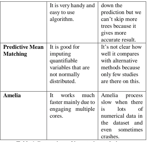
When we are dealing with different imputation techniques to handle missing data each of them will have its own positives and negatives which results in shifting to the best technique based on our requirement. Based on our understanding from all the above methods the following table is constructed with their strong and weak points.

Methods Positives Negatives

Mean Simple to

understand and to apply. Do not reduce sample size.

Sample size is overrated. Variance is underrated. Correlation is negatively biased. etc.

Median It is used over mean to assure

robustness. When the distribution of the values of a given feature is slanted it is considered over mean.

Same as Mean.

KNN KNN can predict

both qualitative attributes and quantitative attributes. It is best for instances with multiple missing values.

The choice of the distance function become difficult. Its takes much time because whole dataset will be scanned for most similar cases.

Linear regression

It is very easy and intuitive to use and understand. We can use this to find the nature of the bond between the two variables.

It assumes there is a straight

relationship between variables which is incorrect sometimes and is very subtle to the anomalies in the data.

Mice As it will produce

different number of datasets and pooled together to find the best replaceable value it is more efficient.

This is very slow process when compared to the remaining techniques.

Random Forest This can be used for both regression and classification.

It is slow process because more tress will slow

It is very handy and easy to use

algorithm.

down the prediction but we can’t skip more trees because it gives more accurate result.

Predictive Mean Matching

It is good for imputing quantifiable variables that are not normally distributed.

It’s not clear how well it compares with alternative methods because only few studies are there on this.

Amelia It works much

faster mainly due to engaging multiple cores.

Amelia process slow when there

is lots of

numerical data in the dataset and even sometimes crashes.

Table 1 Comparison of imputation techniques.

From Table 1, the pros and cons of all the 8 imputation techniques that were used in our analysis. After implementing different imputation techniques to replace the missing values with the best matching value by different techniques, each of their accuracy was examined with the help of RMSE.

A. RMSE

The RMSE is the estimated value of the standard deviation of your data. If the data is Gaussian type, and there is more than enough data, it’s a good calculation of the standard deviation. It will be bad, if the data is non-Gaussian type.

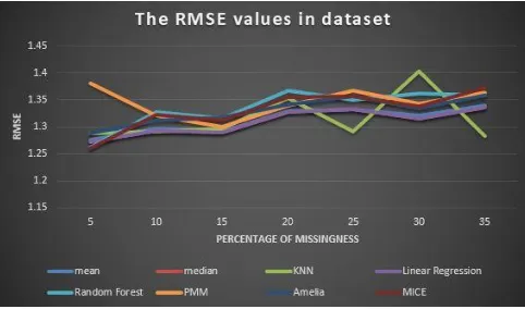
Table 2 RMSE values of imputation techniques for different percentage of missing values.

International Journal of Innovative Technology and Exploring Engineering (IJITEE) ISSN: 2278-3075, Volume-8 Issue-7, May, 2019

Figure 3The RMSE in dataset with missing ratio till 40%.

As drawn in Figure 3, accuracy of different algorithms ranges with the different amount of missingness.

V. CONCLUSION

After analyzing and implementing all the imputation techniques which discussed in this paper, accuracy of each is determined and tabulated. Based on the paper [13], the RMSE accuracy will be purely depends on the type of dataset which is considered and type of values it comprises. For the dataset which we have considered among all the algorithms implemented to impute missing data, MICE and PMM is having the constant Values of accuracy and KNN is having the values which varied the most. As whenever there comes dissatisfaction, there comes requirement for new methods. Finally all the imputation techniques will have their preference for works which it suits the best, but MICE and PMM rules the other techniques with much efficiency and accurate imputation.

REFERENCES

1. Catia M.Salgado, Carlos Azevedo, Hugo Proenca, Susana M. Vieira,

“Missing Data “Springer Journal 10 September 2016.

2. Edgar Acuna, Caroline Rodriguez, “The Treatment of Missing Values

and its Effect on Classifier Accuracy “Springer Conference Paper.

3. D.B.Rubin, “Multiple Imputation for Data-Base Construction “Springer

Conference Paper.

4. John W. Graham PhD Patricio E. Cumsille PhD Allison E. Shevock,

“Methods for Handling Missing Data” 26 September 2012.

5. Rogier T.Donders, Geert J.M.G var der Heijden, Theo Stijnen, Karel G.M

Moons, “A Gentle Introduction to Imputation of Missing Values“ Science Direct 11 July 2006.

6. Zhongheng zhang, “Missing data imputation: focusing on single

imputation “NCBI Resource January 2016.

7. Andreas Barth, Jorgen Wallerman, Goran stahl, “Spatially consistent nearest neighbor imputation of forest stand data “Science Direct 16 March 2009.

8. Quihua Wang, J.N.K Rao, “Empirical likelihood for linear regression models under imputation for missing responses “Journal of statistical software 18 December 2008.

9. Patrick Royston, Ian R. White, “Multiple Imputation by Chained

Equations (MICE): Implementation in Stata “ Journal of statistical software December 2011.

10.Anoop D. Shah, Jonathan W. Bartlett, James Carpenter, Owen Nicholas,

Harry Hemingway, “Comparison of Random Forest and Parametric Imputation Models for Imputing Missing Data Using MICE: A CALIBER Study“ Oxford Academic 12 January 2004.

11.Lawrence R, Landerman, Kenneth C. Land, Carl F. Pieper, “An

Empirical Evaluation of the Predictive Mean Matching Method for Imputing Missing Values“ Sociological Methods & Research 01 August 1997.

12.Zhongheng zhang, “Multiple imputation for time series data with Amelia

package “NCBI Resource February 2016.

13.Shichao Zhang, Zhi JIn, Xiaofeng Zhu, “Missing data imputation by utilizing information within incomplete instances “ Science Direct March 2011.

AUTHORS PROFILE

S. Deepa Kanmani currently working as an assistant professor in the stream of Computer Science and Engineering at Karunya Institute of Technology and Sciences and pursuing PhD.

Durgaprasad Nannuri is an undergraduate student in the stream of Computer Science and Engineering at Karunya Institute of Technology and Sciences.

Gopal Krishna Mupparaju is an undergraduate student in the stream of Computer Science and Engineering at Karunya Institute of Technology and Sciences.

Sravan Reddy Golamari is an undergraduate student in the stream of Computer Science and Engineering at Karunya Institute of Technology and Sciences.

Revanth Reddy Devana is an undergraduate student in the stream

of Computer Science and