https://doi.org/10.5194/angeo-36-731-2018 © Author(s) 2018. This work is distributed under the Creative Commons Attribution 4.0 License.
“Diffusion” region of magnetic reconnection: electron orbits
and the phase space mixing
Alexey P. Kropotkin
Skobeltsyn Institute of Nuclear Physics, Moscow State University, Moscow, Russia Correspondence:Alexey P. Kropotkin ([email protected])
Received: 7 November 2017 – Revised: 27 February 2018 – Accepted: 17 April 2018 – Published: 16 May 2018
Abstract.The nonlinear dynamics of electrons in the vicinity of magnetic field neutral lines during magnetic reconnection, deep inside the “diffusion” region where the electron motion is nonadiabatic, has been numerically analyzed. Test parti-cle orbits are examined in that vicinity, for a prescribed pla-nar two-dimensional magnetic field configuration and with a prescribed uniform electric field in the neutral line direction. On electron orbits, a strong particle acceleration occurs due to the reconnection electric field. Local instability of orbits in the neighborhood of the neutral line is pointed out. It com-bines with finiteness of orbits due to particle trapping by the magnetic field, and this should lead to the effect of mixing in the phase space, and the appearance of dynamical chaos. The latter may presumably be viewed as a mechanism producing finite “conductivity” in collisionless plasma near the neutral line. That conductivity is necessary to provide violation of the magnetic field frozen-in condition, i.e., for magnetic re-connection to occur in that region.
Keywords. Magnetospheric physics (plasma sheet)
1 Introduction
The problem of magnetic reconnection in the vicinity of the neutral line for collisionless plasma has an extremely exten-sive literature; see, for example, the special issue of Space Science Reviews 2011 and the work (Hesse et al., 2011) and references therein. According to the prevailing ideas, the reconnection process proper occurs in the central part of a current sheet (CS) separating the regions with oppositely directed magnetic field, and is provided by processes on a very small electronic scale in the direction zperpendicular to the CS, where the role of finite conductivity in the gen-eralized Ohm’s law assumes the effect of the nongyrotropic
component of the electron momentum flux (“pressure”) asso-ciated with the unmagnetized electron orbits on those small scales (Kuznetsova et al., 2001). The fields and fluxes of ions and electrons in the greater part of the “diffusion” re-gion, at scalesz of the order of the ion inertial length di, z∼di=c/ωpi (c is the speed of light, ωpi=
p
4π nie2/mi is the ion plasma frequency), but outside a very small re-gion, where even the electrons cease to be magnetized and the nongyrotropic component of the electron momentum flux (“pressure”) appears, may be described in the Hall MHD terms. The scale of the “diffusion” regionin the direction of plasma outflow(along thex direction parallel to the CS and lying in the magnetic field plane) and, correspondingly, the reconnection rate, are determined by the inflowing con-vection velocity times the reconnecting (Bx) component of
the magnetic field. And those are “tied” into equations de-scribing the system macroscopically. Such adjustment of the processes in the vicinity of the neutral line to external condi-tions occurs at two different levels, ionic and electronic. On a larger scale, in most of the “diffusion” region, forz∼di, the fields and fluxes of ions and electrons, as has been men-tioned, are determined by the Hall MHD equations. At the smallest scale, in a region where the electrons are not mag-netized and the electron pressure is nongyrotropic, the elec-tron flux profile along thex direction is adjusted in such a way that the nongyrotropic electron pressure component is just sufficient to maintain the electric field that sets the re-connection rate on the neutral line, but is determined by the macroscopic flow.
dissipation (Hesse et al., 2001; Liu et al., 2017). A fairly sim-ple qualitative explanation can be given to that. It turns out that the outflow of the electron fluid from the inner (dissipa-tion) region has the character of a strong standing whistler wave. The phase velocity of the whistlerω/ kwith which the outflow occurs is inversely proportional to the spatial scale, ω/ k∼k∼1/L. This means that the electron flux from the dissipation region, which determines the magnetic reconnec-tion rate, being the product of the velocity and thickness of the layer∼L, isindependent of this thickness. But it is just this scale that is regulated by the intensity of the dissipative effect: the resistivityηin the collisional case or the value of the nongyrotropic electron pressure in the collisionless one. Thus the layer structure adjusts to the magnetic reconnection rate, but does not affect it.
Note, however, that such a situation does not mean that the real nature of electron dynamics and corresponding fea-tures of electron orbits, which lie at its basis, may be thought insignificant.
Outside the diffusion region, the process of “magnetic an-nihilation” – the transformation of electromagnetic energy into the energy of plasma flows, meaning magnetic reconnec-tion in the wider sense, is determined by ion moreconnec-tions, includ-ing those that are substantially nonadiabatic in thin layers ad-jacent to the diffusion region. As was pointed out in Domrin and Kropotkin (2007a, b, c), Kropotkin and Domrin (2009), and Kropotkin (2013), in that region the process is domi-nated by an “anisotropic” CS, the structure of which is deter-mined by the specific ion orbits. This leads to ion anisotropy of a certain type, dependent on the distance from the cen-tral plane. However, inside the diffusion region the process of magnetic reconnection requires an “intermediary”, an ad-ditional link. This is the abovementioned Hall MHD struc-ture, based on specific differences between the electron and ion orbits. And finally, deep inside this layer, in the nearest neighborhood of the neutral line, unmagnetized electron or-bits determine the dynamics and structure of the reconnecting CS.
It is precisely the specific nature of such orbits, which in previous studies has remained mostly unidentified in a proper perspective, that this paper is devoted to. Basically, the numerical approach applied in this paper differs only weakly from that adopted in a number of earlier studies (Martin, 1986; Burkhart et al., 1991, and references therein). Moreover, the chaotic particle dynamics were then identi-fied numerically by means of Lyapunov characteristic expo-nent analysis. However, the insight which appeared since that time, concerning the role of the electron zone in the “diffu-sion region”, on the one hand, and penetration of the nonlin-ear dynamics and dynamical chaos notions into this resnonlin-earch area, on the other hand, has laid the way to a number of new results.
In this paper, the nonlinear dynamics of electrons mov-ing in a magnetic field near its neutral line and in an electric field corresponding to the inflow of plasma into the
recon-nection zone has been studied numerically in a wide range of determining parameters (Sect. 2). Of course, these dynam-ics do not obey the adiabatic theory; its important property is a strong particle acceleration near the field neutral line. An-other important feature of particle dynamics near the neutral line is pointed out in Sect. 3. Analysis of an equation govern-ing such dynamics, involvgovern-ing the numerical results of Sect. 2, indicates an exponential divergence of orbits starting closely nearby. This feature of local instability, along with finiteness of the orbits in the phase space, in the general theory of non-linear dynamical systems, should result in the appearance of stochastization, i.e., of dynamical chaos in the system. This is discussed in Sect. 4 in terms of the phenomenon of mixing in the phase space and formation of the collisionless energy dissipation mechanism. In this way we obtain a corroboration on the side of microscopic dynamics that the diffusion region should have a dissipation property in the macroscopic sense, i.e., provide the transformation of electromagnetic energy (a nonzero Poynting vector in the inflow region) into energy of accelerated particles.
2 Electron orbits: numerical simulation
We study test particle orbits in a prescribed field configu-ration. We use a two-dimensional model of magnetic field B(x, z)with a neutral line,B(0,0)=0:
Bx=qbz;By=0;Bz=
b
κarctg (κx) .
Here the parameter q≥1 determines the opening an-gle, i.e., the angle between the separatrices dividing the magnetic fluxes near the neutral line, and also the value of a finite current density in the y direction, jy=
cbhq− 1+κ2x2−1/2i/4π. The normal component Bz
goes to a constant for large values ofx. In the calculations, dimensionless variables (ξ, η, ζ, τ) are used:
x= mc T ebξ;y=
mc T ebη;z=
mc
T ebς;t=T τ,
eand mbeing the electron charge and mass, respectively. HereT is an arbitrary timescale, which we choose based on the requirement of the best visibility in the presentation of results; see below. We also introduce the dimensionless pa-rameterk=T eb
mcκ. In what follows, for convenience, we
re-name the variables (ξ, η, ζ, τ) back to(x, y, z, t ), andkback toκ; then in dimensionless variables we have the equations of motion:
¨
x−arctg (κx) κ y˙=0; ¨
y+arctg (κx)
κ x˙−qzz˙−ε=0; ¨
z+qzy˙=0.
(1)
Here
ε=T3e 2b
is a dimensionless analog of the value meE0, where E0= const is the intensity of the electric field directed along y. (At small z and x (0)→0 the motion along y oc-curs mainly under action of an accelerating force eE0 so that dy/dt∼eE0t /m. We obtain as a result that the equa-tion d2z
dt2 + eb mcqz
dy
dt =0 describes oscillations over z with
their frequency square given approximately by the formula ω2=e2bqE0t /m2c. Therefore, requiring that in the time interval T of the equation set integration, there should be many oscillations, and we obtain the conditionε=ω2T2= e2bqE0T3/m2c1. As to the magnitudeezof oscillations,
we haveez∼vz/ω. The value of velocity vz at the
begin-ning of the oscillation regime is given by an estimate vz∼
cE0/Bx∼cE0/2bz. It follows thatez
2∼cE0 2bω=
m2c2 2qe2b2T2
√ ε, and for the dimensionless magnitude we have an estimate
e
ς2=(ebT /mc)2ez2=√ε/2q. It is seen that taking the ε value to be quite large we can obtain a demonstrable rep-resentation of the system dynamics at smallx (0), at those times when the particle arrives in close vicinity of the mag-netic field neutral line.)
Equations (1) must be supplemented by initial conditions, i.e., by setting the valuesx(0),y(0),z(0),x(0),˙ y(0),˙ z(0).˙ In the planar geometry, without loss of generality we assume y(0)=0.
We have studied a set of possible orbits over a wide range of parameters, including the valuesκ,q,εand initial values of coordinates and velocities. To illustrate the typical results here, we have chosen the values of the magnetic field param-etersκ=0.002, q=2.
In the simplest situation, it can be assumed that a flow of plasma with cold electrons arrives at the CS. Then, if an electron starts somewhere away from the CS, it must be postulated that its velocity v0(0) in the local reference frame (that moving with the plasma bulk velocity) is zero. Thus we have two conditions: E0+[v(0)×B(0)]/c=0, and(v(0)B(0))=0. In the dimensionless variables this leads to the following relations:
˙
x (0)=arctg (κx (0)) κ
ε
q2z2(0)+arctg2(κx (0)) /κ2; ˙
y (0)=0; ˙
z (0)= −qz (0) ε
q2z2(0)+arctg2(κx (0)) /κ2.
(3)
For this simplest situation, it can be easily seen how the di-mensionless parameters that determine the orbit of interest should be chosen. Since we will further investigate the de-pendence of the orbit features on the initial valuex(0) start-ing withx(0)=0, there is actually only a pair of such dimen-sionless parameters, z(0)and ε. For an arbitrary timescale T, it is to be assumed that the time a particle takes to reach the plane z(0)=0 must be much less than this scale: z(0)/cE0
bz(0)T (here z(0) has the original meaning, with
the dimension of length). Then, taking into account Eq. (2) and using our reverse renaming of variables, the condition εz2(0)is obtained. Accordingly, we shall first consider
the electron orbits at ε=50 000 and specifying the initial value of the coordinatez(0)=50.
For solution of the Equation set (1) with corresponding initial conditions and for graphical presentation of results, the Wolfram Mathematica package has been used. Accuracy of the codes applied in Mathematica calculations was of course adequately verified by the Wolfram team long ago; it is quite sufficient for the presented graphics. In our work, in some cases that accuracy has been tested by means of varying the parameters used.
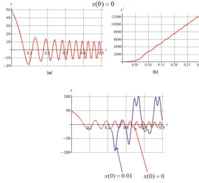
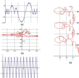
First of all, let us turn to the casex(0)=0. According to Eq. (3) we havex(0)˙ =0, and it is clear that the orbit remains in the planex=0, while in theydirection anunlimited ac-celerationtakes place. The corresponding time profilez(t )is shown in Fig. 1a. Apparently, this is a “Speiser” orbit oscil-lating near the neutral layer, complicated by acceleration in the electric fieldEy=E0=const. This acceleration occurs
at an almost constant rate from the momenttcwhen the par-ticle reaches the neighborhood of the neutral line, as can be seen from Fig. 1b. Acceleration isunlimited in time.
Now consider the results of numerical calculations relat-ing to how the electron orbits in general look and how their character changes when the initial conditions change. From a large number of calculations performed, here we illustrate several characteristic series.
Consider in more detail the orbits discussed above: we set againε=50 000 and z(0)=50, and let the initial displace-mentxfrom the planex=0 be very small,x(0)=0.01.
An initial course of thez(t )function is shown in Fig. 1c, for the starting casex(0)=0 (red curve) and forx(0)=0.01 (blue curve). The initial motion to thez=0 plane and the first meandering “Speiser” oscillations in these two cases are indistinguishable. But then we see a sharp departure of a par-ticle from the “Speiser” orbit; the oscillation pattern com-pletely changes. This may be generally viewed as manifes-tation of local instability in the phase space, as we discuss below, in Sect. 3.
Figure 1. (a) Oscillations overzatx(0)=0.(b)Time dependence of the velocityy (t )˙ atx(0)=0.(c)Comparison of the initial time dependencez(t )forx(0)=0 (red curve) andx(0)=0.01 (blue curve).
Having presented in Fig. 2d a plot of time dependence for the particle kinetic energy m˙
x2(t )+ ˙y2(t )+ ˙z2(t )/2 (in arbitrary units), we see that at first, when the particle moves to the z=0 plane, this energy remains small, and then the particle is very quickly accelerated by the electric field E0 on the “Speiser” section of the orbit, and after this the energy remains almost constant, only slightly increasing with each new intersection of thez=0 plane. The fast acceleration oc-curring on the “Speiser” portion of the orbit is nowlimited in time, in contrast to the casex(0)=0.
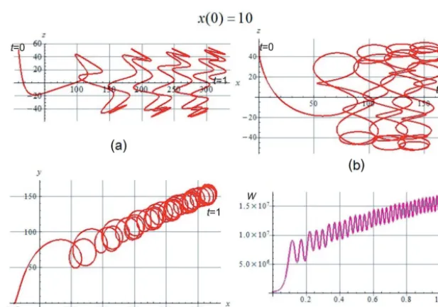
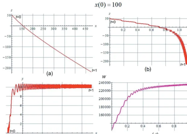
The orbits of electrons that are “cold” at the start re-tain a similar character up to the valuesx(0)∼1. However, for larger x(0) values, the situation changes significantly. We present for comparison the corresponding plots for the x(0)=10 case. The orbit in projection onto the(x, z)plane is shown in Fig. 3a, in projection onto the (y, z) plane in Fig. 3b, and in projection onto the (x, y) plane in Fig. 3c. Figure 3d demonstrates the time dependence of the kinetic energy. It is seen that there is no “Speiser” section here, but the orbit remains finite overz, oscillating between the reflec-tion points, with a gradual energy gain. At the first intersec-tion of thez=0 plane, a particularly fast acceleration occurs. With an even greater initial distance from thex=0 plane, x(0)=100, the orbit has again a pattern different from the previous ones. The corresponding plots are shown in Fig. 4a– c. Here the orbit crosses thez=0 plane only once, and then leaves it winding around a field line; this is accompanied by slow drift motions in the direction transverse to that of
mag-netic field in the central plane. Acceleration occurs only at this one-time intersection, and the kinetic energy achieved is much less than in the previous calculations, where accelera-tion occurs during multiple intersecaccelera-tions of thez=0 plane; see the plot in Fig. 4d.
When specifying nonzero initial speedsv06=0 in the local frame moving with the plasma bulk velocity, orbits appear that do not intersect thez=0 plane at all, and there is no ac-celeration. This behavior corresponds to the familiar pattern of electric drift in the vicinity of the neutral line, and arises with a small oscillatory component of the particle velocity characteristic of “cold” electrons: the electric drift forms par-ticle orbits along hyperbolas orthogonal to the magnetic field line hyperbolas.
So, in general, for all variations of the parameters, we ob-serve the same effect: acceleration of electrons by the electric field when they appear in the vicinity of the neutral line; the picture is somewhat different for a single or multiple inter-section of the neutral plane. At very smallx (0), there is a distinctly “Speiser” section of the orbit, on which a particu-larly fast acceleration takes place.
3 Local instability
[image:4.612.156.442.67.330.2]nu-Figure 2.The orbit pattern atx(0)=0.01:(a)projected to the(x, z)plane,(b)projected to the(y, z)plane,(c)projected to the(x, y)plane.
[image:5.612.144.451.67.277.2](d)Time dependence of the kinetic energy.
Figure 3.The orbit pattern atx(0)=10:(a)projected to the(x, z)plane,(b)projected to the(y, z)plane,(c)projected to the(x, y)plane.
(d)Time dependence of the kinetic energy.
merical result that, beginning at somet=tc, the velocityvy
increase is very close to linear; see Fig. 1b. For values of x (0)6=0 that are small compared toκ−1(the diffusion re-gion scale in the x direction),κx (0)1, and returning to the initial variables, we then have
¨ x= e
mcvyBz= e2b
m2cE0x (t−tc)=
x (t−tc) τ3 ,
where
τ=
e2b m2cE0
−1/3
=
eb
mc
−2/3c
bE0
−1/3
.
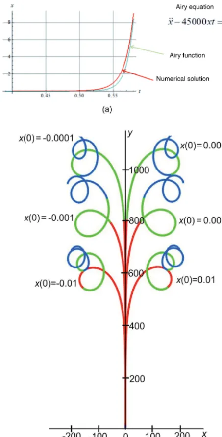
Note that the above equation is the Airy equation. In our di-mensionless variables it takes the form
¨
x−45 000xt=0.
[image:5.612.141.450.330.546.2]Figure 4.The orbit pattern atx(0)=100:(a)projected to the(x, z)plane,(b)projected to the(y, z)plane,(c)projected to the(x, y)plane.
(d)Time dependence of the kinetic energy.
x=0 plane is described by the Airy function of the second kind x(t0)=x(0)Bi 10×451/3t0
(where t0=t−tc) with an exponential asymptotic. This is shown in Fig. 5a, which presents the results of calculating the above Airy function (blue curve) and of the numerical solution of the Equation set (1) for x(t ) (red curve). (In the Figure x(0)=0.01 is adopted.)
Now for any small deviationξ (t )=x1(t )−x (t ), for a pair of orbits starting at small initialx (0)6=0 andx1(0)6=0, we obtain the same governing equation, and the following argu-ment may be applied to such a deviation.
On a small time interval 1t the coefficient at x in the equation, equal to κ= e2b
m2cE0t=(t /τ ) τ
−2 changes by e2b
m2cE0
1t=(1t /τ ) τ−2, and its relative variation is 1κ/κ∼1t /t. If the coefficient κ remained con-stant, there would exist an exponentially increasing so-lution ∼exp κ1/2t
. The exponent is equal to κ1/2t=
e2b m2cE0
1/2
t3/2=(t /τ )3/2, and on the time interval 1t it changes by 32τ−3/2t1/21t.
So if we fix some time moment tτ, then on the time interval from t to t+1t the exponent changes by
3 2τ
−3/2t1/21t=3 2(t /τ )
1/2(1t /τ )1t /τ. Therefore if the double inequalityt1tτ holds, we obtain a very large value of the exponential multiplier exp32τ−3/2t1/21t1 along with a small variation of κ (that coefficient remains almost constant, 1κ/κ∼1t /t1), i.e., at every tτ a fast, exponential divergence of orbitsx (t )andx1(t )occurs. In other words, if we take a pair of closely neighboring orbits at a momentt, then during particle motion along them at later
times, earlier than the dynamical equation form changes con-siderably, the particles will diverge at an exponentially large distance.
In such a situation we may speak of the presence of alocal instabilityin the system, in the vicinity of the magnetic field neutral line.
A clear confirmation of instability atx(0)= ˙x (0)=0 is shown in Fig. 5b, where the orbits starting at different small |x(0)|values are shown projected onto thez=0 plane. Here the orbit sections fromt=0 tot=0.2 are shown in red, from t=0.2 tot=0.4 – in green, and fromt=0.4 tot=0.45 – in blue.
Note that the diverging orbits turn out to be limited (gen-erally speaking, in the phase space) because of cyclotron ro-tation.
4 Discussion and conclusions
As has been shown earlier (see, e.g., Burkhart, 1990), the motion of an electron in the neutral line vicinity being nona-diabatic, is described by nonlinear equations, and on the orbit there is a “Speiser” meander section on which a fast particle acceleration occurs, in the electric field corresponding to the inflow of plasma into the reconnection area. This should re-sult in a strong conversion of energy of the electromagnetic field into energy of the electron flows.
Figure 5. (a)Time dependencex (t )at smallx (0)6=0.(b)Orbits starting at various small values ofx(0), projected to the planez=0.
It is well known that even in the case of a relatively simple system of low dimension, there may exist such domains in its phase space, where the orbits are stochastic. We point out that an electron in our model field, in the neutral line vicinity is just such a system.
Consider a pair of orbits in theXphase space (with dimen-sionn)starting at closely located pointsX(0)andX1(0)so that ξ(0)=X1(0)−X(0)→0. We then can linearize the equation set of the dynamical system and obtain a set of lin-ear equations for the small incrementξ(t ). LetAbe the ma-trix of coefficients of that equation set. The general solution of the equation set may be presented as a superposition ofn
fundamental particular solutionsξj(t ) :
ξ(t )=X
j
Cjξj(t ) ,
where theCj constants are determined from the projection
of the initial increment ξ(0) onto the
ξj(0) vector ba-sis. In the simplest case when the matrix of coefficientsA is independent of time, all the vector componentsξj(t )are exponential in time, ξj(t )∼exp λjt. The parameters λj
areLyapunov’s exponentsof the system. Generally, the time dependence of the fundamental particular solutionsξj(t )
is more complicated than exponential. However, keeping in mind that the A(t )matrix does not unlimitedly grow with time, for large times we can writeξj(t )
=8j(t )exp λjt
, where the8j(t )function has a slower growth rate than
ex-ponential.
Turning back to our case, we have seen in Sect. 3 that in the neutral line vicinity there is an area in the phase space where local instability acts. It means that the dis-tance ξ between neighboring orbits in the x direction in-creases exponentially: on a time interval1t it increases so that ξ (t+1t ) /ξ (t )=exp32τ−3/2t1/21t1. We con-clude that a maximumpositiveLyapunov’s exponent should exist,λ(m)≥3
2τ
−3/2t1/2.
Note that the existence of local instability, in the terms of a positive Lyapunov characteristic exponent, was first pointed out for this problem in Martin (1986).
As has been noted earlier, the local instability of orbits takes place along with finiteness of motion in the phase space due to the particle trapping by the magnetic field. From the general theory of nonlinear dynamical systems (see, e.g., Ta-bor, 1989; Ott, 2002; Usikov et al., 1988) it then follows that the system possesses the corresponding Kolmogorov–Synai entropy of the order of the maximum positive Lyapunov ex-ponent,h∼λ(m). This means that correlation decay occurs on the timescale
τ(corr)≤
2 3τ
3/2t−1/2∼mc eb
b
cE0
1/2
t−1/2.
This leads to the effect of mixing in the phase space, and to the appearance of dynamical chaos on some particular sites in the phase space.
[image:7.612.53.280.66.512.2]Figure 6. (a)Oscillations overzon the “cucumber” orbit.(b)The “cucumber” orbit projected to thez=0 plane.(c)Oscillations overzon the “ring” orbit.(d)The “ring” orbit projected to thez=0 plane.
radius in the field B0) is small, then there is a stochastiza-tion mechanism associated with the intersecstochastiza-tion of the sepa-ratrix between two different types of fast oscillations, spiral and meander (Büchner and Zelenyi, 1986; Timofeev, 1978; Neishtadt, 1987). And with the increase of the parameterκ, according to Malova and Sitnov (1989), stochastization addi-tionally occurs due to overlapping resonances of the fast and slow oscillations.
If in the model we are considering, with a nonuniformBn field, with a neutral line of the magnetic field, we set the elec-tric fieldE0equal to zero, then the nature of orbits described in these previous works is basically preserved (see Fig. 6a– d), supplemented only by the particle displacement over y due to the drift in the Bn field, nonuniform overx. There-fore, the same mechanisms of stochasticity must operate.
However, in the model considered here, in the presence of a reconnection electric field, those effects, as we have seen, are supplemented by the local instability effect near the neu-tral line. A qualitative explanation may be given following the notions of, for example, Usikov et al. (1988) concern-ing the role in the effect of stochasticity generation which is played by a separatrix existing in the phase space of a non-linear system. “Slow” oscillations over x occur within cer-tain limits from xmin up toxmax. Ifxmincorresponds to the
position of the neutral line of the magnetic field, a separatrix arises on which the period of “slow” oscillations tends to in-finity. Accordingly, a “phase space fluid drop” of this “slow” variable is stretched in phase (and compressed in action), and phase mixing occurs (e.g., Usikov et al., 1988). Combined with the finiteness of the orbits, this provides a mechanism of stochastization.
According to modern knowledge (see, for example, Gas-pard, 1998)macroscopictransport processes in multiparticle systems may be viewed as being based onmicroscopic parti-cle dynamics, which demonstrates the properties of dynam-ical chaos. Accordingly, the above argument seems to indi-cate the presence of collisionless “dissipation” of the Landau damping type (Mouhot and Villani, 2011). As this mathe-matical research shows, the phenomenon of damping can be interpreted in terms of the transfer of regularity from kinetic variables to spatial ones, and not as a transformation of en-ergy;phase mixingis the clue mechanism.
[image:8.612.144.450.70.372.2]Now we note an analysis somewhat similar to ours was recently carried out in Zenitani and Nagai (2016). A set of electron orbits passing in the vicinity of the magnetic field neutral line has been identified there under conditions when this field itself, as well as the electric field and the plasma characteristics, is determined in numerical simulation of the entire three-dimensional plasma system. Modeling was car-ried out by means of a particle-in-cell code applied to a time-dependent spontaneous magnetic reconnection process in which an electric field arises in a self-consistent manner as a result of development of an initially small perturbation, rather than being arbitrarily given, as is done here.
Electron orbits are grouped in this work according to some of their basic characteristics. There are classes of or-bits qualitatively corresponding to those obtained by us, with “Speiser” sections and fast acceleration in the vicinity of the neutral line. Along with them, orbits of a substantially dif-ferent type, named “Speiser orbits without intersection of the central plane”, were obtained. Those orbits appear due to the fact that in the model (Zenitani and Nagai, 2016) there are such electric fields that are absent here: the polarization field Ez and the parallel field Ek. Such fields actually arise
dur-ing magnetic reconnection, due to the Hall plasma dynamics indicated in Sect. 1.
However, the approach used in Zenitani and Nagai (2016) does not allow the systematic tracing of how the orbit nature and the acceleration gained by an electron depend on the dis-tance to the neutral line, as we have done here. This depen-dence could not be traced down to very small x (0)values where the local instability appears. So the local instability of orbits in the vicinity of the neutral line was not identi-fied; this has been done here for the first time. As indicated above, combined with the finiteness of motion in the phase space due to the particle trapping by the magnetic field, this instability serves as the basis for the effect of the phase space mixing and the appearance of dynamical chaos.
One more important point, which has a wider relation to particle-in-cell (PIC) codes, is that the formation of a small-scale (fractal) stochastic structure in the phase space cannot be reproduced in numerical simulation by means of alarge particle-in-cell code. But namely such a structure is appar-ently responsible for the dissipative behavior of the system in the vicinity of the magnetic field neutral line, in a thin elec-tronic “diffusion layer”. True, this flaw of PIC codes may be partly overcome if the particle number per cell becomes sufficiently large, since as this number increases the size of super-particles in the PIC method decreases.
An additional comment should be made here, in particular in relation to self-consistent models of magnetic reconnec-tion. In fact it is just assumed that any electron orbit under study is located deep inside the small electron diffusion re-gion. There is no attempt to relate the adopted dimensionless parameters to physical scales characteristic for that domain. True, this is an ambiguous task since those scales depend in particular on the (numerical) model adopted for such a
com-parison. In any case it is reasonable to postulate that such a small electron diffusion region exists. Note, however, that if the current carried by unmagnetized electrons themselves were large, then the magnetic field configuration would be more complicated: it would have a spatial scale of the same order as the electron oscillations about the neutral plane of the CS. Then a study based on test particle orbits in a pre-scribed field would be inapplicable. So another assumption, implicitly made, is that the currents forming the magnetic field configuration, are carried mainly by ions, and not by unmagnetized electrons; correspondingly, the field configu-ration spatial scales are sufficiently large. This actually is the case for the existing self-consistent models of magnetic reconnection (e.g., Hesse et al., 2011; Bessho et al., 2014; Liu et al., 2017). This may also eliminate the problem with those electric fields mentioned above which appear in self-consistent models, the polarization fieldEzand the parallel
fieldEk. Those fields vary on a large ionic scale; in
particu-lar, the polarization field is associated with the Hall electric current (Hoshino, 2005). Also, in the numerical simulation (Egedal et al., 2012) it was found out that the parallel fields operate in spatial regions that exceed the regular electron dif-fusion region scale by orders of magnitude. And then, since unlike the reconnection fieldE0, those fields must go to zero atz→0, they might be neglected in the small electron diffu-sion region.
Magnetic reconnection in collisionless plasma may be considered as a complex of two main problems. The first problem is fast energy conversion. As has been shown in earlier studies and has been pointed out in the Introduction, this may be understood as a result of “magnetic field anni-hilation” dominated by an “anisotropic” thin current sheet, the structure of which is determined by thespecific ion or-bits. The second problem is that of a nonzero electric field E6=0 on the magnetic field neutral lineB=0. This is shown here to be directly connected with specific features of elec-tron motion. Electrons are accelerated by the electric field, dvy
/dt >0 in the “electron diffusion region” where they
are “demagnetized”. The resultingvy
produces a repulsing
Lorentz force acting in thexdirection, and alocal instability appears. Combined with finite dimensions of the electron or-bit in the phase space (due to magnetic trapping) this leads to orbit stochastization. The latter may presumably be viewed as a mechanism producing finite “conductivity” in collision-less plasma near the neutral line.
Data availability. No data sets were used in this article.
Competing interests. The author declares that they have no conflict of interest.
References
Bessho, N., Chen, L.-J., Shuster, J. R., and Wang, S.: Electron dis-tribution functions in the electron diffusion region of magnetic reconnection: Physics behind the fine structures, Geophys. Res. Lett., 41, 8688–8695, https://doi.org/10.1002/2014GL062034, 2014.
Büchner, J. and Zeleny, L. M.: Deterministic chaos in the dynamics of charged particles near a magnetic field reversal, Phys. Lett. A, 118, 395–399, 1986.
Burkhart, G. R., Martin Jr., R. F., Dusenbery, P. B., and Speiser, T. W.: Neutral line chaos and phase space structure, Geophys. Res. Lett., 18, 1591–1594, 1991.
Chen, J. and Palmadesso, P. J.: Chaos and nonlinear dynamicsof
single-particle orbits in a magnetotaillike magnetic field, J. Geo-phys. Res., 91, 1499–1508, 1986.
Domrin, V. I. and Kropotkin, A. P.: Dynamics of equilibrium up-set and electromagnetic energy transformation in the geomag-netotail: a theory and simulation using particles, 1. Evolution of configurations in an MHD approximation, Geomagn. Aeron., 47, 299–306, 2007a (English translation).
Domrin, V. I. and Kropotkin, A. P.: Dynamics of equilibrium upset and electromagnetic energy transformation in the geomagneto-tail: a theory and simulation using particles, 2. Numerical sim-ulation using particles, Geomagn. Aeron., 47, 307–315, 2007b (English translation).
Domrin, V. I. and Kropotkin, A. P.: Dynamics of equilibrium upset and electromagnetic energy transformation in the geomagneto-tail: a theory and simulation using particles, 3. Versions of for-mation of thin current sheets, Geomagn. Aeron., 47, 555–565, 2007c (English translation).
Egedal, J., Daughton, W., and Le, A.: Large-scale electron accelera-tion by parallel electric fields during magnetic reconnecaccelera-tion, Nat. Phys., 8, 321–324, 2012.
Gaspard, P.: Chaos, scattering and statistical mechanics, Cam-bridge, University Press, 1998.
Hesse, M., Kuznetsova, M., and Birn, J.: Particle-in-cell simulations of three-dimensional collisionless mag-netic reconnection, J. Geophys. Res., 106, 29831, https://doi.org/10.1029/2001JA000075, 2001.
Hesse, M., Neukirch, T., Schindler, K., Kuznetsova, M., and Zeni-tani, S.: The diffusion region in collisionless magnetic reconnec-tion, Space Sci. Rev., 160, 3–23, https://doi.org/10.1007/s11214-010-9740-1, 2011.
Hoshino, M.: Electron surfing acceleration in mag-netic reconnection, J. Geophys. Res., 110, A10215, https://doi.org/10.1029/2005JA011229, 2005.
Kropotkin, A. P.: Processes in current sheets responsible for fast energy conversion in the magnetospheric collisionless plasma, 80 pp., http://arxiv.org/abs/1302.2795, 2013.
Kropotkin, A. P. and Domrin, V. I.: Kinetic thin current sheets: their formation in relation to magnetotail mesoscale turbulent dynam-ics, Ann. Geophys., 27, 1353–1361, 2009.
Kuznetsova, M. M., Hesse, M., and Winske, D.: Collisionless re-connection supported by nongyrotropic pressure effects in hy-brid and particle simulations, J. Geophys. Res., 106, 3799–3810, 2001.
Liu, Y.-H., Hesse, M., Guo, F., Daughton, W., Li, H., Cassak, P.-A., and Shay, M.-A.: Why does steady-state magnetic reconnection have a maximum local rate of order 0.1?, Phys. Rev. Lett., 118, 085101, https://doi.org/10.1103/PhysRevLett.118.085101, 2017. Malova, H. V. and Sitnov, M. I.: Nonlinear structures, stochastic-ity and intermittency in the dynamics of charged particles near a magnetic field reversal, Phys. Lett. A, 140, 136–139, 1989. Martin Jr., R. F.: Chaotic particle dynamics near a
two-dimensional magnetic neutral point with application to the geomagnetic tail, J. Geophys. Res., 91, 11985, https://doi.org/10.1029/JA091iA11p11985, 1986.
Mouhot, C. and Villani, C.: On Landau damping, Acta Math., 207, 29–201, https://doi.org/10.1007/s11511-011-0068-9, 2011. Neishtadt, A. I.: On the change in the adiabatic invariant on
cross-ing a separatrix in systems with two degrees of freedom, J. Appl. Math. Mech., 51, 586–592, https://doi.org/10.1016/0021-8928(87)90006-2, 1987.
Ott, E.: Chaos in Dynamical Systems, Cambridge University Press, 393 pp., 2002.
Tabor, M.: Chaos and Integrability in Nonlinear Dynamics, John Wiley and Sons, 384 pp., 1989.
Timofeev, A. V.: On the constancy of an adiabatic invariant when the nature of the motion changes, Zh. Eksp. Teor. Fiz., 75, 1303– 1308, 1978.
Usikov, D. N., Sagdeev, R. Z., and Zaslavsky, G. M.: Nonlinear Physics: From the Pendulum to Turbulence and Chaos, Contem-porary Concepts in Physics Series ISSN 0272-2488, Harwood Academic Publishers, 1988.