Characterizing spatial-spatial-spectral MRI

(1)

Theses Thesis/Dissertation Collections

1998

Characterizing spatial-spatial-spectral MRI

Kenneth Brodeur

Follow this and additional works at:http://scholarworks.rit.edu/theses

This Thesis is brought to you for free and open access by the Thesis/Dissertation Collections at RIT Scholar Works. It has been accepted for inclusion in Theses by an authorized administrator of RIT Scholar Works. For more information, please [email protected].

Recommended Citation

(2)

SIMG-503

Senior Research

Characterizing Spatial-Spatial-Spectral MRI

Final Report

Kenneth Michel Brodeur

Center for Imaging Science

Rochester Institute of Technology

May 1998

(3)

Table of Contents

Abstract 1. Copyright 2. Acknowledgments 3. Introduction 4.

Background and Significance 5.

Theory 6.

Understanding the Data Space

The Concept of Projections

Limitations and Artifacts of the Procedure

Methods 7.

Phantom Construction

Data Collection

Sinogram Construction

Width at Half-Height

Determining Point-Spread

Results 8.

Image Attributes

Presentation of Results

Peak A

(4)

Peak C

Peak D

Discussion 9.

Conclusions 10.

References 11.

List of Symbols 12.

Appendix 13.

(5)

Characterizing Spatial-Spatial-Spectral MRI

Kenneth Michel Brodeur

Abstract

Spatial-spatial-spectral magnetic resonance imaging (MRI) is a technique that produces spectral information for every volume element (voxel) in a tomographic image. Servoss and Hornak recently developed a technique for acquiring spatial-spatial-spectral images on a clinical imager. The

technique is based on projections through a spatial-spectral domain. Because resolution diminishes with shortened imaging time, it is necessary to determine the optimal imaging time for a desired resolution. The spatial-spectral resolution of this technique was determined using a chemical phantom with well-known spectral and spatial signatures. Resolution was determined as a function of the number of projections. The optimization of spatial resolution using this technique was achieved using 80 projections (using 40 MRI scans), while accomplishing similar results in the spectral domain required that 80 projections (40 MRI scans) be used. To illustrate these results, plots of the point spread function as a function of number of projections and time are presented.

(6)

Center for Imaging Science

Rochester Institute of Technology

Rochester, NY 14623-5604

This work is copyrighted and may not be reproduced in whole or part without permission of the Center for Imaging Science at the Rochester Institute of Technology.

This report is accepted in partial fulfillment of the requirements of the course SIMG-503 Senior Research.

Title: Spatial-Spatial-Spectral MRI. Author: Kenneth Michel Brodeur Project Advisor: Joseph P. Hornak SIMG 503 Instructor: Joseph P. Hornak

(7)

Characterizing Spatial-Spatial-Spectral MRI

Kenneth Michel Brodeur

Acknowledgments

This document is a testament to the support, guidance and understanding of the following wonderful people:

Mom, Dad, Erin, Pago, Mago, Winston, and George - thank's for letting me grow a little Brianne - my beautiful fiancee, no one should have to put up with a scientist

Nikki, Captain O'Brian and the triplets - you make me feel at home

The brothers of Kappa Delta Rho - thanks for the encouragement to achieve

Bro. Charles Wanda S.M. - for the gift of Wandaism, when perfectionism is just too much Greg - because getting here was just half the fun of RIT

Dr. Joseph Hornak and Thomas Servoss - the original conspirators of the project

(8)

Characterizing Spatial-Spatial-Spectral MRI

Kenneth Michel Brodeur

Introduction

This research project supports a parent project that is focused on the development of a reliable means for the production of spatial-spatial-spectral images using a magnetic resonance imaging (MRI) system. The

advantage provided by spatial-spatial-spectral imaging over traditional MR imaging is founded in its ability to reveal the chemical composition of materials that lie in a certain spatial dimension of a subject. As an example, the possibility exists that a malignant and a benign tumor - both appearing as areas of brightness in a traditional MRI - may be differentiated from each other based on their unique material properties as identified by the spectral information provided by the spatial-spatial-spectral image.

In current practice, in order to confirm a tumor to be benign or malignant, a biopsy must be taken after a traditional MRI has identified the presence of a tumor. It is speculated that the need to conduct such invasive practices may be reduced through the application of this spatial-spatial-spectral process. Ultimately, this could make the method of cancer screening less bothersome, thereby encouraging people to seek evaluation in lieu of the previous, less comfortable alternatives.

As a primary aim of this project, the time a patient spends in a MR imager will be related to a relative spectral resolution and spatial resolution. Magnetic resonance imaging machines are expensive, and most hospitals will own no more than one. Because of the non-invasive nature of the MRI process in diagnostics, the use of such a machine is in high demand. The time demand will be especially costly in the case of

spatial-spatial-spectral imaging, which requires multiple images to be acquired to construct the final image. However, different applications of this imaging process may require different levels of spatial or spectral resolution. Clinicians and doctors will be able to anticipate the time involved in imaging a subject at a certain resolution by using techniques that this project will develop for relating the number of projections used to create a spatial-spectral image and the time required to acquire that number of projections. In this way, the application of a MR spatial-spectral scan can be appropriately matched to the maximum allotted time for which the MRI may be used. This ability will be advantageous in maximizing the availability of these expensive and high demand machines.

Table of Contents

Background and Significance

(9)

plane. Materials return a signal with an amplitude corresponding to the material spectral response. In real clinical applications of the MRI process, a radio frequency (RF) pulse in conjunction with a slice selective magnetic field gradient is used to select the plane of interest. This pulse aligns the molecular magnetic spins of the materials in each plane. The rate at which these spins precess about their magnetic isocenter is constant in a uniform magnetic field. Applying the phase encoding pulse, which is a magnetic field with some gradient, allows us to identify the position of each volume element by creating a slight offset in the alignment of the molecular spin, relative to the field intensity applied at each position of a voxel. The position of each voxel in the perpendicular direction to the phase encoding is quantified from the relationship of a frequency encoding gradient applied to each element of the plane. Frequency encoding is produced by applying a second magnetic pulse to the object. This pulse induces a spin frequency proportional to the resonant frequency of the material in the voxel. The gradient frequency is applied in the y-dimension. The relationship between this encoding frequency and the position of the voxel in the y-dimension is given in Eq. 1.

(1) ν = γ(B0 + xGx) = ν0 + γxG0

x = (ν - ν0) / (γGx)

Where x is the location of the voxel in the x-dimension (perpendicular to the magnetic field gradient), ν is the resonant frequency of the spin and ν0 expresses this quantity in the induced magnetic field, B0. γis the

gyromagnetic ratio of the spin and G_x is the magnetic filed gradient changing in the x dimension.1

However, the spatial encoding method used is limited by an inherent registration error. This artifact is caused by the limitation of the gradient used for the phase encoding. In simple terms, the gradient is always finite which will always produce an offset between two different materials located at the same location in space. When the RF selection of the plane takes place, every material takes on a spin unique not only to its position, but also to a property known as the Larmor frequency of the material. This Larmor frequency dictates that in a uniform magnetic field, the rate of nuclear spin vector of any material is unique to that material. Because of this characteristic, when the phase encoding magnetic pulse is applied at a single voxel at some position, different molecules in that volume may acquire phase at different rates based on the material they compose. This is true as well in the frequency encoding of the voxel because the resonant frequency of the different materials may resonate at different frequencies. If the position-encoding scheme were ideal, these rates would vary only as a function of position, not material property and position. Because of this artifact, two different materials located in the same voxel may be encoded as being located in different voxels. This shift is

proportional to the difference in phase and frequency attributed to their Larmor frequencies by the magnitude of the B₀

field used and is referred to as the chemical shift artifact. An image assembled from data collected in this manner can exhibit some form of registration error for materials at the same location.

The unique quality of this artifact is its direct relationship, namely by the resonant frequency of the material, to the material properties of the imaged subject. This artifact is referred to as the chemical shift artifact. This quality is the key to spatial-spatial-spectral imaging. By enhancing the chemical shift artifact, spectral information can be imaged to yield a new set of information describing the subject.

Table of Contents

(10)

[image:10.612.298.571.75.374.2]

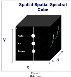
Figure 1

Data Space

Understanding the Data Space

Based on the project development undertaken by

Hornak and Servoss, it was known that the spatial-spatial-spectral information from a phantom could be imaged using the backprojection of several MRI scans. To understand how the backprojection can be applied in this case, it may be helpful to think of a cube in the three-dimensional spatial, spatial, and spectral space discussed earlier, [x,y,δ] respectively. This cube represent the real location of a plane, [x,y] of materials that have some recordable depth of spectral information, δ. This spectral information corresponds to a term

referred to as the chemical shift of a substance. The backprojection attempts to reconstruct this representative cube.

The Concept of Projections

The backprojection assumes that a circle inscribes the edges of the cube such that it is aligned normal to the y-axis and centered at the center of this imaginary cube. The data contained in the cube is 'seen' by the imager as if the spectral and spatial information were 'projected' onto a plane located tanget to the circle.

Specifically, for the purposes of this application, it was assumed that data was collected in projected planes [y,δ] located at equally spaced interval angles of θ around half of the circle. Therefore, each of these intervals is refered to as the projection through the associated angle, θ. The backprojection algorithm implemented used the inverse of a standard Riemann sum, as discussed in the IDL programming library. The conditions for the collection of each of these projections was introduced by P.C. Lauterbur and further developed by

(11)

Here, θ is the current selected projection angle around the unit circle, BW_θ=0 is the bandwidth at zero degrees

and BW_θ₌₉₀

is the bandwidth used to attain the ±90° projections. The actual ability of the MR imager to produce an image at a scan angle of 90° is limited by the impossibility of producing an infinite magnetic gradient, G. This is better explained by the expression of projection angles as defined by spectral width, θ, spatial width, D and the gyromagnetic ratio γas in Eq. 3.

(3) θ = tan-1(γGD/θ)

Limitations and Artifacts of the Procedure

From Eq.3 we can appreciate the impossibility of attaining a projection angle equal to 90°, because the G_max must be some finite value. According the the equation, only an infinite gradient could produce a sample at 90°. To achieve this projection, this limiting angle was reconstructed using an interpolation technique. This is one reason for interest in characterizing the achievable resolution of the imaging technique.

The other area for concern stems directly from the manner in which the data is reconstructed during the backprojection. Ideally, if the projections were continuous from 0° to 360°, the [x,y,δ] cube could be reconstructed perfectly. However, the projections are recorded at discrete intervals of angle. Before

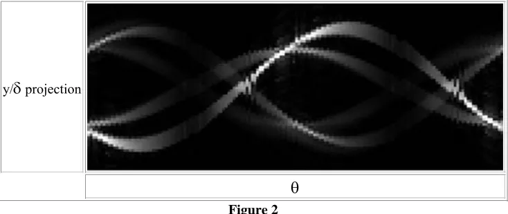
backprojection takes place, all of these discrete projections are ordered from 0° to 360°, the projections in the interval 180° to 360° are inverted ordering of the previous 0° to 180° projections. (When these ordered projections are displayed edge-on, the profile appears sinusoidal. For this reason, the ordered set of

[image:11.612.123.490.417.572.2]

projections is referred to as the sinogram.) Because of this, the question becomes one of the success of the approximation. How many projections, each requiring a MRI scan of some real time, effectively resolve the [x,y,δ] image when omitted projections are interroplated?

Figure 2

Sinogram of assembled projections of the spatial-spectral space as a function of projection angle

y/δ projection

θ

Table of Contents

Methods

(12)

number of projections used was reduced. The task, therefore, became to observe the change in abilty to

resolve a set of [x,y,δ] data as fewer and fewer projections were included in the creation of the sinogram. The metric selected for this characterization was point-spread measurements. To test for this effect, a phantom having known spatial and spectral characteristics was constructed as the resolution target.

Phantom Construction

Using earlier MR data collected by Hornak and Servoss as a guide, the phantom target was constructed. The phantom consisted of three ten centimeter MR glass test tubes aligned parallel and vertical in a cylinder filled with suspension of conducting material. Each of these test tubes had a width of seven millimeters. Alignment of the test tubes was crucial because the tomographic process of MR imaging selects a plane of some

thickness. It was necessary to know that in the selection plane the tubes could be seen as regular cylinders. This allowed the bulk of each cylindrical section to be summed to a single circle with complete overlap of area for the entire section of test tube. The surrounding suspension was selected to reduce noise from the sample area. Each test tube was filled with one of the following: water, decane, and a water-decane solution. The concentration of each of these liquids was selected to produce T1 times of nearly the same magnitude3.

This precaution was taken to ensure that, when imaged, the peak spectral response of all of the phantom materials would be scaled to similar intensities. This precaution was taken to attempt to keep the effects of noise on signal intensity as uniform as possible for each signal peak.

Data Collection

This phantom was imaged using the MRI at Strong Memorial Hospital. The tubes were placed and secured in the imager, any vibration or misalignment could nullify several hours of image collection. Again, care was taken to ensure the alignment of the test tubes was maintained. The objective, observing the change in resolution as a function of projection angles in the spatial-spatial-spectral MRI procedure, demanded that a high number of projections be collected. Previous experiments had determined that as many as 80 regularly spaced projections could be collected in about five hours. To assure that these projections were recorded at the correct intervals, the spreadsheet model predicted parameters for the bandwidth, BW(θ), and

phase-encoding gradient, G, as a function of projection angle.

Sinogram Construction

The images of the 80 projections were ordered by respective angle and constructed into the sinogram of 160 angles. The backprojection of this sinogram was decided by convention to represent the for maximum resolution possible for bench-marking purposes. To simulate a backprojection constructed from fewer

projections, samples were omitted from the sinogram at this step. An integer value, n, of projections could be specified to be skipped from the sinogram when the backprojection was implemented. This value was

incremented from 1 to 27. For each progressively fewer number of projections used, the spectral profile of the center segment through the phantom was recorded as a [y,δ] image.

(13)

projection densities of the sinogram used. In order for this metric to be applied, peaks needed to be located in the high resolution, bench-mark image.

Local maxima were used to determine peaks. First, an averaging kernal was applied to the image to reduce insignificant noise that is typically magnified when calculating derivatives. Then, a simple derivative was applied in the y-dimension4. This returned several points that were checked for local maxima using the second derivative test. A similar calculation was performed in the δ-dimension, but points that were not coincident with peaks detected in the y-dimension were rejected. This assumption was made based on the knowledge that spectral peaks detected outside the spatial peaks did not lie within the test tubes and must therefore be noise. Peaks were thereby assigned to four locations where both spatial and spectral peaks were coincident. Because images from the backprojections were expanded from 64 pixels to 512 image pixels, all image processing performed assumed a pixel width of eight image pixels.

In this application, the minimum value in any image was not always zero. Because of this, the width at half height was defined for each individual dimensional segment. Each image is a series of spatial columns and spectral rows, any of which could be manipulated as a 1-D array. For any peak point, the spatial width at half maximum at that point was determined by setting the floor of the particular spatial column to the minimum of that vector. The maximum for each peak was measured from this new base value. The same standard was maintained for determining the peak heights when calculating the spectral width at half maximum, with the consideration that the vector of interest in these cases was in of the current spectral row.

Determining Point-Spread

The point-spread in either the spatial or spectral dimension was then calculated as the difference in the real pixel FWHM at a point in any image to the real FWHM of the bench-mark image.

Table of Contents

Results

Image Attributes

Some conceptual difficulty may be encountered when examining the images produced by this imaging technique. When approaching these results, it may be helpful for one to note that each image is a two

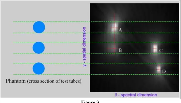
dimensional slice from the three dimensional [x, y, δ] space. The slices were taken through the center of the test tubes in the [y, δ] plane and appear in Figure 1 as the vericle line through the test tubes. This plane was selected for all observations because it contained both spatial and spectral information from each of the three test tubes. Figure 3 shows the relationship of the phantom and the spatial-spectral image. The spatial extent in the y dimension of each test tube is represented by the breadth between the dashed green lines. Spectral data is expressed along the horizontal δ

axis. The actual content of the images is contained in the monochrome brightness values. Larger signal responses are represented by higher brightness values in the image.

(14)

detected diameter of the phantom tubes. The horizontal width of each peak indicates ranges of highest

frequency response to the phantom. Each of the peaks are labeled alphabetically. Peak 'A' is aligned with the test tube that was filled with water. Peaks 'B' and 'C' are both responses detected from the test tube filled with the reverse micelle solution. This solution was a combination of both water and decane. Peak 'D'

[image:14.612.125.489.103.311.2]

corresponded to the response from the tube filled only with decane.

Figure 3

Bench-mark resolution spatial-spectral image (constructed with 80 projections)

Presentation of Results

The point-spread of each point was calculated in both the spatial and spectral direction. Point-spread is reported here as the FWHM in real pixel values as a function of θs; the number of projections from the

sinogram used to reconstruct the data. In order to illustrate the extent of these point-spreads, the FWHM has been traced on all the images as red lines, which appear in the images as a set of cross-hairs.

A total of 27 images were constructed and evaluated. The appendix contains links to each of these images. The images are ordered according to an index value 'n'. This value indicates that each image is composed of 100%/n of the available 160 θ_s.

The point-spread as a function of n is charted for the spatial and spectral widths of all the points. The abscissa is labeled in values of projections used and collection time. The projection values appear in red,

corresponding to the red of the cross-hairs. Because part of the objective was to relate achievable resolution to clinical data collection time, the value of θs

(15)

Peak A

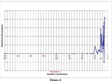
[image:15.612.125.488.111.375.2]

At the highest resolution, this peak is the brightest. This quality makes this signal easiest to detect against the contrast of any possible noise. The spectral response of the material in this tube corresponds to water. The ability to resolve the spatial extent, corresponding to the width of the test tube, is maintained when using as few as θ_s = 26. The spatial point-spread at this resolution is 4 real pixels.

Figure 4

Spatial Point-Spread as a function of number of projections and imaging time for water-filled test tube

The spectral point-spread for peak A is well behaved and does not vary until the image constructed from the

θ_s = 32. At this resolution, the point-spread is only 1 real pixel. This deviation of 1 is maintained until at only

(16)

[image:16.612.125.487.42.283.2]

Figure 5

Spectral Point-Spread as a function of number of projections and imaging time for water-filled test tube

Peak B

The signal from peak B varies the most over the range of projections used. Of all observed peaks, peak B varies in point-spread for the range of θs

used. This peak is the response from the water component of the reverse micelle solution. Peak B and peak A lie at the same spectral coordinate. For this reason, the illustrated width of peak B is sometimes obscured by the illustration of the width of peak A. Although the results of the point-spread for peak B would suggest that at least 80 projections would be needed to reproduce the most acceptable determinate of the spatial extent of a phantom, there may be some bleed effect from similar materials in close proximity that would be cause for review. Using θ_s

(17)

[image:17.612.125.488.44.279.2]

Figure 6

Spatial Point-Spread as a function of number of projections and imaging time for water component of the reverse micelle test tube

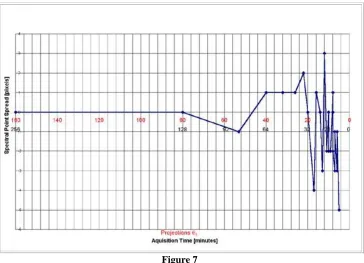
The spectral point-spread remains zero for only one lower set of sinogram projections than that of the spatial resolution. This result suggest that θs

must be at least 54 to produce a point-spread of zero. As in the case of the spectral resolution of peak A, the point-spread does not increase beyond 1 pixel until as few as 22 sinogram projections are used.

Figure 7

[image:17.612.125.489.411.674.2]

(18)

Peak C

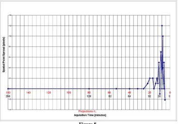
As in the case of peak A, the point-spread of the spatial resolution is very well behaved. This signal is the response of the decane component of the reverse miscelle solution in the phantom. Peak C has a spatial point-spread that does not vary until as few as 22 projections from the sinogram are used for image

[image:18.612.124.491.126.383.2]

reconstruction. At this threshold, the point-spread is only 1 pixel. This value quickly jumps to 2 pixels at the 20 projections level.

Figure 8

Spatial Point-Spread as a function of number of projections and imaging time for decane component of the reverse micelle test tube

Peak C has a spectral point-spread that varies to 1 pixel as soon as the θs = 80 image. This variance is not

(19)

[image:19.612.126.487.42.277.2]

Figure 9

Spectral Point-Spread as a function of number of projections and imaging time for decane component of the reverse micelle test tube

Peak D

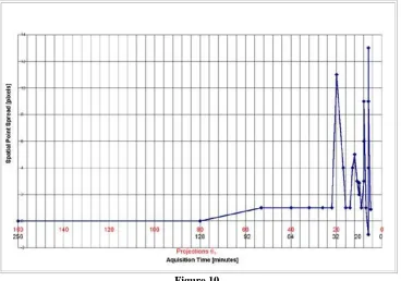
Peak D is the result of the signal detected from the decane test tube in the phantom. The spatial point-spread remains zero or 1 up to the 22 projections level. When as few as 20 sinogram projections are used for the reconstruction of the image data at this location, the point-spread increases to 2 real pixels.

Figure 10

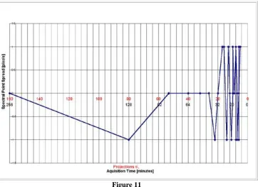
[image:19.612.124.492.425.683.2]

(20)

[image:20.612.127.489.60.322.2]

The spectral point-spread of peak D never exceeds 1 pixel. However, this deviation is detected as early as the image created using θs = 80.

Figure 11

Spectral Point-Spread as a function of number of projections and imaging time for the decane-filled test tube

Table of Contents

Discussion

(21)

[image:21.612.355.571.41.222.2]

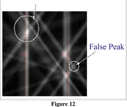
Figure 12

Artifacts of the spatial-spectral imaging process

There remain plenty of instances for interpretation of results for the specific needs of an application, yet the data would suggest - at least to the order of spectral amplitudes and spatial separations used here - that a point-spread of 2 real pixels can be overcome by using θs = 80. Such a decision must also consider sources of

error, the tolerances needed for an application, and the time available for the implementation of the procedure.

Sources of Error

The images and the information they contain are the results of an imaging system that relies on an extensive amount of digital processing for the implementation of the backprojections. There are several locations in this procedure that errors in the construction of the images may have occurred. Such errors are artifacts of the truncation and rounding of calculations and constants used. Other possible instances of such errors may be due to assumptions made in other areas of the backprojection procedure as implemented by IDL. This may have introduced error if the transition between data on consecutive images were non linear transitions. It is also interesting to note that as the number of projections used is incremented down, the corresponding series of images seems to exhibit a rotating star pattern about peaks. To observe this effect, please see the included images in the appendix. The streaks of the star pattern are the artifact of the backprojection. Simply, these streaks would be minimized if more projections were available to the backprojection. As the algorithm stands, these lengths of brightness intersect at some points and generate new peaks that do not relate to real image information. These ghost image peaks were ignored for the application of point-spread determination, but at few projections, these artifacts may be detected as real information. Perhaps as an additional effect of the undersampling, the peaks that were expected at a certain location were occasionally shifted in either the spatial, the spectral, or both directions. A shift of a peak would produce anomalous results because the height of the peak is then taken at some location other than the maximum of the signal.

Table of Contents

Conclusions

(22)

resolution at a point-spread tolerance of 2 pixels in either dimension when using as few as 80 projections from the sinogram. This level was determined to be the lowest common denominator for both the spectral and spatial resolution at each of the four selected peaks. The results of this research suggest that a reasonable level of resolution could be attained, therefore, in as little as 40 MRI scans. The time associated with attaining this minimum level of acceptable resolution is 2 hour 40 minutes, for an average sample rate of one scan per four minutes using a generic spin echo sequence with TR=1000/TE=35ms.

The applications of such a technique could be adjusted and enhanced to achieve the same results in fewer samples. Such adjustments may include filtering, preprocessing, or some calibration method. One

improvement that the results of this research suggests is that the effects of the star pattern and smearing could be reduced in the spatial dimension by observing that areas of minimum signal in this dimension should have corresponding minimum spectral returns. In this sense, the results of the backprojection could be extruded through the spatial-spatial image by relative signal intensity for each location.

(23)

Kenneth Michel Brodeur

References

T.G. Servoss, J.P. Hornak, "Spatial-Spatial-Spectral imaging on a clinical magnetic

resonance imager."

ENC

, Asilomar, CA 2000.

1.

P.C. Lauterbur, D.N. Levin, and R.B. Marr,

Journal of Magnetic Resonance Imaging

59:536

(1984).

2.

J.P. Hornak,

The Basics of MRI, A hypertext book on magnetic resonance imaging.

http://www.cis.rit.edu/htbooks/mri/

3.

Castleman, K. R.,

Digital Image Processing

, Prentice-Hall Inc., Upper Saddle River, New

Jersey, USA, pp. 368-373 (1996).

4.

(24)

List of Symbols

Symbol Discription

ν

frequency

γ

gyromagnetic ratio

B₀ standing magnetic field

x spatial coordinate

y spatial coordinate

ν

0 Larmor Frequency, frequency of induced nuclear magnitic spin

Gx frequency encoding gradient, magnetic field gradient in x dimension

G0 phase-encoding gradient, magnetic field gradient at 0° of projection

δ

spectral frequency response coordinate: chemical shift

θ

projection angle

BW(

θ

) sampling frequency bandwidth used by MRI to record a specified projection angle,

θ

BW

θ

=0 sampling bandwidth at 0°

BW

θ

=90 sampling bandwidth at 90°

θ

spectral width of the field of view of the purely spectral projection

θ

D spatial width of the field of view of the purely spatial projection

θ

T1 spin lattice relaxation time

FWHM full width at half maximum

(25)

Characterizing Spatial-Spatial-Spectral MRI

Appendix

PDF of

Table of MRI Settings for Data Collection

Index of spatial-spectral images,

index value 'n' corresponds to the 100%/n of the sinogram used

1 2 3 4 5 6

7 8 9 10 11 12

13 14 15 16 17 18

19 20 21 22 23 24

25 26 27

(26)

(27)

(28)

(29)

(30)

(31)

(32)

(33)

(34)

(35)

(36)

(37)

(38)

(39)

(40)

(41)

(42)

(43)

(44)

(45)

(46)

(47)

(48)

(49)

(50)

(51)

(52)

(53)

(54)

(55)

(56)

Theses

Thesis/Dissertation Collections