Development and Applications of Multi-layered
Genetic Algorithms to Multi-dimensional
Optimisation Problems
by
Galina Vladislavovna Kelareva
Submitted in fulfilment of the requirements
for the Degree
of Doctor of Philosophy
University of Tasmania
Australia
Statement of Originality
I hereby declare that this submission is my own work, that no part of this thesis has be.en accepted or presented for an award of any degree or diploma by the University or any institution, and that to the best of my knowledge, this thesis contains no material previously published or written by another person except where due acknowledgment has been made in the text or in the bibliography.
Galina V. Kelareva
;c.
02.0?.
Statement of Authority of Access
This thesis may be made available for loan and limited copying in accordance with the Copyright Act 1968.
Abstract
Genetic algorithms represent a global optimisation method, imitating the principles of natural evolution: selection and survival of the fittest. Genetic algorithms operate on a randomly initialised population of potential solutions to a problem. The solutions develop by passing valuable genetic information to succeeding generations.
Genetic algorithms are known as a robust technique suitable for a variety of optimisation problems. However, when applied to complex combinatorial problems with multiple parameters, conventional genetic algorithms are usually slow and ineffective due to _the large search space.
This thesis proposes a novel approach to the development of a genetic algorithm and applies this approach to a maintenance scheduling problem in a power generation system. Problem specific knowledge is utilised to divide the problem into several layers, with each layer representing a part of the initial problem. Solutions are progressively developed, with each layer algorithm finding partial solutions that satisfy specified criteria. These partial solutions are then used as building blocks in the next layer, to progressively build up complete solutions.
The resulting multi-layered genetic algorithm is able to concentrate its search efforts in areas where good quality solutions are likely to be present, therefore producing better results than traditional genetic algorithms. Further developments of the multi-layered genetic algorithm are also suggested in this thesis. The algorithm is combined with a local search method, and heuristic rules are used for initialisation of the population. The combined method results in an effective and fast exploration of the problem's search space and is suitable for a variety of optimisation problems.
Acknowledgements
Contents
Page
Dedication ... iii
Statement of Originality ... v
Statement of Authority of Access ... v
Abstract ... vi
Acknowledgements ... viii
Contents ... ix
List of Figures ... xiii
List of Tables ... xiv
List of Notations and Abbreviations ... xvi
List of Publications ... xviii
0.0 PREFACE ... XIX 1 OVERVIEW OF GENETIC ALGORITHMS ... 1-38 1.0 Introduction ... 2
1.1 Genetic algorithms as an optimisation method ... 2-5 1.2 An exampl~ of GA optimisation ... 5-12 1.2.1 Representation ... 5
1.2.2 GA implementation ... 9
1.2.3 Results ... 12
1.3 Theoretical foundations of GAs ... 13-16 1.3.1 Holland's GA ... 13
1.3.2 Schema Theorem ... 14
1.4 Parameters and variations of GAs ... 17-37 1.4.1 Selection ... 17
1.4.2 Representation ... 22
1.4.3 Mutation ... 25
1.4.4 Recombination ... 28
2 TRADITIONAL GA
FOR MAINTENANCE SCHEDULING OPTIMISATION ... 39-74
2.0 Introduction ... 40
2.1 Scheduling as an optimisation problem ... 40-41 2.2 Case study: maintenance scheduling in a power system ... 41-45 2.2.1 Problem specification ... 42
2.2.2 Input data ... 44
2.3 Existing GA techniques for representation of scheduling problems ... 45-51 2.3.1 Indirect representation ... 46
2.3.2 Direct representation ... 49
2.4 Representation of a problem domain for maintenance scheduling ... 52-72 2.4.1 Maintenance scheduling as a representation problem ... 52
2.4.2 Indirect representation of maintenance scheduling ... 56
2.4.3 Direct representation of maintenance scheduling ... 63
2.4.4 Comparison of indirect and direct representation methods ... 69
2.5 Conclusion ... 73-74 3 MULTI-LAYERED GENETIC ALGORITHM ....•..•..•••••..••...•... 75-120 3.0 Introduction ... 76
3.1 Effective search strategies for a large problem domain ... 76-79 3.2 What is a multi-layered genetic algorithm? ... 80-87 3.2.1 Separability of a problem ... 80
3.2.2 Introducing a multi-layered genetic algorithm ... 81
3.2.3 Specifics of an MLGA search ... 82
3.2.4 MLGA parameters ... 84
3.3 MLGA implementation ... 87-99 3.3.1 Unit groupings for an MLGA ... 87
3.3.2 Interchangeable chromosomes ... 92
3.3.3 Unit convergence ... 93
3.3.4 Termination criteria ... 94
3.3.5 Pseudo-code for an MLGA ... 95
3.3.6 Increase in the population size for better peiformance ... 97
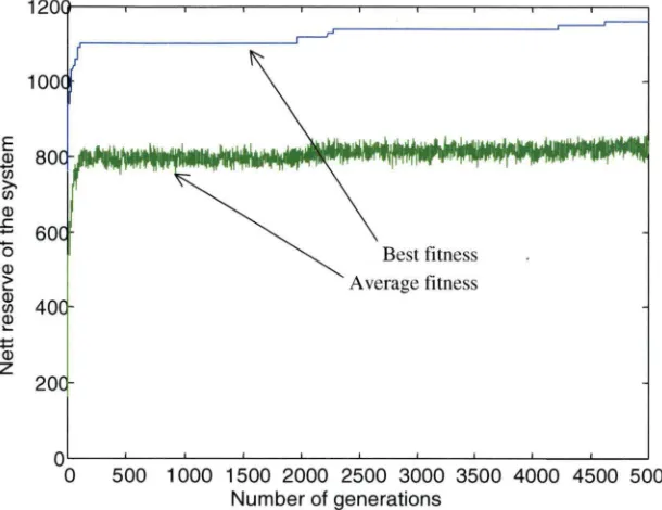
3.4 Preliminary results ... 100-103 3.4.1 Peiformance graphs ... 100
3.4.2 Evaluation of the 12-layer MLGA. ... 101
3.5 Modified gene pool criterion ... 103-110 3.5.1 Additional evaluation of gene pool candidates ... 103
3.5.2 Modifiedfitnessfunction ... 105
3.5.3 Effect of the modified pool criterion on MLGA peiformance ... 105
3.5.4 Evaluation of the 12-layer MLGA with modified pool criterion ... 108
3.6 Second example of unit groupings ... 110-116 3.6.1 A9-layerMLGA ... 110
3.6.2 Evaluation of the 9-layer MLGA ... 112
4 MULTI-LAYER GENETIC LOCAL SEARCH ... 121-157
4.0 lntroduction ... 122
4.1 Genetic local search (GLS) ... 122-124 4.2 Multi-layered GLS for a maintenance scheduling problem ... 125-136 4.2.1 Definition of a neighbourhood ... 126
4.2.2 Definition of a neighbourhood made suitable for an MLGA layer ... 130
4.2.3 Evaluation of a neighbourhood ... 131
4.2.4 Gene pool modification for neighbourhood exploration ... 132
4.2.5 Choosing the GLS parameters ... 133
4.3 Tuning the GLS parameters ... 137-148 4.3.l Layering units for an MLGLS ... 131
4.3.2 Possible parameters values ... 139
4.3.3 Gene pools and other MLGLS parameters ... 140
4.3.4 Experimantal results ... 141
4.3.5 Recommended GLS parameters ... 148
4.4 MLGLS performance ... 149-155 4.4.1 MLGLS implementation ... 149
4.4.2 Layered results for the MLGLS ... 150
· 4.4.3 MLGLS peiformance with various retained reserves ... 154
4.5 Conclusion ... 155-157 5 GREEDY MULTI-LAYER GENETIC LOCAL SEARCH WITH AN EXPANDING GENE POOL ... 159-187 5.0 Introduction ... 160
5 .1 Further improvement of the MLGLS algorithm ... 160-168 5.1.1 MLGLS with an expanding gene pool and a restricted elite ... 161
5.1.2 Greedy MLGLS ... 163
5.1.3 Local search through the entire population ... 164
5.1.4 Peiformance of the greedy MLGLS ... 164
5.2 Implementation of the greedy MLGLS ... 168-175 5.2.1 Maintaining the age diversity in the population ... 168
5.2.2 Weeding interchangeable sub-schedules from the gene pool ... 169
5.2.3 Termination criteria ... 171
5 .3 Greedy MLGLS preliminary results ... 17 5-177 5 .4 Population initialisation with a schedule builder ... 177-185 5.4.1 Combining two types of representation in one algorithm ... 111
5.4.2 The effect of the combined representation on greedy MLGLS peiformance ... 179
5.5 Conclusion ... 186-187 6 RESERCH RESULTS AND SUMMARY ... 189-194 6.1 Reserch results ... 190
6.2 Software development ... 192
6.3 Further research ... 193
7 APPENDICES ... 195-267
A.1 Gene pools for direct representation ... 195
A.2 Performance graphs for a 12-layer MLGA ... 203
A.3 Layered results for a 12-layer MLGA ... 211
A.4 Layered results for a 9-layer MLGA ... 223
A.5 GLS parameters ... 235
A.6 Layered results for MLGLS ... 245
A.7 Layered results for a greedy MLGLS ... 253
A.8 Layered results for a greedy MLGLS with heuristic initialisation ... 261
List of Figures
Figure 1.1 Pseudo-code for converting binary into Gray code ... 6
Figure 1.2 Pseudo-code for converting Gray code into binary ... 6
Figure 1.3 Pseudo-code for a traditional GA ... 7
Figure 1.4 Initial population ... 8
Figure 1.5 GA population at the end of the run (20 generations) ... 12
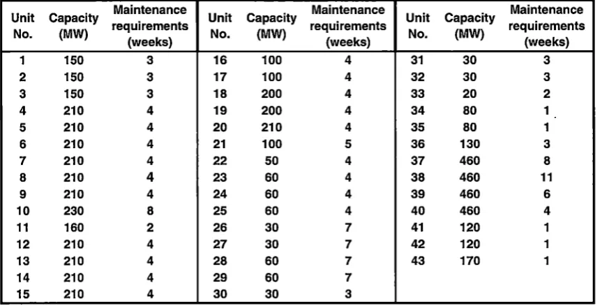
Figure 2.1 Schedule builder 'deepest first' ... 57
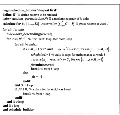
Figure 2.2 Schedule builder 'first available' ... 58
Figure 2.3 Performance of a traditional GA ... 68
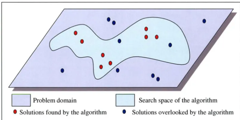
Figure 3.1 Search space of a GA with a schedule builder ... 82
Figure 3 .2 Search by an MLGA ... 83
Figure 3.3 Pseudo code for an MLGA ... 96
Figure 3.4 Example of GA performance with population size 300, pool size 300 ... 99
Figure 3.5 Performance of a GA with gene pool Criterion 3.2 ... 106
Figure 3.6 Growth of individuals in the pool during the first few generations ... 107
Figure 4.1 Pseudo-code for a GLS ... 124
Figure 4.2 Eucledean and maximum difference neighbourhoods with radius 3 ... 127
Figure 4.3 Gene pools with and without empty spaces ... 128
Figure 4.4 Neighbourhood in a circular gene pool ... 129
Figure 4.5 Neighbourhood definition with various Ne ... 135
Figure 5 .1 Age management procedure ... 162
Figure 5.2 Gene pool growth in the first layer. ... 165
Figure 5.3 Gene pool growth in the second layer ... 166
Figure 5 .4 Gene pool growth in the fourth layer ... 168
Figure 5.5 Algorithm for weeding duplicates ... 170
Figure 5.6 The greedy MLGLS performance with
T..
=15 ... 172Figure 5.7 The greedy MLGLS performance with
'T..
=55 ... 173List of Tables
Table 1.1 Binary and Gray codes for some numbers ... 7
Table 1.2 Chromosomes in the initial population ... 8
Table 1.3 Roulette wheel selection ... 10
Table 1.4 Results of crossover and mutation ... 11
Table 1.5 Population obtained after the first generation ... 11
Table 1.6 Population at the end of 20 generations ... 12
Table 2.1 Capacity and maintenance requirements of the units ... .44
Table 2.2 Predicted maximum load and gross reserve of the system ... .45
Table 2.3 Initial population with 'strict' schedule builders ... 59
Table 2.4 Initial population with 'soft' schedule builders ... 60
Table 2.5 GA performance with the indirect representation ... 61
Table 2.6 GA performance with the indirect representation and growing elite ... 62
Table 2.7 GA performance with direct representation over 300 generations ... 67
Table 2.8 GA performance with direct representation over 5,000 generations ... 67
Table 2.9 Seeded GA performance with direct representation ... 69
Table 3.1 Unit data ... 88
Table 3.2 Results of the partial GA experiments ... 90
Table 3.3 12-layer MLGA ... 91
Table 3.4 Effect of the increase in the population size on MLGA performance ... 98
Table 3.5 Performance of the 12-layer MLGA with different gene pool criteria ... 108
Table 3.6 First layers in an MLGA ... 111
Table 3.7 Last layers in an MLGA ... 112
Table 3.8 9-layer MLGA ... 112
Table 3.9 Performance of the 9-layer MLGA with different gene pool criteria ... 114
Table 3.10 Summary of the MLGA performance ... 115
Table 3 .11 Comparison of different algorithms performance ... 117
Table 4.1 Neighbourhood size and properties depending on r and Ne ... 136
Table 4.3 GLS parameters ... 139
Table 4.4 GLSa and GLSb best results in the first layer ... 144
Table 4.5 GLSa and GLSb best results in the second layer. ... 145
Table 4.6 GLSa and GLSb best results in the third layer ... 146
Table 4.7 Optimal GLS parameters ... 148
Table 4.8 Layered data from an MLGLSb run ... 151
Table 4.9 MLGLS performance with different number of layers ... 154
Table 5.1 Performance data for the first layer of a greedy MLGLS ... 165
Table 5.2 Greedy MLGLS performance ... 176
Table 5.3 Comparison of the two greedy 9-layer algorithms with R0=1240 ... 181
Table 5.4 Greedy MLGLS comparison ... 183
List of Notations and Abbreviations
T - time intervals, i = 1, ... , T N - number of units, j
=
1, ... , NC1 - capacity of unitj
M 1 - number of weeks required for maintenance of unit j N
S =
L
C1 - installed capacity of the system J=IP,
-
predicted load ip week iG, = S -
P,
-
gross reserve in week i J, -units scheduled in week iR,
=
G, -L
C1 - nett reserve in week i JE]1R0 - retained reserve parameter
a
= (
a1, a2 , ••• , aN) -chromosome with N genesA
1 - gene pool for gene j , a 1 EA
1fi
0b1
=
min { R,1Ii=
1, ... , T} -objective function of individual lF;
-
fitness of individual lR0
- retained reserve parameter K - number of layers, k = 1, ... , K
J(k) - units in layer k
N(k) - number of units in layer k
s = ( a1, a2 , ••• ,
am)
-
sub-schedule with m unitsm
L1
=
L
C1Xv - additional load on the systemJ=I
{1, if jE ]1
S(k) - gene pool containing sub-schedules found in layer k
(k) - ( (k-i)) A (k-i) 5(k-i) b h d 1 I f 1 k 1
s1 - aP .. .,aN<ll•s , a1 E 1 , s E - su -sc e u e rom ayer >
7;,
Tz,
~-
termination criteriat - generation
P ( t) - population at generation t
p E P (
t)
-
indi victual from the population P (t)
F (t)
-
fitness of the population at generationt
Ng - number of genes in an individualNe -number of changing genes in an individual
Ns -number of neighbours sampled during local search
N,Nc
(
x) -neighbourhood of x with radius rand Ne changing genesGA - genetic algorithm
PMX -partially matched crossover TSP - travelling salesman problem JSSP - job shop scheduling problem MLGA- multi-layered genetic algorithm LS - local search
GLS - genetic local search
List of Publications
1 Kelareva, G., Negnevitsky, M., "Multi-layered genetic algorithms for maintenance scheduling in power systems", Proc. Of the 2nd IASTED lnt. Conf. On Power and Energy Systems, (Crete, Greece, June 2002), pp 32-37.
2 Kelareva, G., Negnevitsky, M., "Multi-layered genetic algorithm for maintenance scheduling with multiple parameters", Australian Journal of Intelligent Information Processing Systems, Vol.7, No.3/4, 2001, pp. 122-131.
3 Kelareva G., Negnevitsky M., "Multi-layered genetic algorithm for maintenance schedule optimisation", Proc. Australasian Universities Power Engineering Conf. (AUPEC, Perth, WA, Australia, 2001), pp 379-384.
4 Negnevitsky, M., Kelareva, G., "Genetic algorithms application to scheduling problems in power systems", Proc. Of the 1 st Japanese-Australian Joint Seminar on Applications of Electromagnetic Phenomena in Electrical and Mechanical Systems (Adelaide, Australia, March 2000), pp. 123-129.
5 Negnevitsky, M., Kelareva, G., "Maintenance scheduling in power systems using genetic algorithms", Proc. Of International Conference on Electric Power Engineering (Budapest, Hungary, 1999), BPT99-445-16.
6 Negnevitsky, M., Kelareva, G., "Genetic algorithms for maintenance scheduling in power systems ",Proc. Of Australasian Universities Power Engineering Conference (AUPEC, Darwin, Australia, Sept. 1999), pp 184189.
7 Negnevitsky, M., Kelareva, G., "Application of genetic algorithms for maintenance scheduling in power systems ", Proc. Of 6th Int. Conf.on Neural Information Processing (ICONIP, Perth, WA, Nov. 1999), pp 447-451.
Preface
Genetic algorithms (GAs) belong to the group of optimisation methods simulating natural evolution and are applied in various areas, such as function optimisation, strategy planning, scheduling. Their undoubtable strength is the ability perform a global search in the problem domain in parallel. However, GAs are often considered as slow and inefficient when dealing with a real life optimisation problem with multiple parameters and a vast search space. Current research in GAs is concerned with finding the ways to increase the search efficiency when dealing with such problems.
This thesis proposes a new GA technique to provide an efficient optimisation method suitable for a problem with a large search space and vaguely defined constraints. As a case study, a scheduling optimisation problem in a power generating system is considered.
The thesis consists of six chapters. Chapter 1 gives an overview of GAs as an optimisation method and its parameters, with special attention paid to various representation techniques and corresponding genetic operators.
Chapter 2 describes the case study and examines the traditional GA approach to the problem with two different ways of representation, direct and indirect. As a result of discussion about advantages and shortcomings of both representations, the direct representation is selected for further study due to its ability to provide the complete coverage of the problem domain. However, as shown in Chapter 2, a traditional GA that uses a direct representation of the scheduling problem often cannot find any solutions of a good quality due to the overly large search space.
found in a layer are later used as building blocks in the subsequent layer when building new larger schedules. The MLGA gives an opportunity to explore the entire problem domain more efficiently than a traditional GA, however, the new algorithm is still rather slow.
Chapters 4 and 5 further develop the algorithm. In Chapter 4, an MLGA was combined with a local search method, which dramatically improved and fastened the search. In order to do this, the candidate considers several neighbourhood definitions and suggests the most suitable for the problem in question. Local search parameters are identified and fine-tuned in a series of experiments described in Chapter 4.
Chapter 5 further explored the idea of using the local search for a better exploration of the problem domain and has introduced a greedy MLGLS as another modification of the algorithm allowing to obtain results better than the ones from the GA with an indirect representation. The best results were obtained when a greedy MLGLS was combined with a heuristic initialisation procedure, also examined in Chapter 5. The resulting algorithm is highly efficient and fast optimisation technique suitable for a problem with a large search space. The new algorithm broadens the range of GA-solvable problems by performing a successful search in a large problem domain.
Chapter 6 presents a summary of the candidate's research and suggests some further developments.
CHAPTER 1
1.0 Introduction
This chapter presents an overview of genetic algorithms (GAs) as an optimisation method. After an outline of GAs and their place among other optimisation techniques, an example of a function optimisation by a traditional GA is given in Section 1.2 to illustrate a few basic concepts. The theoretical foundations of GAs, including the Schema Theorem are then discussed in the third section. A number of topics covering the implementation of GAs are presented in Section 1.4, including representational issues as well as variations in GA parameters and operators. Some of these topics are discussed in more detail in Chapters 2 and 3 with the emphasis being on specific aspects of their application as they apply to the case study. The chapter concludes with a short review of some specific techniques in practical GA applications, such as parallel and hybrid GAs, which have been chosen from the multitude of GA techniques due to their relevance to the method suggested in this thesis. These specific techniques will be referred to again in Chapters 3 and 4.
1.1 Genetic algorithms as an optimisation method
these methods have to restart from different points. Additionally, they rely heavily on the optimisation function being continuous and, preferably, having a derivative.
Enumerative methods use a rather simple idea: in a finite search space an algorithm examines the objective value at every point in the space. While the enumerative algorithms are straightforward and easy to understand, they may fail to solve real-life problems in an acceptable time due to the fact that the search space is too large (Haupt and Haupt, 1998).
Random searches have gained recognition in recent years as being an alternative to the traditional calculus-based techniques for complicated objective functions and/or large search spaces (Haupt and Haupt, 1998). In their pure form, when the search space is randomly sampled, they are not much more effective then the enumerative methods. However, some kind of a randomised process is used in numerous search techniques. GAs and simulated annealing are examples of more recent methods that use random choice as a part of their search process (Michalewicz, 1999).
GAs belong to a group of optimisation techniques known as evolutionary algorithms or evolutionary computation (Holland, 1975, Back and Schwefel, 1993; De Jong and Spears, 1993). All evolutionary algorithms represent probabilistic search methods based on the principles of natural evolution: selection and survival of the fittest by passing valuable genetic information down to succeeding generations. Evolutionary algorithms mostly differ in the way they represent a problem and in the choice and probability of genetic operators they use (Back and Schwefel, 1993). However, during last decade the differences between various types of evolutionary algorithms became less obvious due to the fact that in practical applications a number of techniques can be combined to the benefit of the resulting algorithm (De Jong and Spears, 1993).
As noted in (Goldberg 1989), GAs are different from traditional (derivative-based, enumerative) optimisation methods in several ways:
• GAs work not with parameters themselves but with some coding of parameters; • GAs search from a set of points, not one point;
• GAs use probabilistic transition rules, not purely deterministic rules; and
• GAs use the information from the objective function, not derivatives or other supplementary knowledge.
Outline of genetic algorithms
While a formal definition of GAs components is presented in Section 1.3, an initial outline of GAs is given here as an introduction to this technique:
• GAs imitate natural evolution and collective learning process in a population of individuals (Davis, 199la). Usually each individual represents a potential solution to a given problem in a search space of all possible solutions. When the first population is initiated, each individual is evaluated according to its performance. An evaluating function introduces a measure of quality for each individual, and therefore provides a means for comparison of individuals. Consequently, this measure gives an ability to decide if an individual is better or worse than the other members of the population. Following this evaluation better individuals are given more opportunity to reproduce (Schwefel and Rudolph, 1995).
• After recombination and mutation new individuals evolve with features from both parents and are then evaluated in their turn. The second generation is formed, possibly, with some best parents preserved. After a sufficient number of generations a population is obtained with solutions/individuals approaching the desired optimum (Radcliffe, 1997).
1.2 An example of GA optimisation
1.2.1
Representation
To illustrate the basic features of a GA, consider the following example of a function optimisation. Suppose a function F(x) = xsin(5x) is to be maximised on the interval 0 ::::; x::::; 2.5. The function has several local maxima and one global maximum equal to 1.58334545 at the point x=l.5957. A potential solution in that case could be described by a chromosome representing a point from the interval [ 0, 2.5]. Traditionally binary coding was used for representing numerical values. In this case a chromosome consisting of N genes b1b2 ••• bN, where each of the genes is either 1 or 0, would
N-1
represent a numerical value of v0 =
L
2' bN-• . If it should represent a corresponding part 1=0of an_ interval, as in our case, the numerical value is calculated by the following formula:
v=min+v0(max-min)/(2N -1) (1.1) If the number of genes in a binary chromosome is taken to be 8, the search space of the problem would consist of 28 = 256 points, or 256 parts of the given interval [ 0, 2.5]. Such representation allows the interval to be examined with a precision up to two decimal places. For example, a string 01001101 represents a numerical value of
v0 =0*27 +1*26+0*25+0*24+1*23+1*22+0*21+1*2°=77 or in our case 77th
' '
Gray coding
A direct binary representation has a disadvantage in that two adjacent values can be represented by strings that have very little in common. For example, in a binary representation with three genes the adjacent integers 3 and 4 are represented by strings 011 and 100 respectively. It is possible to avoid such discrepancy if Gray coding is used instead of binary coding. The algorithms for converting a binary number into Gray code number and back are given as pseudo-codes in Figure 1.1, while precise formulae for the standard binary and Gray decoding are given in Section 1.4.
begin Binary-to-Gray/* b=(b1, ..• ,bN)-binary number,
I* g=(gJ, ... ,gN)-Gray code number gl=b1
for i=2:N
g1=XOR(b1, b,_1)
end end
Figure 1.1 Pseudo-code for converting binary into Gray code
begin Gray-to-Binary/* b=(b1, ... ,bN)-binary number,
end
/* g=(g1, ... ,gN)-Gray code number b1=g1
for i=2:N
end
if gi=l, b1=NOT(b,_1)
else b,= bi-1
Figure 1.2 Pseudo-code for converting Gray code into binary
Table
1.1
Binary and Gray codes for some numbersDecimal Binary Gray code 0 OOO OOO
1 001 001 2 010 011 3 011 010 4 100 110 5 101 111 6 110 101 7 111 100
1.2.2
GA implementation
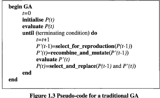
Figure 1.3 gives the pseudo-code for a traditional GA.
begin GA t=O
end
initialise P( t) evaluate P(t)
until (terminating condition) do t=t+l
end
P ' ( t-1 )=select_for_reproduction(P( t-1 )) P ' ( t )=recombine_and_mutate(P ' ( t-1 )) evaluate P'(t)
[image:25.563.111.441.346.549.2]P(t)=select_and_replace(P(t-1) and P'(t))
Figure 1.3 Pseudo-code for a traditional GA
Let us consider the operation of a GA step by step.
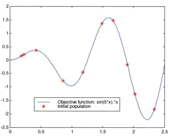
Initial population
is shown in Table 1.2 while Figurel.4 illustrates the initial population as points on the graph of the objective fu nction.
Table 1.2 Chromosomes in the initial population
Chromosome number 1 2 3 4 5 6 7 8 9 10 1.5 0.5 0 -0.5 -1 -1 .5 -2
Gray code Numerical value 11010100 1.4902 10011001 2.3333 00111110 0.4216 0 1 1 1 1 1 0 0 0.8529 00011100 0.2255 01000100 1.1765 10101001 2.0196 10100011 1.9020 1 1 1 1 1 1 1 1 1.6667 00011010 0.1 863
*
Objecti-.e function: sin(5•x).*x Initial populationObjective function value 1.3708 -1.8273 0.3622 -0.7689 0.2037 -0.4590 -1 .2593 -0.1615 1.4788 0.1495
-2.5 c__ _ _ _ ..__ _ _ _ ..__ _ _ _ ..__ _ _ _ _.__ _ _ ____,
0 0.5 1.5 2 2.5
Figure 1.4 Initial population
Elitism and selection
each generation. It means that the selection mechanism should choose 9 out of 10 individuals for reproduction while the best individual is retained as it is.
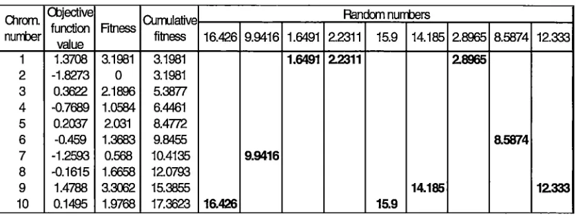
In this example one of the popular selection mechanisms, the roulette wheel selection (RWS) is used. The RWS mechanism was suggested by Holland (Holland 1975) and its idea is quite simple: each chromosome is assigned a segment of a roulette wheel proportional to its fitness. The wheel is then rotated as many times as needed for the specified number of individuals to be selected. It is obvious that some individuals can be selected many times while others will not be selected at all.
RWS provides good individuals a proportionally better chance to reproduce. Before the selection takes place, the fitness evaluation of a chromosome should be considered. In some GAs the fitness can be equal to the objective function value. In the case of RWS however the fitness values should be non-negative, yet in this example the objective function F(x) is negative in some points of the search space. Therefore some additional measure is needed to transform the objective values into fitness values suitable for RWS selection, for example, subtracting the minimal objective value from all objective values, if the former is negative. This is not necessarily the best possible way to define fitness, but sufficient for the purposes of this optimisation example. The fitness values of the initial population are given in the Table 1.3.
One of the faults of the above fitness assignment is that the chromosomes with the smallest fitness will not get any portion of the wheel if their fitness is negative or zero and, therefore, they will have no chances to reproduce. This may lead to the loss of potentially valuable genes and a population convergence to a local optimum instead of the global one.
The random numbers generated and chromosomes that were selected are given in Table 1.3. As shown in the table, chromosome #1 is selected three times, the best chromosome #9 is selected twice, as well as chromosome #10. Chromosomes # 6 and 7 are selected once each.
Table 1.3 Roulette wheel selection
Olrom. ClJjective OJrrulative Random nurrbers
nurrber function Rtness fitness value 16.426 9.9416 1.6491 2.2311 15.9 14.185 2.8965 8.5874 12.333 1 1.3708 3.1981 3.1981 1.6491 2.2311 2.8965
2 -1.8273 0 3.1981 3 0.3622 2.1896 5.3877 4 -0.7689 1.0584 6.4461 5 0.2037 2.031 8.4m
6 -0.459 1.3683 9.8455 a5874
7 -1.2593 0.568 10.4135 9.9416
8 -0.1615 1.6658 12.0793
9 1.4788 3.3062 15.3855 14.185 12.333
10 0.1495 1.9768 17.3623 16.426 15.9
Crossover and mutation
After the necessary number of individuals are selected, a new population is formed with the help of crossover and mutation operators. In a crossover, pairs of chromosomes exchange their genes after a randomly selected crossover point. The actual crossover performance is shown in Table 1.4. As chromosome #1 was selected in both the third and fourth times, the crossover does not produce any new individuals in the second pair. Since nine chromosomes were selected, one of them does not have a partner and does not participate in the crossover, although it still has a chance to mutate.
Mutation is another genetic operator which randomly changes the value of a gene. Traditionally it is considered secondary to crossover and is performed with a small mutation rate. As shown in Table 1.4, in the GA example examined in this section, just
'
Table 1.4 Results of crossover and mutation.
Chromosome Crossover Initial Crossover result Mutation result number point chromosomes
10 4 00011010 00011001 00010001 7 10101001 10101010 10101010 1 2 11010100 11010100 11010100 1 11010100 11010100 11010100 10 6 00011010 00011011 00011011
9 1 1 1 1 1 1 1 1 11111110 11111110 1 5 11010100 11010100 11010100 6 01000100 01000100 01000100 9 1 1 1 1 1 1 1 1 11111111 1 1 1 1 1 1 1 1
Note: a mutating gene is shown in bold
New population
After a new population (children, offspring, second generation) is formed, it replaces the old population less the one elite parent which is retained. The new population is shown in Table 1.5, and it is obvious that the population has improved already. There are two copies of the best individual so far, chromosomes # 1 and 10 (chromosome #1 was the elite in the original generation), while the number of individuals with a negative objective value has reduced from 5 to 2.
Table 1.5 Population obtained after the first generation
Chromosome Gray code Numerical Objective number value function value
1.2.3
Results
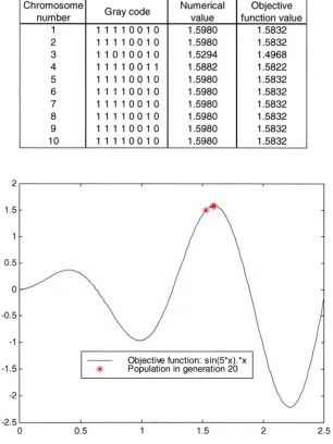
The steps that have been described, i.e. the algorithm, is repeated until some termination criterion is satisfied, for example, the maximum number of generations is reached. For this example the population after 20 generations is shown in Table 1.6 and Figure 1.5.
[image:30.562.131.437.224.632.2]1.5 0.5 0 -0.5 -1 -1.5 -2 -2.5 0
Table 1.6 Population at the end of 20 generations
Chromosome number 1 2 3 4 5 6 7 8 9 10 0.5
Numerical Objective Gray code value function value 11110010 1.5980
11110010 1.5980 11010010 1.5294 11110011 1.5882 11110010 1.5980 11110010 1.5980 11110010 1.5980 11110010 1.5980 11110010 1.5980 11110010 1.5980
Objective function: sin(5*x). *x Population in generation 20
1.5 1.5832 1.5832 1.4968 1.5822 1.5832 1.5832 1.5832 1.5832 1.5832 1.5832
2 2.5
Figure 1.5 GA population at the end of the run (20 generations)
1.3 Theoretical foundation of genetic algorithms
1.3.l
Holland's GA
A Holland's GA is a particular type of GA, with the following specific features (Holland, 1975; Schaffer et al, 1998):
• Individuals are represented as bit strings of fixed length N, that is, aE {o,1t.
• A crossover operator is used for recombination, exchanging sub-strings between randomly chosen individuals. Length and position of the sub-strings are arbitrary but identical for both strings. The crossover probability is usually taken to be from 0.6 to .95.
• The mutation operator randomly changes the bit value with the small probability of 0.01 to 0.001 per bit.
• Assuming a maximisation problem and positive fitness of individuals, a probabilistic selection operator builds the next generation from existing individuals with probabilities proportional to their fitness.
In spite of being a simple algorithm and, in many cases, with only limited possibilities, Holland's GA has received much attention from various researchers and has been thoroughly investigated from the theoretical point of view (Goldberg, 1989a; Grefenstette 1986; Schaffer et al, 1998). As a result, while many GA techniques are based on empirical results, the theoretical foundations of GAs are based on the Holland's GA analysis and, in some cases, have been developed even further to explain more sophisticated types of GAs.
1.3.2
Schema Theorem
Holland's fundamental Schema Theorem provides the theoretical base for evolutionary algorithms in general, as well as a particular GA optimisation technique. While it is referred to and described in numerous works produced by various researchers in GAs, one of the best and complete interpretations was given by N.J. Radcliffe in (1997). The following definitions are based on Radcliffe's interpretation.
Definitions
Definition 1.1 (representation, chromosome, gene, allele). Let S be a search space, that is a set of objects over which the search is to be performed. Let
Ai, ... , A.
be arbitrary finite sets with I=
Ai
x A x ... x
A.
.
Let g be a function, mapping vectors from I into the search space, that is, g : I ~ S . Then the pair (I, g) is called representation of S , I is called a representation space and g is known as a growth function.The members of the representation space are then called chromosomes, individuals or genotypes. Each x E I can be represented as x
=
(x1, x2 , ••• , xn) EAi
x Ax ... x
A.
or as a string, x1x2 ••• xn , where the components x1 are called genes. The setsA
are usuallycalled allele sets or gene pools (Radcliffe, 1997; Eshelman, 1997).
Definition 1.2 (schema). Let I=
Ai
XA
x ... xA.
be a representation space. For each allele setA
an extended setA#
is defined asA# =A
u { #}, where # is known as a 'wild card' or 'don't care' symbol. Then a schemaq
is any member of the set 8, defined as8=.Ai#xA:x ...
x~ (1.2)that is, a chromosome in which some alleles may be replaced with#.
Schemata are also known as hyperplanes and similarity templates. The members of a schema are usually referred to as instances (Radcliffe, 1997).
Definition 1.3 (fitness function). Let S be a search space, F: S ~ ffi:+ be an objective function and g : I ~ S be a growth function for the representation space I. Then any function f : I ~ ffi:+ will be called a fitness function, if the following property holds
f
(x)=
max(f) {::::} F(g(x))=
opt(F),I g(I) (1.3)
where opt is minimum, if F to be minimised and maximum if F is to be maximised.
Schema theorem
The following is Holland's Schema Theorem, as formulated by Radcliffe in (1997):
Theorem 1.1 (Schema Theorem). Let
q
be any schema over a representation space I being searched by a traditional GA using fitness-proportional selection, specified recombination and mutation operators and generational update. Let Nq(t) denote the number of instances of the schemaq
present in the population at generation t. Thenwhere ·
A
( Nq(t + 1)
I
Nq(t))~
Nq(t) l_!_(t) [l-Dc(q) ][1-Dm (q)], f(t)(A_·I
B) denotes the conditional expectation value of A given B;(1.4)
jq(t) is the observed fitness of the schema
q
at generation t, that is, the mean fitness of all chromosomes in the population that are members ofq;
f
(t) is the mean fitness of the entire population at generation t;Significance and limitations of the Schema Theorem
Most researchers agree that the Schema Theorem, though being simple and easily proved, provides the theoretical foundations for evolutionary algorithms (Goldberg, 1989a; Radcliffe, 1997; Michalewics, 1999). In particular, the theorem can be applied to GAs, if suitable bounds can be estimated for disruptiveness of the operators, which can be easily done in many cases, since most recombination operators that are used in GAs have the property of respect, that is, whenever two parents are instances of a particular schema, their offspring obtained via respectful recombination will be instances of the same schema as well (Radcliff, 1991). For example, a specific case of uniform crossover was well investigated (Syswerda, 1989; Spears and De Jong, 1991).
However, it is important to note that the Schema Theorem applies to GAs only if they use fitness-proportional selection (Radcliffe, 1997). Therefore, the theorem cannot be straightforwardly extended to selection methods that depend on the fitness of the offspring, in particular,
(µ
+
.IL)
and(µ, .IL)
selection methods used in evolution strategies (Back and Schwefel, 1993). Despite this, multiple practical applications of GAs have demonstrated that a number of different selection and recombination methods work sufficiently well even if they don't comply exactly with the restrictions of the Schema Theorem. It is debated that the most important paradigm that results from the theorem is the building block hypothesis which gives some explanation for the success of evolutionary algorithms.Building block hypothesis
Goldberg formulated a building block hypothesis as: "Short, low-order, and highly fit schemata are sampled, recombined and resampled to form strings of potentially higher fitness" and " ... a genetic algorithm seeks near optimal performance through the juxtaposition of short, low-order, high-performance schemata, or building blocks" (Goldberg 1989).
1.4 Parameters and variations of GAs
1.4.1
Selection
GAs employ two types of selection in two stages of the algorithm: selection for reproduction and selection for replacement. In each generation some individuals are chosen for reproduction, while later the old population is partly or totally replaced by offspring. In Holland's original GA, individuals were chosen randomly with probability proportional to their performance, that is, better individuals were given more chances to reproduce. Holland's proposal was that only one or two new individuals were created in each generation, and they replaced randomly chosen individuals from the old population. In other modifications of the algorithm, the number of offspring could be equal to the number of parents, replacing the old population completely.
Selection pressure and takeover time
Selection mechanisms are characterised by a parameter called selection pressure which relates to the takeover time value. This value describes the number of generations needed under pure selection (that is, without recombination and mutation) for an initial individual with the best fitness to fill the entire population (Goldberg, 1989a). If the takeover time of a selection is large it means that the selection pressure is small and vice versa. If a selection pressure is too big, the population loses diversity and converges very fast. On the other hand, a low-pressure selection operator provides mutation and recombination operators with the opportunity to perform a thorough search of the problem's domain (de la Maza and Tidor, 1993; Goldberg and Deb, 1991).
Proportional selection for reproduction
The most popular and widely used selection mechanism for reproduction is proportional selection (Back and Hoffmeister, 1991; Bramlette, 1991; Grefenstette, 1997a). Except for random selection, when individuals are chosen without any reference to their fitness, selection can be divided into three steps:
•
•
Defining an individual's probability to be selected, usually proportional to its fitness; and
Sampling the population .
Let us consider these three steps in more detail.
Fitness evaluation
The fitness function, as was mentioned in Section 1.3.2, is any function that maps the objective function into non-negative real numbers. If a proportional selection is used, the probability of an individual being chosen for reproduction is a function of its fitness. Although this type of selection is widely used, it may cause a GA to behave very differently when optimising similar functions, like y
=
ax2 and y=
ax2 + b . If the value of b is large compared to the differences in the values of the term ax2, then the probabilities for selecting the individuals in the population will be very similar and the selection pressure will be very weak.
To avoid this problem, the fitness could be scaled, that is, the fitness function is modified to adjust the selection pressure types (Grefenstette, 1986; Goldberg, 1989a). For example, a linear scaling function can be used, where the actual chromosome fitness is calculated as
f/=axf,+b,
and parameters a and b are chosen to increase the best fitness compared with the average fitness. This way the fitness of an individual is related to the average fitness and the selection pressure is increased. On the other hand, scaling may lead to dominance of a few good individuals, since if one individual is much better than the rest of the population, it will be selected for reproduction more frequently. As a result, more copies of that individual are obtained in the following generations and a GA will converge premature I y.
M-1 in a population of M. Ranking eliminates the need for fitness scaling and has proven to be an efficient method suitable for many applications (Goldberg and Deb,
1991; Grefenstette, 1997,b).
Selection probabilities
After the fitness values are assigned, a probability distribution should be defined in such a way that the probability of an individual being selected is proportional to the individual's fitness (Grefenstette, 1997,a):
p = f(x,) I N
Itcx,)
1=!
Sampling mechanisms for a proportional selection
•
The RWS technique, discussed in Section 1.2.2 is a popular sampling mechanism used in traditional GAs (Holland, 1975). The probability distribution is used to allocate a segment of the roulette wheel to each individual in the population. The wheel is then spun as many times as the number of parents to be selected, choosing one parent at a time. Such implementation may result in a high variance in the number of children assigned to different individuals, and it is possible that even the best individuals could be overlooked by this sampling and not be selected for reproduction (Grefenstette, 1997,a).Other types of selection for reproduction
There exist types of selection for reproduction other than purely proportional selection. Some of these selection mechanisms are described below.
• Another popular way of selecting individuals for reproduction is to perform a tournament selection (Goldberg and Deb, 1991), when a small subset of the population is chosen randomly and a number of best individuals from this subset are selected. The size of the subset is a parameter which defines the selection pressure. Tournament selection is not affected by scaling or transaction of a fitness function. It is less subject to dominance by a few good individuals and, consequently, premature convergence (Angeline, 1997).
• Boltzmann selection thermodynamically controls the selection pressure, usmg principles from simulated annealing (de la Maza and Tidor, 1993). The fitness function of an individual is defined as following:
f(x,)
=
exp(F(x,)/T),where F(x,) is the objective function evaluated for the
i1h
individual and T is a variable temperature parameter (Mahfoud, 1997). Boltzmann selection can be employed to indefinitely prolong the search in order to obtain better final solutions. • Disruptive selection was suggested by Kuo and Hwang in (1993) as the means toexplore extreme solutions in the population. Traditional GAs are based on either stabilising or directional selection that tend to eliminate individuals with extreme values or increase the mean value of the population, assuming a maximisation problem (Kuo and Hwang, 1993). To promote diversity in the population and help a GA to find better solutions a disruptive selection was proposed, based on a nonmonotonic fitness function. The fitness is defined as follows:
f(x)
=
IF(x)-F(t)Iwhere F(x) is the objective value of the solution x and F(t) is the mean of all solutions in the population at generation t (Kuo and Hwang, 1993). Thus, the
Selection strategies for replacement
There are a number of different replacement strategies (Eshelman, 1997). The difference in replacement selection methods could be described as the difference between (µ+A,) and (µ,A,) evolution strategies (Back et al, 1991 ). If µ parents produce A, offspring, then in (µ+A,) evolution strategies the best µ individuals for the new population are chosen from both generations (Eshelman, 1991). In (µ,-1) evolution strategies µ new individuals are chosen from A, offspring (A,>µ), replacing the parent population completely. Conventionally, the same terminology is used in GA replacement schemes (Back and Hoffmeister, 1991; Michalewicz, 1999).
Generally, the old population is not totally replaced, with at least one copy of the best individual retained for future generations. Such an approach is called elitist (De Jong, 1975; Back and Hoffmeister, 1991), and the parameter defining the proportion of the parent population to be replaced is called the generation gap (Sarma and de Jong, 1997). If the generation gap is equal to 1, the parent generation is replaced completely. Conversely, if A, in a (µ
+
A,) strategy is very small, a GA is called a steady-state GA.In an extreme case, only one child is created in a generation and the worst parent is replaced (Whitley, 1989).
Another variation in a replacement strategy which helps to sustain diversity of the pop.ulation and prevent premature convergence is that only individuals that don't have duplicates are included into the new population (Eshelman and Schaffer, 1991; Michalewicz, 1999).
1.4.2
Representation
Representation of a potential solution vector to an optimisation problem depends largely on the problem itself. The aim of the optimisation can be anything, from for example, obtaining an optimal configuration for a neuro-fuzzy expert system, modelling stalking behaviour of a predator or evasive tactics of a potential prey, to finding the shortest route connecting all given cities in a travelling salesman problem. Not only do different problems require different representation, but even the same problem could be represented in many ways and the choice of a representation type, together with the other GA parameters, could be crucial for the effectiveness of the search. Therefore, the representation of a solution is one of the most important aspects of GA implementation.
Binary strings vs real-valued vectors
A traditional Holland's GA uses binary strings of fixed length N (Schaffer et al, 1998). That is, the search space I is given as I= {O, 1r and an individual a E I is a binary
vector a= ( a1, a2 , ••• , aN) E { 0, 1} N, which is often referred to as a string a
=
a1a2 ... aN where each a1 E {0,1}. The mutation operator is then defined as a random inversion of asingle a 1 variable and the crossover operator exchanges parts of two vectors to produce offspring.
When a binary representation is used, it is necessary to define the mechanisms of
encodinganddecodingbetween the two different spaces,
{o
,1r
andffi.n.Usually thatwould mean restricting the search in whole ffi. n to the search in finite intervals
[min,, max,] for each parameterx,Effi..Inthatcase, the binary vector is divided inton
n
segments of length l, ,such that N
=
L
l, ,and then a parameterx,will be representedl=l
1-l
by a sub-string of lengthl, , (a,0+1 '...,a10+1,),where i0
=
L
11 •Thestandard binaryj=l
decodingfunction
r
'
:
{
0, lf'-7[min,, max,], according toBack (1996), is, _ . max.1-IIlln
.
, •(/-!
1J
l (al'...,a1,)-mm,+
i•
-l~
al,-J (1.5)Another way of decoding is by using the Gray code interpretation of binary strings, which often proves to be more effective since itmaps a Euclidean neighbourhood into a Hamming neighbourhood. That becomes possible due to the representation of adjacent integers by bit strings of Hamming distance one, or, in other words, the strings representing the adjacent integers differ only by one entry (Schaffer et al, 1989; Back, 1993). For theGraydecodingfunction Eq.(1.5) ischanged into
(1.6)
where ® is addition modulo two (Back, 1997).
One of the shortcomings of binary representation is thatit does not represent the entire search space, with the part it does describe only having a certain degree of precision. Despite this limitation, function optimisation remains one of the traditional areas of binary representation usage. Another area where binary representation could be successfully used is in some types of sequencing problems, such asjobshop scheduling problems(JSSP) (Nakano and Yamada, 1991; Burke and Smith, 1997). However the majority of practical applications for JSSP use real-value representation.
generalised this into the principle of minimal alphabets (Goldberg, 1989a), arguing that the requirement for binary alphabets can be omitted. This principle has been utilised in multiple practical applications (Davis, 1991a; Michalewicz, 1999) that used real-valued vectors as representation for optimisation problems.
There is no clear theoretical or even empirical justification that indicates that binary representation is the best or is suitable for any problem other than the traditional pseudo-Boolean type (Davis, 1991a; Tate and Smith, 1993; Fogel, 1997b). In fact, it has been suggested that for real-valued optimisation problems, floating-point representation proves to be more successful than the traditional binary (Michalewicz, 1999). In practical applications it has become obvious that the potential solution implementation should reflect at least some problem specific knowledge, and in some real life problems with a large number of variables it is crucial to incorporate as much additional knowledge as possible in order to get satisfactory results.
Permutations and other representations
One of the popular areas of GA applications is combinatorial optimisation problems such as the travelling salesman problem (TSP) and JSSP, in which a potential solution often can be represented as a permutation of all cities to be visited or jobs to be performed. However, in a TSP, a permutation is used to describe a cycle, therefore, a number of different individuals will represent the same solution for the problem. Moreover, such representation does not allow the use of traditional mutation and crossover operators. Many researchers have successfully used permutations as GA representation in various combinatorial problems. Goldberg and Lingle (1985) introduced the notion of ordering schemata, or a-schemata and a partially mapped crossover (PMX) operator.
Adjacency matrix representation for a TSP was suggested in (Homaifar et al, 1993). An individual is described as a binary matrix n by n, where n is the number of cities. It has 1 in an entry ( i,
j)
if there is a link between the cities i and j, and 0 otherwise. The matrix crossover is defined as an extension of a conventional one-point or two-point crossover.1.4.3
Mutation
All GAs find an optimal or near optimal solution by searching the problem space and producing variations in a given population of individuals. The mechanisms for making variations are mutation and recombination. Mutation is applied to a single parent individual, while recombination operates on two or more parents. Recombination represents a powerful exploration capability of GAs, producing new individuals by exchanging genetic information between two parents. By contrast, mutation creates new individuals by randomly modifying existing ones, thus increasing the variet;y in the population (Davis, 1991a).
Mutation can be defined as a transformation, where small random changes are made in the representation of an existing individual. If a binary representation is used, mutation simply 'flips' binary bits at random. As described by Goldberg (1989, pl4), " ... Mutation is needed because, even though reproduction and crossover effectively search and recombine extant notions, occasionally they may become overzealous and ·lose some potentially useful genetic material [ ... ]. In artificial genetic systems, the mutation operator protects against such an irrecoverable loss. [ ... ] By itself, mutation is a random walk through the string space. When used sparingly with reproduction and crossover, it is an insurance policy against premature loss of important notions."
Mutation rate
more effective (Tate and Smith, 1993). There has been a considerable amount of research into the importance of mutation in GAs and defining an optimal mutation rate (Back, 1993; Holland, 1975; Goldberg, 1989a; Grefenstette, 1986; Schaffer et al, 1998).
InGAs, themutation rate is usually takento be relatively small, being no more thanone over the string length.Incertain problems a kind of dynamic control could be beneficial, and variation of the mutation rate over the generations may accelerate optimisation (Back, 1992; Fogarty, 1989; Davis, 1989; Hesser and Manner, 1991).
Mutation inbina,.y strings
In a canonical Holland's GA, mutation operates on binary strings
N
a=(£Zi,a2,...,aN)E{0,1} of fixed lengthN (Back, 1997). Mutation consists of two
steps:
• Randomly determine positions~ ...,ik,iE{l,...,N}to undergo mutation, where
each position is selected with probability Pm ,
• Form a new string with the values at positions~ •••,ikcalculated as following:
,
-{a
1 ifu
>Pm, a, -1-ai"1f~pmwhere uE [0,1) is a uniform random variable sampled for each iE{1, ...,N} (Back et al, 1997, a).
Mutation inreal-valued vectors
Ifa chromosome is represented as a string of real integersa=(a1, a2, ...,aN)with genes
However, real valued vectors may also contain continuous parameters represented as floating point numbers. In this case mutation should be modified to make sure that its outcome is within the problem domain. For example, a non-uniform mutation is introduced to fine tune the algorithm (Michalewicz 1999).Ifa chromosome a
=
(
Gi, a2,•••,aN) is built from elements ak e [l~ uk] and an element is selected for mutation, itsnew value is determined as, {ak
+
il(t,uk-ak),ifa randomdigit is 0, a-k-ak-il(t,ak-lk), ifarandomdigitis1
where the function il(t,y)returns a value from the range [0,y]such that the value decreases whilet ,the number of the current generation, is increasing. As a result, the operator searches uniformly whentis small, that is, in the beginning of the run. The operator searches locallywhentincreases(Michalewicz, 1999).
Mutation inpermutations
Ifa problem's domain is represented as a set of permutations, it requires specific operators that produce permutations when applied to the individuals of the population. There are several mutation operators that are specifically designed for thispurpose, and many·of themare related to neighbourhood search operators.
l'here~ a number of widely used mutation operators suitable to deal with permutations:
• 2-opt operator (Lin and Kernighan, 1973) selects two points in a permutation and reverses the segment between the points. A variant of this operator reverses more than two segments at a time.
• Insert operator, which selects an element from a permutation and inserts it into a new position.Itis an operator with minimal disruption ability.
Several mutation operators were suggested in (Syswerda, 1991),
•
•
Order-based mutation also selects two elements in a permutation and swaps their positions.
Scramble mutation that randomly reorders a sublist of permutation elements, while all the other elements are left in the same positions.
There may be other mutation operators specifically designed for a particular problem.
1.4.4
Recombination
Recombination, unlike mutation, exploits the idea that if two (or more) individuals perform well, they might exchange valuable information and create a new individual (or a number of them) which may inherit the best feature of all ancestors. As it is unknown a priori what features may be contributing to good performance, the exchange is randomised. Recombination treats the specific features of individuals as building blocks and randomly combines them trying to produce better individuals. In fact, pair-wise recombination is the one feature that distinguishes a GA from other optimisation techniques, like hill-climbing or local search, even if they are population based (Eschelman and Schaffer, 1993).
Binary and integer strings recombination
Holland originally used the basic crossover operator, where two arbitrary parents swap all string bits at randomly chosen points. To illustrate the work of a simple one-point crossover, consider two individuals x and y , represented by strings of length N. If
k E { 1, 2, ... , N
-1}
is the crossover point, then the crossover operator transforms theparents x and y into two new strings by swapping the parent substrings after the position k:
X1 ••• xkxk+I ••• XN
Y1 ••• YkYk+I ••• YN
crossover X1 ••• XkYk+1 ···YN
)
It should be noted that although Holland originally applied his definition of a crossover to binary strings, crossover operators work the same way on all linear strings of different alphabet cardinality (Booker in Booker et al, 1997).
Other types of string recombination also exist. These other types include:
•
•
n-point crossover, which is a generalisation of a one-point crossover and was first implemented by De Jong (1975). The two-point crossover, when two points are chosen at random and bits of strings between the two points are exchanged is one of the most popular crossover operators, providing an effective search with minimal disruptive effect (Syswerda, 1989; Eschelman et al, 1989; Easton and Mansour, 1993).
Segmented crossover is a variant of a multi-point crossover (Eschelman et al, 1989), but instead of choosing a fixed number of crossover points, it specifies a segment switch rate which defines the probability of segments (that is, segments that are crossed over or segments that are not crossed over), ending at any point in the string. This technique provides a varying number of crossover points.
• Uniform crossover is an alternative method where parent individuals exchange randomly chosen bits (Syswerda, 1989). It uses a notion of a crossover mask rather
•
•
than points and can be beneficial in many cases. If a uniform crossover is used, it can be viewed as a form of adaptive mutation, or convergence-controlled variation (Eshelman, 1997).
Shuffle crossover, is dissimilar to traditional crossover in that it randomly shuffles the bit positions of the two parent strings before crossing them over. After the parts of strings have been exchanged, it unshuffles them. The shuffle crossover was designed " ... to eliminate the positional bias of a one-point crossover by having a schema disruption probability that is independent of schema defining length" (Eschelman et al, 1989).
Crossover rate
The crossover is controlled by the crossover rate,pcE [0, 1] , which determines the
frequency of invoking the operator.Itdepends on other GA parameters such as the population size, the choice of a selection operator, the mutation rate, etc. Commonly accepted crossover rates are Pc=0.6 (De Jong, 1975), Pc E[0.45,0.95] (Grefenstette,
1986),Pc E[0.75,0.95] (Schaffer et al, 1989). Some research shows thattechniques for
dynamically modifying crossover rate could be beneficial (Davis, 1989; Julstrom, 1995).
Recombination operators on real-valued vectors
When real-valued vectors are used as the representation of a problem's search space, a recombination operator can be defined exactly as for the linearstrings above, swapping parts of strings after a crossover point. However, other recombination operators could be introduced. Some examples of themare:
• Intermediate recombination operator, averaging components of multiple parents. According to Fogel (Booker et al, 1997), a canonical version could be defined as the follows: an offspringx'= (x;, x;, ...,x~ is the weighted average of two parents
x1=(x11,x12,•••,x1L)andx2=(x21,x22,•••,x2L),thatis
x;
=
aXi, +
(
1-a)
x
2,,for alliE {1, ...,L}where aE[0, 1] .Ifa=0.5 , the recombination operator produces a simple average of each parameter. Clearly, the operator can be defined to act on more than two parents.Inthat case it is sometimes called arithmetic crossover (Michalewicz, 1999).
• Heuristic crossover, suggested by Wright (1994), usesfitness values to determine direction of search (Michalewicz, 1999).Ifx1andx2are the two parents andx2is
not worse thanx1anduE [0, 1] ,then the single offspring is obtained as