Abstract
A new technique for predicting missing field boundaries was developed to increase the accuracy of per-field classification. This technique is based on a comparison of within-field modal land-cover proportion and local variance. Analysis was per-formed on 4-m and 20-m spatial resolution imagery derived from Compact Airborne Spectrographic Imager (CASI) data, to simulate the difference in land-cover classification accuracy between multispectral Ikonos and Satellite Pour l’Observation de la Terre (SPOT) High Resolution Visible (HRV) imagery. Ini-tially, pixel classification was performed, followed by per-field classification. The technique for detecting missing boundaries was then implemented, and per-field classification was carried out a second time using updated field boundary data. Finally, an accuracy assessment was performed. The re-sults demonstrate that classification was significantly more accurate when the missing boundary flag was used, and that simulated Ikonos imagery was considerably more accurate for this purpose than simulatedSPOT HRVimagery.
Introduction
For many years the accuracy of land-cover mapping from satellite sensors was limited by the relatively coarse spatial resolution of the imagery available (Townshend, 1992). Until the late 1990s, the finest spatial resolution imagery used widely for this purpose was that of the Satellite Pour l’Obser-vation de la Terre (SPOT) High Resolution Visible (HRV) sensor. Multispectral SPOT HRVimagery has a spatial resolution of 20 m. While this is adequate for accurate regional-scale land-cover mapping, local detail may be obscured (Fuller et al., 1994). Since September 1999, 4-m spatial resolution multi-spectral imagery has been available from the Ikonos satellite sensor. Subsequently, 3.2-m spatial resolution multispectral imagery became available from the QuickBird satellite sensor, launched in October 2001 (DigitalGlobe, URL, http://www. digitalglobe.com, last accessed 07 September 2003), and an-other spatial resolution satellite sensor, OrbView-3, is due for launch in 2003 (ORBIMAGE, personal communication, 2002). Like Ikonos, OrbView-3 will generate multispectral imagery with a spatial resolution of 4 m. This relatively fine spatial resolution has the potential to provide accurate land-cover mapping at the local scale (Aplin et al., 1997).
Traditionally, land-cover mapping from remotely sensed imagery has been performed by per-pixel classification, whereby each image pixel is associated with one or more land-cover classes (Mather, 1999). One problem associated with the use of fine spatial resolution imagery for per-pixel
Predicting Missing Field Boundaries to
Increase Per-Field Classification Accuracy
Paul Aplin and Peter M. Atkinson
land-cover classification is over-sampling, whereby the im-agery is too detailed to differentiate accurately between fea-tures of interest, instead resolving within-feature variation (Irons et al., 1985; Cushnie, 1987; Smith et al., 2002). For in-stance, where the feature of interest is a woodland area, fine spatial resolution imagery may resolve individual trees and patches of grass separating trees, leading to inaccurate per-pixel classification of woodland. Specifically, woodland pixels may be classified incorrectly as grass. The problem, viewed more generally, is that the spatial resolution is too fine relative to the level of spatial generalization desired, or speci-fied, by the user. To solve this, per-parcel (or, per-field) classi-fication may be performed whereby each field, rather than each pixel, is assigned membership to a land-cover class or classes. This removes within-field variation, thereby poten-tially increasing classification accuracy (Ortiz et al., 1997; Aplin et al., 1999a; Berberoglu and Curran, 2000).
Commonly, per-field classification is performed by inte-grating remotely sensed imagery and cartographic vector data. One major problem associated with this approach is that of missing field boundaries. Where field boundaries are missing from (or where the vectors representing them are unclosed in) the cartographic data, entire fields can be classified incor-rectly (Aplin et al., 1998). This is a particular problem when classifying large fields of rural land cover. For example, where two fields share a missing boundary, the smaller field may be misclassified in its entirety. To avoid this type of misclassifi-cation, it is necessary to identify such fields and locate miss-ing field boundaries.
This paper presents a new technique for predicting miss-ing field boundaries to increase the accuracy of subsequent per-field classification. This technique is based on a compari-son of the within-field proportion of modal land cover (the dominant land-cover class) and local variance (a descriptor of spatial variation). Such a comparison provides a simple char-acterization of the variation in land cover within each field and, therefore, an indication of the likelihood of missing boundaries. Analysis is performed on both 4-m and 20-m spa-tial resolution imagery, to estimate the difference in land-cover classification accuracy between Ikonos andSPOT HRVimagery. Initially, the methods used in this research are outlined, fol-lowed by a description of the study area and data. Then, the six-stage analytical procedure is presented, followed by some topics of discussion and, finally, five concluding points.
Methods
Four methods are described: (1) per-pixel classification, (2) per-field classification, (3) missing boundary flag, and (4) accuracy assessment.
P. Aplin is with the School of Geography, The University of Nottingham, University Park, Nottingham NG7 2RD, United Kingdom ([email protected]).
P. Atkinson is with the Department of Geography, University of Southampton, Highfield, Southampton SO17 1BJ, United Kingdom ([email protected]).
Photogrammetric Engineering & Remote Sensing Vol. 70, No. 1, January 2004, pp. 141–149.
Per-Pixel Classification
One widely used method of per-pixel classification is the maximum-likelihood (ML) algorithm, whereby pixels are as-signed to the class to which they are most likely to belong. This assignment is based on their relationship with, for each class, the mean and variance-covariance matrix characterizing the distributions of the training data in feature space (Settle and Briggs, 1987; Thomas et al., 1987; Tso and Mather, 2001).
The Mahalanobis distance Mkj(for class kat pixel loca-tionj) takes into account the variance-covariance matrix Vk
associated with a given class k: i.e., Mkj(z(xj)uk)TV
k
1(z(x
j)uk) (1)
where z(xj) is a vector of pixel values in {i1, . . . , n} wave-bands at pixel location xjand ukis the vector of means in nwavebands for class k. Using the Mahalanobis distance, it is possible to determine a predicted (Gaussian) probability den-sity for each class of interest: i.e.,
p(z(xj)k) exp[12 Mkj] (2) where p(z(xj)k) is the probability density for pixel value z(xj) as a member of class k(Thomas et al., 1987; Foody et al., 1992).
To use the above probabilities in a maximum-likelihood classification, these must be converted toa posteriori probabil-ities. Thea posterioriprobability of obtaining classkgiven pixelz(xj), L(kz(xj)) may be obtained from Bayes’ Theorem, which may be written fully to include thea priori probabili-ties: i.e.,
L(kz(xj)) (3)
where Pkis the a prioriprobability of membership in class k. MLclassification is a relatively simple and well known computational procedure available in many digital image pro-cessing systems. Despite certain drawbacks, such as the as-sumptions that the data are normally distributed and the classes to be predicted are discrete (Foody, 1996),ML classifi-cation has been used widely and has performed relatively ac-curately (Palacio-Prieto and Luna-González, 1996; San Miguel-Ayanz and Biging, 1997; Cortijo and De La Blanca, 1998; Chan et al., 2001; Frizzelle and Moody, 2001). Although alternative non-parametric classification techniques, such as artificial neural networks (Yanget al., 1999; Ji, 2000), have been shown to yield greater accuracy than theMLclassifier in certain cir-cumstances, theMLclassifier will perform accurately if the Gaussian model is appropriate.
Per-Field Classification
There are various ways in which per-field classification can be performed. It is possible to generate a per-field classification using only remotely sensed imagery by applying techniques such as edge detection or region growing to determine the field boundaries (e.g., Smith et al., 1998). Commonly, how-ever, per-field classification is performed by integrating raster remotely sensed imagery with vector cartographic data (Janssen and Molenaar, 1995; Ortiz et al., 1997; Aplin et al., 1999a), although it should be noted that error may be intro-duced where cartographic boundaries are not well matched with natural boundaries within the imagery. That is, the re-sults of such per-field classification are dependent on the accuracy of the cartographic data.
Pkp(z(xj)k)
t
r1
Prp(z(xj)r) 1
(2)n2V
k12
Per-field classification involving the integration of raster and vector data is often achieved by rasterizing cartographic data for combination with remotely sensed imagery, although it is possible to vectorize the remotely sensed imagery and integrate the image and cartographic data on a vector basis (Mattikaliet al., 1995). The remotely sensed imagery and car-tographic data may be integrated at one of three stages in the per-field classification procedure: (1) before classification (pre-classifier stratification), (2) during classification (classi-fier modification), or (3) after classification (post-classi(classi-fier sorting) (Masonet al., 1988). Most recent examples of per-field classification have employed only the latter two. For ex-ample, Westmoreland and Stow (1992), Wanget al. (1997), and Smithet al. (1997) integrate cartographic data with re-motely sensed imagery during classification to assess land-cover change on a per-field basis. Alternatively, several stud-ies have classified land cover on a per-pixel basis before integrating the classified image with cartographic data for per-field classification. The land-cover class of each per-field is pre-dicted by a statistic, such as the modal class for all pixels within that field (Janssenet al., 1990; Whiteet al., 1995; Aplinet al., 1999a). A benefit of this final approach is that it may be possible to use certain by-products of per-field classifi-cation, such as per-field modal land cover proportions (the proportion of each field occupied by the modal land-cover class) in subsequent analysis.
Missing Boundary Flag
The problem of missing field boundaries in per-field classifi-cation may be reduced by employing statistical analysis to identify fields with missing or incomplete boundaries. The procedure employed in this paper involves comparing the proportional coverage of the modal land-cover class and the local variance of each field. While the modal land-cover proportion can be extracted from per-field classification (as in-dicated above), the local variance requires further processing.
Local Variance
Local variance has been used to determine the optimal spatial resolution of remotely sensed imagery (Woodcock and Strahler, 1987; Tsang and Barnsley, 1996). Where spatial resolution is at a higher spatial frequency than land-cover variation (e.g., finer than land-cover features of interest), proximate pixel values will tend to be similar and local variance will be relatively small. As spatial resolution coarsens, proximate pixel values become less similar and local variance increases. Local vari-ance is calculated as the mean value over an image of the stan-dard deviation for a 3- by 3-pixel moving window: i.e.,
2
2
. (4)
That is, for each pixel in the image, where the pixel is central to the moving window, the standard deviation of the nine pixel values in the window is calculated. The mean of these standard deviations throughout the image is most often used (Woodcock and Strahler, 1987; Tsang and Barnsley, 1996).
Given that the approach presented here is a post-classifi-cation search for fields likely to have a missing boundary, the local variance of classifiedpixels per field was predicted. It should be noted that this is a variation on the traditional ap-proach to calculating local variance. The classified per-pixel image and the cartographic vector data were integrated by rasterizing the cartographic data to the same pixel size as the imagery. A 3- by 3-pixel moving window was then passed over the associated data sets and, for each field, the local variance was calculated. Local variance was calculated as the local difference between the central pixel and its neighbors,
xn(n1) x2
where neighbouring pixels were either the “same class as” or “a different class to” the central pixel. The actual nominal class values were not used in the calculation.
Comparing the Proportion of Modal Land Cover and Local Variance
Following the extraction of modal land-cover proportions and the prediction of average local variance, the two sets of values were compared. The rationale for use of the two indices is as follows. Where the proportion of modal land cover is small (indicating the presence of multiple land-cover classes) and the local variance is large (indicating a rough texture), fields are likely to be mixed. Where the proportion of modal land cover is large (indicating the presence of a single dominant land-cover class) and the local variance is small (indicating a smooth texture), fields are likely to be homogeneous. Where both the proportion of modal land cover and the local vari-ance are relatively small (indicating a smooth texture but the presence of multiple land-cover classes), fields are likely to comprise homogeneous patches of different land-cover classes, indicating that field boundaries may be missing.
It should be noted that the above procedure does not identify fields with missing boundaries; it identifies fields with a high likelihoodof missing boundaries. The benefit of the missing boundary flag, therefore, is to select a subset of fields for manual checking. Examining every field for missing boundaries takes a large amount of time. Examining a subset rather than an entire population of fields saves time.
Automating the Procedure
To increase ease of use, the procedure for selecting subsets of fields for manual checking can be automated. That is, rather than relying on subjective judgement to select fields, certain criteria can be used to select fields automatically. In this paper, thresholds were set for the proportion of modal land cover and local variance, and only those fields below these thresholds were selected. The position of the thresholds will depend on the nature of the distributions and the require-ments of the user. Relatively small thresholds will enable the selection of a small subset for manual checking, but may ex-clude fields with missing boundaries from the subset. Rela-tively large thresholds will generate a large subset for manual checking, but should include the majority of fields with miss-ing boundaries in the subset.
Accuracy Assessment
The final stage of any land-cover classification is accuracy as-sessment, without which the user does not know the accuracy and, therefore, the utility of the classification (Janssen and Wel, 1994). Generally, accuracy assessment is performed by com-paring the classification with reference land-cover data of the study area. One statistical measure used commonly to express classification accuracy is the kappa coefficient of agreement (Congalton, 1991): i.e.,
k (5)
where Aooverall classification accuracy, ris the number of rows, xiis the marginal total of row i, and xiis the marginal total of column i. The kappa coefficient has certain advantages over relatively simple accuracy assessment statistics such as the overall classification accuracy. In particular, the calcula-tion of the kappa coefficient uses all elements of the confusion matrix (rather than simply the main diagonal, as is the case for the overall classification accuracy), and includes a
predic-Ao
r
i1
xixi
1
r
i1
xixi
tion of chance agreement (Stehman, 1997). For a full discus-sion of accuracy assessment methods, see Nishii and Tanaka (1999).
Study Area and Data
The study area, covering 0.9 km by 2.9 km, was located near Arundel, West Sussex, United Kingdom (Figure 1). This area comprised a variety of land-cover types, including semi-natural vegetation in Arundel Country Park to the north, agricultural fields on the western and southern margins, and urban land cover in the village of Arundel in the center.
Compact Airborne Spectrographic Imager (CASI) imagery was acquired on 22 July 1997 and supplied by The National Centre for Environmental Data and Surveillance of the Envi-ronment Agency (Figure 1a). The image used for analysis had a spatial resolution of 4 m and four visible and near-infrared spectral wavebands (480 to 520 nm, 545 to 603 nm, 660 to 685 nm, and 845 to 890 nm). These specifications were used to approximate those of the Ikonos and OrbView-3 sensors.
Land-Line digital vector data, comprising coded point and line features registered to the British National Grid (BNG), were supplied by the Ordnance Survey (Figure 1b). The vector data were polygonized such that each polygon (field) was identified as a discrete object.
Ground reference data were acquired in early September 1997 through a combination of interviews with residents and a land-cover survey. These two sources of data were combined to generate a comprehensive reference land-cover map of the study area. This map was used for class selection and assess-ing classification accuracy.
Analysis
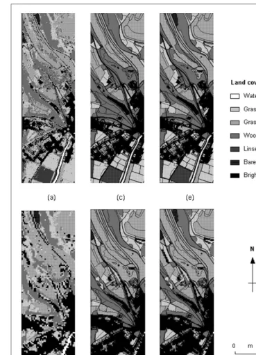
[image:3.675.319.569.45.306.2]Six stages of analysis were performed: (1) pre-processing, (2) per-pixel classification, (3) per-field classification, (4) missing
boundary flag, (5) per-field classification following the addi-tion of missing boundaries, and (6) accuracy assessment.
Pre-Processing
Prior to classification analysis, two pre-processing steps were implemented. First, theCASIimage and Land-Line data were co-registered to enable the integrated analysis required for subse-quent per-field classification. Because the Land-Line data were already registered to theBNG, theCASIimage was registered directly to the Land-Line data. Initially, 35 well distributed ground control points (GCPs) were identified on both data sets (CASIimage and Land-Line coverage). The two sets ofGCP coor-dinates were then compared to generate a second-order mathe-matical transform function. Finally, nearest-neighbor resam-pling was employed to transform theCASIimage to theBNGwith a root-mean-square error of 8.64 m.
Second, to enable a comparison between spatial resolu-tions of 4 m and 20 m, the original image was degraded to a spatial resolution of 20 m. A relatively simple method of image degradation was employed whereby the spectral values of the pixels in the original CASIimage were averaged to de-rive the spectral values of the pixels in the degraded image. This simple technique of image degradation has been prac-ticed widely (e.g., Heric et al., 1996), although it is acknowl-edged that some investigators have stressed the need to ac-count for additional factors, such as the signal-to-noise ratio (SNR) and the point spread function (PSF), in the process (e.g., Townshend and Justice, 1988). However, it was believed that the influence of these two factors on the degradation process was relatively minor and the omission of any measures to ac-count for them here did not affect the results significantly. For a fuller discussion on this point, see Aplin et al. (1999b). Per-Pixel Classification
Initially, seven land-cover classes were selected for classifica-tion (linseed, grassland 1, grassland 2, woodland, bare soil, water, and bright surfaces). The “grassland 1” class comprised relatively short, smooth grasses, while the “grassland 2” class comprised relatively long, rough grasses. A distinction be-tween these two classes may be explained more fully with re-spect to their landuse. The former class was largely agricul-tural and used for grazing livestock, while the latter was largely untended. A single “woodland” class was used for analysis be-cause wooded areas tended to be characterized by a mixture of deciduous species. Conifers were present in the study area but were relatively few and, where present, tended to combine with dominant deciduous species to form mixed forest stands. Several young woodland plantations were present, planted following severe storms in 1987 which devastated certain areas of woodland throughout the area. The “bright surfaces” class (a combination of asphalt, concrete, rooftiles, and so on) was used to represent urban areas.
Per-pixel classification was performed on the 4-m and 20-m spatial resolution images (Figures 2a and 2b, respectively). In each case, theMLclassifier was trained on a representative sam-ple of each of the classes, and a supervised classification was performed. In this study, classification was performed to com-pare per-pixel and per-field techniques rather than to appraise a specific per-pixel classification algorithm. Because it is a well-understood technique,MLclassification was an appropriate means of achieving this.
Per-Field Classification
To classify per field, the 4-m and 20-m spatial resolution per-pixel classified images were each combined with the Land-Line polygon coverage (Figures 2c and 2d, respectively). Initially, the raster CASIimage and vector Land-Line coverage were integrated using a GIS. To achieve this, the Land-Line data were rasterized such that each Land-Line polygon was represented by a pixel or a contiguous group of pixels. The
two raster data sets (CASIand Land-Line) were then combined in a single raster grid, enabling joint analysis.
To perform per-field classification, the modal land-cover class (the spatially dominant land-cover class) was assigned to each field (Land-Line polygon) in the combined raster grid. Specifically, the proportion of each field covered by each land-cover class was calculated. Then, for each field the class with the largest number of pixels (the modal land-cover class) was identified. Finally, this class value was reassigned to the entire field in the original vector (non-rasterized) Land-Line coverage.
Missing Boundary Flag
A major problem was encountered when attempting to clas-sify rural areas on a per-field basis. Numerous field bound-aries were missing, which resulted in the misclassification of entire fields. The absence of field boundaries led to the amal-gamation of multiple adjoining fields, regardless of any varia-tion in land cover, and resulted in the class of the spatially dominant field (that determining the modal land cover) being assigned incorrectly to the smaller fields. Incomplete or un-closed field boundaries (dangling vector lines) had the same result.
Initially, because the problem of missing field boundaries was associated primarily with large rural fields, a subset of the largest fields within the field site was selected for analysis. Fields with an area of greater than 8000 m2were selected. This
threshold was chosen so that the resulting subset provided an adequate and reasonable sample size and included all major rural fields. Fifty-three fields matched the criterion. Then, for each field, the proportion of modal land cover was extracted from the per-field classification, the local variance was calcu-lated, and the two values were compared.
Comparing Modal Land-Cover Proportion and Local Variance
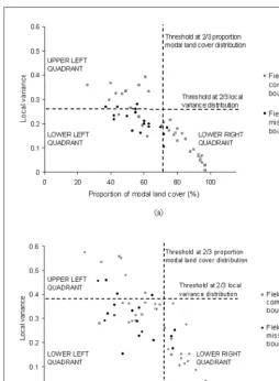
The proportion of modal land cover was plotted against the local variance on a per-field basis. This was performed for both 4-m and 20-m spatial resolution CASIimagery (Figures 3a and 3b, respectively). In general, the local variance of fields was considerably larger at the coarser (20-m) spatial resolu-tion. The mean local variance of the 53 fields at a spatial reso-lution of 20 m was greater than 0.28, while that of the same fields at a spatial resolution of 4 m was less than 0.20. This was largely a consequence of the direct relationship between (coarsening) spatial resolution and (decreasing) variance be-tween pixels (Woodcock and Strahler, 1987).
The values representing the proportion of modal land cover for each field were relatively similar between the 4-m and 20-m spatial resolution imagery. The mean proportion of modal land cover for the 53 fields at the finer spatial resolution was slightly less than 67 percent, approximately 3 percent greater than that of the same fields at the coarser spatial resolu-tion. Thus, although the scale of sampling changed, the pro-portions of land-cover classes remained relatively constant.
Automating the Procedure
Thresholds were selected to automate the procedure for se-lecting subsets of fields for manual checking. For each distrib-ution, thresholds were positioned at two thirds of the data range (Figures 3a and 3b), calculated as
thresholdmin(2(maxmin))3. (6)
The thresholds segmented the distribution of fields into quadrants, where the quadrants may be used to categorize the likely characteristics of the fields. The upper-left quadrants, where the local variance was large and the proportion of modal land cover was small, identified fields likely to be mixed. The lower-right quadrants, where the local variance was small and the proportion of modal land cover was large, identified fields likely to be homogeneous. For example, the
[image:5.675.125.495.49.560.2]cluster of fields in the lower-right quadrants of the distribu-tions in Figures 3a and 3b were predominantly large, homoge-neous agricultural fields. The lower-left quadrants, where both local variance and proportion of modal land cover were small, identified fields likely to have missing boundaries. For exam-ple, many of the fields at the lower left of the distributions in Figures 3a and 3b were large agricultural or semi-natural fields with missing boundaries. Fields within the latter quadrant Figure 2. Land-cover classifications based on the 4-m and 20-m spatial resolution
were subjected to manual checking. Within the 20-field subset selected using 4-m spatial resolution imagery, 14 fields with missing boundaries were identified. Within the 25-field subset selected using 20-m spatial resolution imagery, 11 fields with missing boundaries were identified.
Following manual checking, the vector data were edited manually to add missing field boundaries, thereby creating more accurate Land-Line polygon coverages (to be used in a second attempt at per-field classification). It should be noted that, for each spatial resolution, only those missing field boundaries identified previously using that spatial resolution were added for subsequent classification. That is, classifica-tion of the 4-m spatial resoluclassifica-tion imagery used vector data with the addition of missing boundaries for the 14 fields iden-tified using the missing boundary flag. Likewise, 11 fields were edited prior to subsequent classification of the 20-m spatial resolution imagery.
Accuracy of the Missing Boundary Flag
Prior to the continuation of classification analysis, it was deemed useful to assess the accuracy of the missing boundary flag at different spatial resolutions. (It is important to note that this is distinct from the assessment of “classification” accu-racy, which follows in the Accuracy Assessment section.) This involved, first, checking manually the entire population of 53 fields used in the missing boundary flag procedure to identify all missing boundaries. Eighteen fields had one or more miss-ing boundaries. This information was then cross-referenced with the plots comparing local variance and proportion of modal land cover (Figures 3a and 3b).
The missing boundary flag was considerably more accu-rate when using 4-m spatial resolution imagery than 20-m spatial resolution imagery (Table 1). A subset of 20 fields was selected using the former, of which 14 had missing bound-aries. Of the 33 fields excluded from selection, 29 had com-plete boundaries and were, therefore, omitted correctly. In contrast, a larger subset of 25 fields was selected using 20-m spatial resolution imagery. Not only did this subset require more processing time due to the larger number of fields, but only 11 fields with missing boundaries were included. Of those fields omitted, 21 out of 28 had complete boundaries and were omitted correctly. Overall, the missing boundary flag was over 20 percent more accurate when using the finer spa-tial resolution imagery. This can be illustrated with reference to the distributions of local variance and proportion of modal land cover. Fields with missing boundaries are most densely clustered in the lower-left quadrant of the plot at the finer spa-tial resolution (Figure 3a) than at the coarser spaspa-tial resolution (Figure 3b).
The main reason for the greater accuracy of this proce-dure at the finer spatial resolution was the greater detail pro-vided by this source of imagery. Considerable spatial autocor-relation was present in the 4-m spatial resolution imagery, enabling a relatively accurate delineation of homogeneous patches of land cover within fields. At the coarser spatial reso-lution, a considerably greater degree of mixing reduced the accuracy with which such homogeneous patches of land were identified.
Per-Field Classification Following the Addition of Missing Boundaries The per-pixel classified images were re-classified per field using the repaired Land-Line coverages (described in the Automating the Procedure section) for both the 4-m and 20-m spatial resolutionCASIimages (Figures 2e and 2f, respectively).
Accuracy Assessment
The accuracies of the six classifications (4 m per-pixel, 4 m per-field, and 4 m per-field following the addition of missing boundaries; 20 m per-pixel, 20 m per-field, and 20 m per-field following the addition of missing boundaries) were assessed by comparing the classified images to the reference land-cover map. The results are presented as kappa coefficients (Table 2). A per-pixel accuracy assessment procedure was carried out on both the per-pixel and per-field classifications; for this pur-pose, the latter were rasterized to the pixel size of the former. Then, random samples of pixels were selected for comparison with the reference land-cover map. It is acknowledged that
TABLE1. ACCURACY OF THEMISSINGBOUNDARYFLAG
Spatial Fields Included in Subset Fields Excluded from Subset Overall
Resolution Total Missing Accuracy Total Complete Accuracy Accuracy
of Image Number Boundaries (%) Number Boundaries (%) (%)
4 m 20 14 70 33 29 87.88 81.13
[image:6.675.31.285.48.394.2]20 m 25 11 44 28 21 75 60.38
[image:6.675.93.496.667.737.2]there are problems associated with assessing the accuracy of per-field classifications on a per-pixel basis. However, this pro-cedure had the benefits of weighting fields according to size (e.g., larger fields were more likely to be selected than smaller fields) and enabling a direct comparison between per-pixel and per-field classifications (Johnsson, 1994; Whiteet al., 1995). A full discussion of the implications of employing dif-ferent accuracy assessment procedures is provided in Aplin et al. (1999b).
Per-Pixel Versus Per-Field Classification
Generally, per-pixel classification was slightly less accurate than per-field classification (prior tothe addition of missing boundaries). For example, per-pixel classification of the 4-m spatial resolution CASIimage generated an overall kappa coefficient of 0.68, while per-field classification of the same image was marginally more accurate, with an overall kappa coefficient of 0.72. The main reason for this was spurious mis-classification at the per-pixel stage arising because of within-field spectral variation. Per-within-field classification, by aggregating to the modal land-cover class, removed such misclassification. However, although per-field classification was more accurate than per-pixel classification for most classes, certain classes were classified with a similar or lower accuracy by the per-field approach. One reason for this was that any increase in accuracy at the per-field stage arising through the removal of spurious within-field classification was offset by a decrease in accuracy caused by missing field boundaries. One extreme ex-ample of this was the bare soil class where per-pixel classifi-cation generated a kappa coefficient of 0.67 and per-field clas-sification generated a kappa coefficient of 0. The reason was that only a single field of bare soil was present in the study area and this field was missing from the Land-Line polygon coverage. Consequently, the field was amalgamated with a larger field of woodland and misclassified by the per-field classifier.
Missing Versus Complete Boundaries
While the original per-field classification of the 4-m spatial resolution CASIimage generated an overall kappa coefficient of 0.72, per-field classification following the addition of miss-ing boundaries generated an overall kappa coefficient of 0.84. While the accuracy of several classes remained relatively con-stant between these two, the accuracy of four predominantly rural classes (grassland 1, grassland 2, woodland, bare soil) increased considerably at the latter stage. The reason for this was the inclusion of formerly missing field boundaries in the
classification process. This prevented multiple fields from being amalgamated, thereby protecting subsidiary fields from misclassification. For instance, because the field of bare soil was present in the vector data, it was identified correctly. In fact, because this was the only major field of this class, all 50 sample points for bare soil were selected from it and the kappa coefficient was 1.
4-m Versus 20-m Spatial Resolution
Generally, classification using 4-m spatial resolution CASI im-agery was markedly more accurate than classification using 20-m spatial resolution imagery at each of the three stages of analysis (per-pixel, per-field, per-field following the addition of missing boundaries). This was primarily because consider-ably fewer mixed pixels were present in the finer spatial reso-lution imagery than in the coarser spatial resoreso-lution imagery. For instance, because the bright surfaces class comprised rela-tively small urban features, the 4-m spatial resolution data enabled more accurate identification of this class than did the 20-m spatial resolution data.
An additional factor affecting only the final stage of clas-sification (per-field following the addition of missing bound-aries) was that the missing boundary flag identified more fields with missing boundaries when using the 4-m spatial resolution imagery than when using the 20-m spatial resolu-tion imagery. This enabled a greater proporresolu-tion of missing field boundaries to be added prior to per-field classification of the 4-m spatial resolution imagery. Consequently, a greater degree of misclassification occurred in the 20-m spatial reso-lution imagery through the amalgamation of multiple fields where fields boundaries remained missing.
The most accurate classification overall was the per-field classification following the addition of missing boundaries using 4-m spatial resolution imagery. This generated an over-all kappa coefficient of 0.84. In comparison, the equivalent classification using 20-m spatial resolution imagery generated a kappa coefficient of 0.62.
Discussion
The national mapping agency of the United Kingdom, the Ordnance Survey, has recently converted their key spatial data product, Land-Line, into MasterMap™ as part of the Digital National Framework (DNF). This is a polygon data structure with associated topographical identifiers (TOIDs), and it will form a topographic base to which various attribute data layers will be attached. The role for remote sensing in producing national land-cover and land-use databases should be obvious, TABLE2. KAPPACOEFFICIENTS FORCLASSIFICATIONACCURACYASSESSMENT
Kappa Coefficients
4-m Spatial Resolution Image 20-m Spatial Resolution Image
Original Edited Original Edited
Land-Cover Per-Pixel Per-Field Per-Field Per-Pixel Per-Field Per-Field
Class Classification Classification Classification Classification Classification Classification
Linseed 0.75 0.93 0.89 0.79 0.88 0.88
Grassland 1 0.56 0.68 0.73 0.58 0.79 0.81
Grassland 2 0.62 0.63 0.79 0.59 0.36 0.65
Woodland 0.72 0.69 0.91 0.67 0.90 0.81
Bare soil 0.67 0 1 0.38 0 0.58
Water 0.82 0.79 0.75 0.28 0.06 0.05
Bright surfaces 0.64 0.74 0.81 0.59 0.67 0.65
Overall 0.68 0.72 0.84 0.55 0.55 0.62
presenting synergistic opportunities both to the Ordnance Survey and to the remote sensing communities.
The benefits of per-field classification over per-pixel classification have been demonstrated elsewhere (e.g., Aplin et al., 1999a). However, if per-field classification is to be accu-rate, then it will be necessary to check and potentially update the vector (or polygon) data on which it depends, prior to classification. This paper has demonstrated a simple method for detecting missing field boundaries based on a combination of the modal land cover and the average local variance per field. Three important discussion points follow.
First, “hard” per-pixel classification was used in this re-search. However, several studies have now demonstrated the benefits of soft classification over hard classification (e.g., Foody, 1999; Melgani et al., 2000; Cheng, 2002; Oki et al., 2002). There is no reason why soft classification should not be applied in the present context. The mode could be replaced by the maximum sum of soft land-cover proportions, and the local variance could be predicted using greater information content. An example of per-field classification using soft clas-sified imagery is provided by Aplin and Atkinson (2001).
Second, the mean local variance was predicted, which implies the decision to use a stationary model of local vari-ance. Such a decision means that potentially useful informa-tion is lost. For example, instead of predicting the mean, it may be possible to examine the entire cumulative distribution function (cdf) of values within each field or parcel. Interest-ingly, using the cdf does not make full use of the available data: the locations of each pixel, which are known, are ig-nored. One consequence is that it is not possible to say any-thing about wherewithin each parcel the missing boundaries ought to be located, only that a boundary might be missing. To locate potential boundaries, it is necessary to use an edge de-tection algorithm, or equivalent, per field. There are many to choose from including the Hough transform and the Sobel filter (Mather, 1999). It may even be possible to use the local variance (mapped within each field) for this purpose. A par-ticularly novel technique that may have application here is the so-called super-resolution mapping approach that takes a soft classification as input (described above) and maps land-cover boundaries within pixels (Tatem et al., 2001; Tatem et al., 2002). It is clear that the mean local variance represents only one relatively simple approach from the range of possi-bilities (e.g., Verhoeye and De Wulf, 2002).
Third, in this paper, arbitrary thresholds were used to predict missing boundaries from the proportion of modal land cover and the local variance. Many alternative approaches exist. For example, supervised classification could be used to potentially increase the accuracy of prediction. For example, for a large area containing many polygons, a small subset of polygons with (and without) missing boundaries could be used to train a supervised classifier. We chose to use un-trained thresholds because (1) they corresponded closely to the rationale given in the comparing Modal Land-Cover Pro-portion and Local Variance section for use of the proPro-portion of modal land cover and local variance (that is, they illustrate the concept well), and (2) such a procedure might be useful where training is not viable (e.g., very large areas of interest). In any case, the purpose of this paper was to explore and il-lustrate the potential use of the two variables, not to design the technique used to extract information from them.
Conclusions
Five specific conclusions can be made:
•
per-pixel classification of land cover resulted in misclassifica-tion due to within-field variamisclassifica-tion;•
per-field classification removed this source of misclassifica-tion but missing field boundaries led to entire fields being misclassified;•
missing boundaries were predicted by comparing within-field modal land-cover proportion and local variance, increasing per-field classification accuracy subsequently;•
4-m spatial resolution imagery was considerably more accu-rate than 20-m spatial resolution imagery for predicting miss-ing boundaries fields; and, therefore,•
4-m spatial resolution imagery was considerably more accu-rate than 20-m spatial resolution imagery for classifying land cover in rural areas.References
Aplin, P., P.M. Atkinson, and P.J. Curran, 1997. Fine spatial resolution satellite sensors for the next decade, International Journal of Re-mote Sensing, 18:3873–3881.
, 1998. Identifying missing field boundaries to increase the ac-curacy of per-field classification of fine spatial resolution satellite sensor imagery, Proceedings of the 27th International Symposium on Remote Sensing of Environment: Information for Sustainabil-ity, 08–12 June, Tromso, Norway, Norwegian Space Centre, Oslo, Norway, pp. 399–402.
, 1999a. Fine spatial resolution simulated satellite sensor im-agery for land cover mapping in the UK, Remote Sensing of Envi-ronment, 68:206–216.
, 1999b. Per-field classification of land use using the forthcom-ing very fine spatial resolution satellite sensors: problems and po-tential solutions, Advances in Remote Sensing and GIS Analysis (P. Atkinson and N. Tate, editors), John Wiley, Chichester, United Kingdom, pp. 219–239.
Aplin, P., and P.M. Atkinson, 2001. Sub-pixel land cover mapping for per-field classification, International Journal of Remote Sensing, 22:2853–2858.
Berberoglu, S., and P.J. Curran, 2000. Utilising texture measures in an artificial neural network for the per-field classification of agricul-tural land cover in the Mediterranean,Aspects of Applied Biology, 60:21–28.
Chan, J.C.-W., K.-P. Chan, and A.G.-O. Yeh, 2001. Detecting the nature of change in an urban environment: A comparison of machine learning algorithms, Photogrammetric Engineering & Remote Sensing, 67:213–225.
Cheng, T., 2002. Fuzzy objects: their changes and uncertainties, Pho-togrammetric Engineering & Remote Sensing, 68:41–49. Congalton, R.G., 1991. A review of assessing the accuracy of
classifi-cations of remotely sensed data, Remote Sensing of Environment, 37:35–46.
Cortijo, F.J., and N.P. De La Blanca, 1998. Improving classical contex-tual classifications, International Journal of Remote Sensing, 19:1591–1613.
Cushnie, J.L., 1987. The interactive effect of spatial resolution and degree of internal variability within land-cover types on classifi-cation accuracies, International Journal of Remote Sensing, 8:15–29.
Foody, G.M., 1996. Approaches for the production and evaluation of fuzzy land cover classifications from remotely-sensed data, Inter-national Journal of Remote Sensing, 17:1317–1340.
, 1999. The continuation of classification fuzziness in thematic mapping, Photogrammetric Engineering & Remote Sensing, 65: 443–451.
Foody, G.M., N.A. Campbell, N.M. Trodd, and T.F. Wood, 1992. De-rivation and applications of probabilistic measures of class mem-bership from the maximum-likelihood classification, Photogram-metric Engineering & Remote Sensing, 58:1335–1341.
Frizzelle, B.G., and A. Moody, 2001. Mapping continuous distribu-tions of land cover: A comparison of maximum-likelihood esti-mation and artificial neural networks, Photogrammetric Engineer-ing & Remote SensEngineer-ing, 67:693–705.
Fuller, R.M., G.B. Groom, and A.R. Jones, 1994. The land cover map of Great Britain: An automated classification of Landsat Thematic Mapper data, Photogrammetric Engineering & Remote Sensing, 60:553–562.
commercial satellite imagery, Photogrammetric Engineering & Re-mote Sensing, 62:279–284.
Irons, J.R., B.L. Markham, R.F. Nelson, D.L. Toll, D.L. Williams, R.S. Latty, and M.L. Stauffer, 1985. The effects of spatial resolution on the classification of Thematic Mapper data, International Journal of Remote Sensing, 6:1385–1403.
Janssen, L.L.F., M.N. Jaarsma, and T.M. Van der Linden, 1990. Inte-grating topographic data with remote sensing for land-cover clas-sification, Photogrammetric Engineering & Remote Sensing, 56: 1503–1506.
Janssen, L.L.F., and F.J.M. van der Wel, 1994. Accuracy assessment of satellite derived land-cover data: A review, Photogrammetric En-gineering & Remote Sensing, 60:419–426.
Janssen, L.L.F., and M. Molenaar, 1995. Terrain objects, their dynamics and their monitoring by the integration of GIS and remote sensing, IEEE Transactions on Geoscience and Remote Sensing, 33:749–758. Ji, C.Y., 2000. Land-use classification of remotely sensed data using
Kohonen self-organizing feature map neural networks, Pho-togrammetric Engineering & Remote Sensing, 66:1451–1460. Johnsson, K., 1994. Segment-based land-use classification from SPOT
satellite data, Photogrammetric Engineering & Remote Sensing, 60:47–53.
Mason, D.C., D.G. Corr, A. Cross, D.C. Hogg, D.H. Lawrence, M. Petrou, and A.M. Tailor, 1988. The use of digital map data in the segmen-tation and classification of remotely-sensed images,International Journal of Geographical Information Systems, 9:195–215. Mather, P.M., 1999. Computer Processing of Remotely-Sensed Images:
An Introduction,Second Edition, John Wiley, Chichester, United Kingdom, 292 p.
Mattikalli, N.M., B.J. Devereux, and K.S. Richards, 1995. Integration of remotely sensed satellite images with a geographical informa-tion system, Computers and Geosciences, 21:947–956.
Melgani, F., B.A. Al Hashemy, and S.M. Taha, 2000. An explicit fuzzy supervised classification method for multispectral remote sensing images, IEEE Transactions on Geoscience and Remote Sensing, 38:287–295.
Nishii, R., and S. Tanaka, 1999. Accuracy and inaccuracy assessments in land-cover classification, IEEE Transactions on Geoscience and Remote Sensing, 37:491–498.
Oki, K., H. Oguma, and M. Sugita, 2002. Subpixel classification of alder trees using multitemporal Landsat Thematic Mapper im-agery, Photogrammetric Engineering & Remote Sensing, 68:77–82. Ortiz, M.J., A.R. Formaggio, and J.C.N. Epiphanio, 1997. Classification of croplands through integration of remote sensing, GIS and his-torical database, International Journal of Remote Sensing, 18: 95–105.
Palacio-Prieto, J.L., and L. Luna-González, 1996. Improving spectral results in a GIS context, International Journal of Remote Sensing, 17:2201–2209.
San Miguel-Ayanz, J., and G.S. Biging, 1997. Comparison of single-stage and multi-single-stage classification approaches for cover type mapping with TM and SPOT data, Remote Sensing of Environ-ment, 59:92–104.
Settle, J.J., and S.A. Briggs, 1987. Fast maximum likelihood classifica-tion of remotely-sensed imagery, Internaclassifica-tional Journal of Remote Sensing, 8:723–734.
Smith, G., R. Fuller, G. Amable, C. Costa, and B. Devereux, 1997. CLassification of Environment with VEctor-and Raster Mapping (CLEVER mapping), Proceedings of GISRUK97, 09–11 April, University of Leeds, Leeds, United Kingdom, pp. 70–72.
Smith, G.M., R.M. Fuller, and B.J. Devereux, 1998. An integrated vector/raster system for land cover mapping, IEE Coloquium Digest—Integrated Systems for Commercial Remote Sensing Applications, Institute of Electrical Engineers, London, United Kingdom, pp. 2/1–2/6.
Smith, J.H., J.D. Wickham, S.V. Stehman, and L. Yang, 2002. Impacts of patch size and land-cover heterogeneity on thematic image classification accuracy, Photogrammetric Engineering & Remote Sensing, 68:65–70.
Stehman, S.V., 1997. Selecting and interpreting measures of thematic classification accuracy, Remote Sensing of Environment, 62: 77–89.
Tatem, A.J., H.G. Lewis, P.M. Atkinson, and M.S. Nixon, 2001. Land cover mapping from remotely sensed images at the sub-pixel scale using a Hopfield neural network, IEEE Transactions on Geoscience and Remote Sensing, 39:781–796.
, 2002. Super-resolution land cover pattern prediction using a Hopfield Neural Network, Remote Sensing of Environment, 79: 1–14.
Thomas, I.L., V.M. Benning, and N.P. Ching, 1987. Classification of Remotely Sensed Images, Adam Hilger, Bristol, United Kingdom, 256 p.
Townshend, J.R.G., 1992. Land cover, International Journal of Remote Sensing, 13:1319–1328.
Townshend, J.R.G., and C.O. Justice, 1988. Selecting the spatial reso-lution of satellite sensors required for global monitoring of land transformations, International Journal of Remote Sensing, 9:187–236.
Tsang, T., and M. Barnsley, 1996. A comparative analysis of various methods for quantifying landscape heterogeneity, Proceedings of RSS’96: Remote Sensing Science and Industry, 11–14 September, University of Durham, Durham, United Kingdom (Remote Sens-ing Society, NottSens-ingham, United KSens-ingdom), pp. 513–520. Tso, B.C.K., and P.M. Mather, 2001. Classification Methods for
Re-motely Sensed Data, Taylor and Francis, New York, N.Y., 332 p. Verhoeye, K.J., and R. De Wulf, 2002. Land cover mapping at
sub-pixel scales using linear optimization techniques, Remote Sens-ing of Environment, 79:96–104.
Wang, R.S.M., S.A. Roberts, and N.D. Efford, 1997. An object-based approach to integrate Landsat TM data within a GIS context for detecting land use changes at urban-rural fringe areas, Proceed-ings of RSS’97: Observations and Interactions, 02–04 September, University of Reading, Reading, United Kingdom (Remote Sens-ing Society, NottSens-ingham, United KSens-ingdom), pp. 179–184. Westmoreland, S., and D.A. Stow, 1992. Category identification of
changed land-use polygons in an integrated image processing/ geographic information system, Photogrammetric Engineering & Remote Sensing, 58:1593–1599.
White, J.D., G.C. Kroh, and J.E. Pinder III, 1995. Forest mapping at Lassen Volcanic National Park, California, using Landsat TM data and a geographical information system, Photogrammetric Engi-neering & Remote Sensing, 61:299–305.
Woodcock, C.E., and A.H. Strahler, 1987. The factor of scale in remote sensing, Remote Sensing of Environment, 21:311–332.
Yang, H., F. van der Meer, W. Bakker, and Z.J. Tan, 1999. A back-propagation neural network for mineralogical mapping from AVIRIS data, International Journal of Remote Sensing, 20:97–110.