PDE–CONSTRAINED OPTIMIZATION PROBLEM INVOLVING
THE GENERALIZED OSEEN EQUATIONS.∗
ALEJANDRO ALLENDES†, ENRIQUE OT ´AROLA‡, AND RICHARD RANKIN§
Abstract. We derive globally reliable a posteriori error estimators for a linear–quadratic optimal control problem involving the generalized Oseen equations as state equations; control constraints are also considered. The corresponding local error indicators are locally efficient. The assumptions under which we perform the analysis are such that they can be satisfied for a wide variety of stabilized finite element methods as well as for standard finite element methods. When stabilized methods are considered, no a priori relation between the stabilization terms for the state and adjoint equations is required. If a lower bound for the inf–sup constant is available, a posteriori error estimators that are fully computable and provide guaranteed upper bounds on the norm of the error can be obtained. We illustrate the theory with numerical examples.
Key words. linear–quadratic optimal control problems; generalized Oseen equations; Brinkman equations; Stokes equations; a posteriori error estimators; stabilized adaptive finite element methods.
AMS subject classifications.49K20, 49M25, 65K10, 65N15, 65N30, 65N50, 65Y20.
1. Introduction. In this work we shall be interested in the design and analy-sis of computable a posteriori error estimators for a linear–quadratic optimal control problem involving the generalized Oseen equations; control constraints are also con-sidered. To make matters precise, let Ω ⊂ Rd, with d ∈ {2,3}, be an open and bounded polytopal domain with Lipschitz boundary ∂Ω and f ∈ L2(Ω)d. Given a regularization parameterϑ >0 and a desired stateyΩ∈L2(Ω)d, we define
(1.1) J(y,u) =1
2ky−yΩk
2
L2(Ω)d+ ϑ
2kuk
2
L2(Ω)d.
We will be interested in the following PDE–constrained optimization problem: Find
(1.2) minJ(y,u)
subject to thegeneralized Oseen equations
(1.3)
−ε∆y+ (c· ∇)y+κy+∇p = f+u in Ω,
∇ ·y = 0 in Ω,
y = 0 on∂Ω,
and the control constraints
(1.4) a≤u≤b a.e. in Ω,
with a,b ∈ Rd satisfying a < b; the previous vector inequalities being understood componentwise. In (1.3),ε, κ∈Rand are such thatε >0 andκ≥0 andc∈W1,∞(Ω)
∗Funding: Alejandro Allendes was supported by CONICYT through FONDECYT project
1170579. Enrique Ot´arola was supported by CONICYT through FONDECYT project 3160201. Richard Rankin was partially supported by BASAL PFB03 CMM project, Universidad de Chile.
†Departamento de Matem´atica, Universidad T´ecnica Federico Santa Mar´ıa, Valpara´ıso, Chile
‡Departamento de Matem´atica, Universidad T´ecnica Federico Santa Mar´ıa, Valpara´ıso, Chile
§School of Mathematical Sciences, University of Nottingham Ningbo China, Ningbo, China
is a solenoidal field. The generalized Oseen equations describe the low–Reynolds– number flow in porous media in situations where velocity gradients are non–negligible; they provide a unified approach to model flows of viscous fluids in a cavity and a porous media. It is well–known that the following choices of the parameters c and κyield the following flow models:
(1.5)
c=0, κ= 0 :−ε∆y+∇p (Stokes),
c=0 :−ε∆y+κy+∇p (Brinkman), κ= 0 :−ε∆y+ (c· ∇)y+∇p (Oseen).
Our analysis allows for these choices of c andκ. Consequently, we present a unified analysis for the Stokes, Brinkman, Oseen and generalized Oseen equations.
The design of numerical techniques for approximating the solution to (1.3) has two major difficulties: first, in view of the so–called inf–sup condition [23, 24], arbi-trary finite element methods are not allowed, and second, considering standard finite element methods produces poor approximation results when convection–dominated regimes are considered [38]. In order to overcome such difficulties, a variety of finite element techniques have been proposed and analyzed in the literature: the family of stabilized finite element methods. We refer the reader to [38] for an extensive overview. In the PDE–constrained optimization context, a usual alternative for approximat-ing the solution to the optimal control problem (1.2)–(1.4) is based on the so-called optimize–then–discretize approach. This technique discretizes the associated optimal-ity system: the state equations (1.3), the adjoint equations and a variational inequaloptimal-ity that characterizes the optimal control ¯u. Consequently, the difficulties presented in the discretization of (1.3) are also present in the numerical approximation of the so-lution to (1.2)–(1.4). In addition, (1.2)–(1.4) is intrinsically nonlinear and, if c6=0, presents a crosswind phenomena; the convection field of the adjoint equations is the negative of the one appearing in (1.3). The latter further motives the development of an efficient solution technique that, in convection–dominated regimes, properly treats the oscillatory behaviors that occur when approximating ¯y and its adjoint variable
¯
w and resolves interior or boundary layers exhibited by both variables. Failure to resolve boundary layers can pollute the numerical solution in the entire domain; see [25] for results involving the scalar version of (1.2)–(1.4). However, numerical schemes based only on stabilized techniques are not sufficient to approximate the solution to (1.2)–(1.4): in addition to the efficient resolution of either interior or boundary layers, some possible geometric singularities must be resolved. This motivates the methods that we will use in this work: stabilized adaptive finite element methods.
In the current work, the assumptions under which we perform the analysis are such that they can be satisfied for a wide variety of stabilized finite element methods as well as for standard finite element methods. This includes using a different stabilization method to approximate the state equation from that used to approximate the adjoint equation. We derive a posteriori error estimators that are globally reliable. Moreover, if a lower bound for the inf–sup constant is available, we can obtain a posteriori error estimators that are fully computable and provide guaranteed upper bounds on the norm of the error. Consequently, the estimators can be used as a stopping criterion in adaptive algorithms. The local error indicators that can be used to adaptively refine the mesh are locally efficient. Furthermore, we observe that they can be used to efficiently resolve boundary layers.
The outline of this paper is as follows. In section2we introduce some terminology used throughout this work. In section3we study the optimal control problem (1.2)– (1.4) and obtain the associated optimality system. In section 4 we give the general form of the finite element methods that we consider for approximating the solution to (1.2)–(1.4). The core of our work is section5, where we devise a family of a posteriori error estimators. Under suitable assumptions, we obtain abstract reliability results in section5.1and local efficiency of the corresponding error indicators in section5.2. In section6we consider the estimators that we can obtain for a particular approximation method in more detail. Finally, in section7we present a series of numerical examples to illustrate the theory.
2. Preliminaries.
2.1. Notation. For a bounded domainA⊂Rt,t∈ {1,2,3},L2(A) andH1(A)
denote the standard Lebesgue and Sobolev spaces, respectively;L2
0(A) is the subspace
ofL2(A) containing functions with zero mean value onA, andH1
0(A) is the subspace
of H1(A) containing functions whose trace is zero on ∂A. We use bold letters to
denote the vector–valued counterparts of the aforementioned spaces and an extra under accent for their matrix–valued counterparts. For instance, ford ∈ {2,3}, we denoteL2(A) =L2(A)d andL
≈
2(A) =L2(A)d×d.
We now proceed to define notation associated with the discretization of the do-main. Let T = {K} be a conforming partition of ¯Ω into simplicial elements K [18,23]. We assume thatT is a member of a shape regular family of partitions. Let F denote the set of all element edges(2D)/faces(3D) and FI ⊂ F denote the set of interior edges(2D)/faces(3D).
For an elementK∈T, let:
• Pn(K) denote the space of polynomials onK of total degree at mostn; • FK⊂ F denote the set containing the individual edges(2D)/faces(3D) ofK; • hK denote the diameter ofK;
• nKγ denote the unit exterior normal vector to the edge(2D)/face(3D)γ∈ FK. For an edge(2D)/face(3D)γ∈ F, let:
• Pn(γ) denote the space of polynomials onγ of total degree at mostn; • Ωγ ={K∈T : γ∈ FK};
• hγ denote the diameter of the edge(2D)/face(3D)γ.
To simplify the exposition of the material, we defineV=H10(Ω) andQ=L20(Ω)
with norms||| · |||V,Ωand||| · |||Q,Ωdefined, for allξ∈V andφ∈Q, by
(2.1) |||ξ|||2V,Ω:=
X
K∈T
|||ξ|||2V,K and|||φ|||
2
Q,Ω:=
X
K∈T
where
(2.2) |||ξ|||2V,K :=εk∇ξk
2 L ≈
2(K)+κkξk2L2(K)and|||φ||| 2
Q,K :=kφk
2
L2(K).
The relation a . b indicates that there exists a constant C such that a ≤Cb. The constant C may be different at each occurrence but is independent ofa, b and the size of the elements in the mesh.
2.2. Inequalities. ForK ∈T and nonnegative integers l, we denote by ΠK,l theL2(K)–orthogonal projection operator ontoPl(K)d. This operator is defined as (2.3) ΠK,l:L2(K)→Pl(K)d, (t
−ΠK,l(t),v)L2(K)= 0 ∀v∈Pl(K)d.
Throughout the manuscript we will frequently make use of the following inequal-ities. First, ifK∈T andξ∈V, we have the Poincar´e inequalities [10,33,37] (2.4) kξkL2(Ω)≤CP,Ωk∇ξkL
≈
2(Ω)and kξ−ΠK,0(ξ)kL2(K)≤hK π k∇ξkL≈
2(K),
where
(2.5) CP,Ω= 1
π
d X
i=1
1 |li|2
!−1/2
with|l1|, . . . ,|ld|being the sides of ad-dimensional box containing Ω. We immediately comment that these inequalities imply that, forξ∈VandK∈T,
(2.6) kξkL2(Ω)≤CΩ|||ξ|||V,Ωand kξ−ΠK,0(ξ)kL2(K)≤CK|||ξ|||V,K,
where
(2.7) CΩ=
( CP,Ω
√ε, ifκ= 0,
minnC√P,Ω
ε,
1
√κ o
, ifκ6= 0,
and
(2.8) CK=
( hK
π√ε, ifκ= 0, minnhK
π√ε,
1
√κ o
, ifκ6= 0.
We defineA:V×V→R,B:V×Q→RandC:V×V→Rby
(2.9)
A(ξ,ζ) :=ε(∇ξ,∇ζ)L≈2(Ω)+ (κξ+ (c· ∇)ξ,ζ)L2(Ω),
B(ζ, φ) := (φ,∇ ·ζ)L2(Ω),
C(ξ,ζ) :=ε(∇ξ,∇ζ)L≈2(Ω)+ (κξ−(c· ∇)ξ,ζ)L2(Ω).
The fact thatcis a solenoidal vector field and integration by parts implies that
(2.10) A(ξ,ζ) =C(ζ,ξ) ∀ξ,ζ∈V.
Moreover, for allξ∈V,
and, for allξ,ζ∈V,
(2.12) A(ξ,ζ)≤Cct|||ξ|||
V,Ω|||ζ|||V,Ω, C(ξ,ζ)≤Cct|||ξ|||V,Ω|||ζ|||V,Ω,
where
(2.13) Cct= 1 +
CΩ
√εk|c|kL∞(Ω),
withk|c|kL∞(Ω)being theL∞(Ω) norm of|c|andCΩbeing given by (2.7).
We now recall the standard inf–sup condition [23, 24]: there exists a positive constantβ such that
(2.14) βkφkL2(Ω)≤ sup ξ∈V\{0}
B(ξ, φ) k∇ξkL≈2(Ω) ∀
φ∈Q.
Notice that, in view of|||ξ|||2V,Ω≤(ε+κC2P,Ω)k∇ξk2L≈2(Ω), we have that
(2.15) |||φ|||Q,Ω≤Cis sup
ξ∈V\{0}
B(ξ, φ) |||ξ|||V,Ω
∀φ∈Q,
where
(2.16) Cis=
q
ε+κC2
P,Ω
β .
3. Optimal control problem: optimize. In this section we briefly analyze the optimal control problem (1.2)–(1.4). To accomplish this task, we begin by introducing the following weak version of the state equations (1.3): Find (y,p)∈V×Qsuch that (3.1)
A(y,ξ)− B(ξ,p) = (f+u,ξ)L2(Ω) ∀ξ∈V,
B(y, φ) = 0 ∀φ∈Q,
where the bilinear formsAandBare defined by (2.9) and we recall thatε >0,κ≥0,
c∈W1,∞(Ω) is a solenoidal field,f ∈L2(Ω),V=H10(Ω) andQ=L20(Ω). In view of
the fact thatAsatisfies (2.11) and (2.12) andBsatisfies the inf–sup conditions (2.14) and (2.15), we conclude the well–posedness of problem (3.1) [23,24]. We also mention that, due to de Rham’s Theorem (see Section 4.1.3 and Theorem B73 in [23]), we can consider the following equivalent formulation of problem (3.1): Findy∈V0such that
(3.2) A(y,ξ) = (f+u,ξ)L2(Ω) ∀ξ∈V0,
whereV0:={v∈H10(Ω) : ∇ ·v= 0}.
To analyze our optimal control problem, we follow [30,44] and introduce the so– called control to state mapS:L2(Ω)→V0 which, given a controlu, associates to it
the statey that solves (3.2). In addition, we define, fora,b∈Rd witha<b, the set (3.3) Uad:={v∈L2(Ω) : a≤v≤b a.e. in Ω};
the vector inequalities being understood componentwise. The setUadis a bounded, convex, closed and nonempty subset of L2(Ω) and consequently weakly sequentially compact. Thus, in view of the fact that the reduced cost functional
f(u) := 1
2kS(u)−yΩk
2 L2(Ω)+
ϑ
2kuk
is weakly lower semicontinuous and strictly convex (ϑ >0), we conclude the existence and uniqueness of an optimal control ¯u and an optimal state ¯y that satisfy (3.2), or equivalently (3.1); see Theorem 2.14 in [44]. The existence of ¯p such that (¯y,¯p) solves (3.1) follows from de Rham’s Theorem. In addition, we have that ¯u satisfies the first–order optimality condition
(3.4) f′(¯u)(u−u¯)≥0 ∀ u∈Uad;
see [44, Lemma 2.21]. To explore this variational inequality, and to obtain optimality conditions, we define, on the basis of the formal Lagrange method (see [21, Section 3.3] and [44, Section 2.10]), the adjoint state (w,q) as the unique solution to the following weak problem: Find (w,q)∈V×Qsuch that
(3.5)
C(w,ζ) +B(ζ,q) = (y−yΩ,ζ)L2(Ω) ∀ζ∈V,
B(w, ψ) = 0 ∀ψ∈Q.
With this adjoint state at hand, the variational inequality (3.4) can be rewritten as
(3.6) ( ¯w+ϑ¯u,u−u¯)L2(Ω)≥0 ∀ u∈Uad.
We have thus arrived at the following optimality system: (¯y,¯p,u¯) ∈ V×Q×Uad is optimal for the PDE–constrained optimization problem (1.2)–(1.4) if and only if (¯y,¯p,w¯,¯q,u¯)∈V×Q×V×Q×Uadsolves
(3.7)
A(¯y,ξ)− B(ξ,¯p) = (f+ ¯u,ξ)L2(Ω), ∀ξ∈V,
B(¯y, φ) = 0, ∀φ∈Q,
C( ¯w,ζ) +B(ζ,¯q) = (¯y−yΩ,ζ)L2(Ω), ∀ζ∈V,
B( ¯w, ψ) = 0, ∀ψ∈Q,
( ¯w+ϑu¯,u−¯u)L2(Ω) ≥ 0, ∀u∈Uad;
see also [39, Section 2] and [34, Section 2] for similar results when the state equations (1.3) are the Stokes equations.
We finally recall the projection formula for the optimal control variable: the variational inequality in (3.6) can be equivalently written as [44, Chapter 2]
(3.8) u¯= Π[a,b]
−ϑ1w¯
a.e. in Ω,
where Π[a,b](ζ) (x) := min{b,max{a,ζ(x)}} and it is understood componentwise.
We note that
(3.9)
Π[a,b](ξ)−Π[a,b](ζ)
L2(K)≤ kξ−ζkL2(K) ∀ξ,ζ∈V.
4. Finite element discretization. We follow theoptimize–then–discretize ap-proach and introduce a numerical scheme to approximate the solution to (3.7). The scheme allows for the incorporation of stabilization terms into the standard Galerkin discretizations of the state and adjoint equations; no a priori relation between the stabilized terms is required. We refer the reader to Remark4.1below for a discussion regarding the advantages of the proposed approach when solving (1.2)–(1.4).
The stabilized scheme reads as follows: Find (¯yT,¯pT,w¯T,q¯T,¯uT) ∈ V(T)×
Q(T)×V(T)×Q(T)×Uad(T) such that
(4.1)
A(¯yT,ξ)− B(ξ,¯pT) +S(¯yT,p¯T,f+ ¯uT;ξ) = (f+ ¯uT,ξ)L2(Ω),
B(¯yT, φ) +H(¯yT,p¯T,f+ ¯uT;φ) = 0,
C( ¯wT,ζ) +B(ζ,¯qT) +Q( ¯wT,¯qT,¯yT −yΩ;ζ) = (¯yT −yΩ,ζ)L2(Ω),
B( ¯wT, ψ) +K( ¯wT,¯qT,¯yT −yΩ;ψ) = 0,
for all (ξ, φ,ζ, ψ,u)∈V(T)×Q(T)×V(T)×Q(T)×Uad(T); the bilinear forms A,BandCbeing defined as in (2.9). We consider the setting where the discrete spaces
V(T) andQ(T) are subspaces ofVandQ, respectively, and the discrete setUad(T) is a subset ofUad. Hence,V(T)⊂V, Q(T)⊂Qand Uad(T)⊂Uad. The terms S andH, andQ and K in (4.1), correspond to stabilization terms for the state and adjoint equations, respectively. Finally, we assume thatV(T), Q(T), Uad(T), S, H,QandK are such that at least one solution to (4.1) exists.
Remark 4.1 (optimize–then–discretize approach). In general, there are two ap-proaches to approximate the solution to an optimal control problem: the optimize– then–discretize approach, that discretizes the associated optimality system, and the discretize–then–optimize approach, that first discretizes the continuous problem and then optimizes the obtained finite dimensional problem. We must immediately com-ment that these techniques do not always coincide [16, 19, 26, 29]. For a detailed discussion on these approaches and their respective advantages and disadvantages, we refer the reader to [26, Section 3.2] and [15, Chapter 3]. In [19], it was observed that, when solving an optimal control problem for a convection–reaction–difussion equation on the basis of the SUPG method, both approaches lead to substantially dif-ferent results. Later, in [25], the authors continue with the study started in [19] and show that the failure to resolve boundary layers exhibited by the solution can pollute the numerical solution in the entire domain. In order to develop our a posteriori error analysis, we follow theoptimize–then–discretize approach. This allows for the simple formulation (4.1) of the discrete optimality system and the incorporation of stabi-lization terms into the discrete state and adjoint equations; no a priori relationship between such stabilization terms is required. We remark that the latter property is particularly convenient since it allows for the use of the a posteriori error estimators that are already available in the literature. In contrast, the use of thediscretize–then– optimize approach imposes a relationship between the stabilization terms which could result in the presence of undesirable stabilization terms in the discrete formulation. If both termsS andHare symmetric andQ=S andK=H, then the aforementioned approaches coincide; we refer the reader to [16] for details.
Before proceeding with the analysis of our method, it is instructive to comment on those advocated in the literature. Regarding the a priori theory, in the absence of control constraints, the design and analysis of numerical techniques for solving (1.2)– (1.3), withc=0andκ= 0, have been investigated in several papers; see [14,40,42] and references therein. To the best of our knowledge, and again, forc=0andκ= 0, the first work that incorporates control constraints and analyzes stabilized schemes for (1.2)–(1.4) is [39]; the optimal control is discretized by using piecewise constant functions. The authors, on the basis of postprocessing techniques, provide a quadratic error estimate for the approximation of the optimal control variable [39, Theorem 2.8]. Subsequently, the authors of [34] extend the results of [39] and analyze nonconforming schemes for the discretization of the state and adjoint equations; in contrast to [39], the vector field is not assumed to be inH2(Ω)∩W1,∞(Ω). In addition, [34] analyzes an anisotropic scheme for approximating the solution to (1.2)–(1.4) when Ω is not convex; a domain with a reentrant edge (d = 3) is considered. We conclude this paragraph by mentioning the reference [22], where the authors investigate numerical techniques for solving a modification of problem (1.2)–(1.4) that, in addition, includes constraints on the state variable.
work, the authors follow the discretize–then–optimize approach and obtain a discrete optimality system with no stabilization terms [32, equation (2.9)]. They propose an error estimator in a two–dimensional setting and analyze its reliability properties [32, Theorem 3.1]. However, there is no efficiency analysis. Later, an asymptotically exact ZZ–type a posteriori error estimator was proposed in [31]. The authors derive upper and lower bounds for the error in terms of the proposed estimator [31, Theorem 5.1] that relies on an error non–degeneracy condition [31, inequality (2.24)] and strong regularity assumptions on (¯y,¯p): it is assumed to belong toH3(Ω)∩V×H1(Ω)∩Q
[31, Lemma 4.2]. In [20], the authors propose an a posteriori error estimator for (1.2)– (1.4) but with the state equations (1.3) replaced by a Stokes-Darcy system: they study the reliability and efficiency properties of the proposed estimator. We also mention [35], where a similar PDE–constrained optimization problem has been analyzed but with the control constraint (1.4) replaced by the state constraintkykL2(Ω)≤γ, where γ >0: an error estimator is proposed and its reliability and efficiency properties are investigated. All the aforementioned references consider plain Galerkin discretizations for the state and adjoint equations, i.e., no stabilization terms are considered. We conclude this paragraph by mentioning the so–called dual weighted residual method (DWR) [13] and its applications to the optimal control of flow problems [11,12].
Recently, the authors of [28] propose and analyze an a posteriori error estimator for problem (1.2)–(1.4) when κ = 0 [28, Section 5]. The associated discrete opti-mal system incorporates stabilized terms, into the state and adjoint equations, that are based on the streamline–diffusion finite element method (SDFEM). On the ba-sis of proposed and analyzed a posteriori error estimators for the state and adjoint equations, the authors derive an estimator for (1.2)–(1.4). We comment that the ob-tained upper bound for the error, in terms of the a posteriori error estimator, is not computable.
In this work we analyze a family of a posteriori error estimators in a unifying framework that incorporates a wide variety of standard and stabilized finite element methods.
5. A posteriori error analysis. In this section we derive and analyze a poste-riori error estimators for the solution to the discretization (4.1) of the optimal control problem (3.7).
5.1. Reliability analysis. We begin this section by introducing the following notation. Letey:= ¯y−¯yT,ep:= ¯p−¯pT,ew:= ¯w−w¯T,eq:= ¯q−¯qT andeu:= ¯u−u¯T,
where (¯y,¯p,w¯,¯q,u¯)∈V×Q×V×Q×Uad is the solution to the optimality system (3.7) and (¯yT,¯pT,w¯T,¯qT,u¯T)∈V(T)×Q(T)×V(T)×Q(T)×Uad(T) is its
numerical approximation given as the solution to (4.1). The goal of this section is to obtain an upper bound for
(5.1) |||(ey,ep,ew,eq,eu)|||2Ω:=
X
K∈T
|||(ey,ep,ew,eq,eu)|||2K
where
|||(ey,ep,ew,eq,eu)|||2K :=|||ey|||2V,K+̺|||ep|||
2
Q,K+|||ew|||
2
V,K+̺|||eq|||2Q,K+keuk2L2(K).
The upper bound for the error (5.1) that we obtain is constructed using upper bounds on the error between the solution to the discretization (4.1) and auxiliary variables that we define in what follows. Let (ˆy,ˆp)∈V×Qbe the solution to (5.2)
A(ˆy,ξ)− B(ξ,ˆp) = (f+ ¯uT,ξ)L2(Ω) ∀ξ∈V,
B(ˆy, φ) = 0 ∀φ∈Q.
We notice that, in view of (4.1), we have that (¯yT,¯pT)∈V(T)×Q(T) satisfies
(5.3)
A(¯yT,ξ)− B(ξ,¯pT) +S(¯yT,p¯T,f+ ¯uT;ξ) = (f+ ¯uT,ξ)L2(Ω)
B(¯yT, φ) +H(¯yT,¯pT,f+ ¯uT;φ) = 0
for allξ∈V(T) andφ∈Q(T). Consequently, (¯yT,¯pT) can be seen as a finite
ele-ment approximation of the solution to (5.2). We thus make the following assumption:
Assumption 1. There exist quantitiesηy andηp which depend on the discrete
solution and data and are such that
(5.4) |||yˆ−¯yT|||V,Ω≤ηy and|||pˆ−p¯T|||Q,Ω≤ηp.
Let ( ˆw,ˆq)∈V×Qbe the solution to (5.5)
C( ˆw,ζ) +B(ζ,ˆq) = (¯yT −yΩ,ζ)L2(Ω) ∀ζ∈V,
B( ˆw, ψ) = 0 ∀ψ∈Q.
We notice that, again in view of (4.1), ( ¯wT,¯qT)∈V(T)×Q(T) satisfies
(5.6)
C( ¯wT,ζ) +B(ζ,¯qT) +Q( ¯wT,¯qT,¯yT −yΩ;ζ) = (¯yT −yΩ,ζ)L2(Ω),
B( ¯wT, ψ) +K( ¯wT,¯qT,¯yT −yΩ;ψ) = 0,
for allζ∈V(T) andψ∈Q(T), and hence ( ¯wT,¯qT) corresponds to a finite element approximation of the solution to (5.5). We thus make the following assumption:
Assumption 2. There exist quantities ηw andηqwhich depend on the discrete
solution and data and are such that
(5.7) |||wˆ−w¯T|||V,Ω≤ηw and|||qˆ−¯qT|||Q,Ω≤ηq.
We introduce the auxiliary control variable
(5.8) ˜u= Π[a,b] −1ϑw¯T.
We define the error between this auxiliary control variable and ¯uT as follows:
(5.9) ηu:=
X
K∈T
η2u,K !1/2
, withηu,K:=ku˜−¯uTkL2(K).
We also define
(5.10) Cy= 2 + 2µC6
Ω+ 4(1 +̺ω)(C4Ω+µC8Ω+ 2µC12Ω),
(5.11) Cw= 2 +µC2
Ω+ 2µ(1 +̺ω)(C4Ω+ 2C8Ω),
and
(5.12) Cu= 2 + 2µC8
Ω+ 4(1 +̺ω)(C2Ω+ 2C6Ω+µC10Ω + 2µC14Ω),
withµ= 4ϑ−2andω=C2
is(1 +Cct)2.
Theorem 5.1 (global reliability). IfAssumptions 1and2 hold, then
(5.13) |||(ey,ep,ew,eq,eu)|||2Ω≤Υ2
where
(5.14) Υ2:=Cyηy2+ 2̺ηp2+Cwη2w+ 2̺η2q+Cuηu2,
andCy,Cw andCu are defined by (5.10),(5.11)and (5.12), respectively.
Proof. We proceed in 6 steps.
Step 1. The goal of this step is to control the termkeukL2(Ω). We begin with a simple
application of the triangle inequality to write
(5.15) keuk2L2(Ω)≤2ku¯−˜uk2L2(Ω)+ 2ku˜−¯uTk2L2(Ω)= 2k¯u−u˜k2L2(Ω)+ 2η2u,
where ˜u= Π[a,b] −ϑ1w¯Tandηu is defined as in (5.9).
Let us now bound the first term on the right hand side of (5.15). To accomplish this task we first observe a key property that the auxiliary control variable ˜usatisfies:
(5.16) ( ¯wT +ϑ˜u,u−u˜)L2(Ω)≥0 ∀u∈Uad;
see Lemma 2.26 and Theorem 2.28 in [44]. Set u= ˜uin the variational inequality of (3.7) andu= ¯uin (5.16). We thus obtain that
( ¯w+ϑ¯u,˜u−¯u)L2(Ω)≥0, ( ¯wT +ϑu˜,u¯−˜u)L2(Ω)≥0,
and, consequently, that
(5.17) ϑk¯u−u˜k2L2(Ω)≤( ¯w−w¯T,˜u−u¯)L2(Ω).
In order to bound the right hand side of (5.17), we first define (˜y,˜p)∈V×Qas the solution to
(5.18)
A(˜y,ξ)− B(ξ,˜p) = (f+ ˜u,ξ)L2(Ω) ∀ξ∈V,
B(˜y, φ) = 0 ∀φ∈Q.
In addition, we define ( ˜w,˜q)∈V×Qas the solution to (5.19)
C( ˜w,ζ) +B(ζ,q˜) = (˜y−yΩ,ζ)L2(Ω) ∀ζ∈V,
B( ˜w, ψ) = 0 ∀ψ∈Q.
Utilizing the states ˆwand ˜wdefined as the solutions to (5.5) and (5.19), respectively, we arrive at
ϑku¯−u˜k2L2(Ω)≤( ¯w−w˜,u˜−u¯)L2(Ω)+ ( ˜w−wˆ,u˜−u¯)L2(Ω)+ ( ˆw−w¯T,˜u−¯u)L2(Ω)
≤( ¯w−w˜,˜u−u¯)L2(Ω)+1ϑkw˜ −wˆk
2
L2(Ω)+ϑ1kwˆ−w¯Tk2L2(Ω)+ϑ2k¯u−u˜k2L2(Ω)
upon using Cauchy–Schwarz and Young’s inequalities. Hence,
(5.20) ku¯−˜uk2L2(Ω)≤ 2ϑ( ¯w−w˜,˜u−u¯)L2(Ω)+ϑ22
kw˜ −wˆk2L2(Ω)+kwˆ −w¯Tk2L2(Ω)
.
We proceed to bound ( ¯w−w˜,u˜−¯u)L2(Ω). To accomplish this task, we first notice
solves (5.19), the fact that ¯p−˜p∈Q implies thatB( ¯w−w˜,˜p−¯p) = 0. Thus, since (¯y,¯p) and (˜y,˜p) solve (3.7) and (5.18), respectively, we arrive at
(¯u−˜u,w¯ −w˜)L2(Ω)=A(¯y−˜y,w¯ −w˜).
We now invoke (2.10) and, again, the fact that ( ¯w,¯q) and ( ˜w,˜q) solve (3.7) and (5.19), respectively, to obtain that
(5.21) (˜u−¯u,w¯−w˜)L2(Ω)=A(˜y−¯y,w¯−w˜) =C( ¯w−w˜,˜y−¯y) =−k¯y−˜yk2L2(Ω)≤0,
upon noticing that, since (¯y,¯p) solves the state equations of the optimality system (3.7) and (˜y,˜p) solves (5.18), the fact that ¯q−˜q∈Qimplies thatB(¯y−˜y,¯q−˜q) = 0.
Using the previous estimate in (5.20) we obtain that
(5.22) ku¯−˜uk2L2(Ω)≤ ϑ22kw˜ −wˆk 2
L2(Ω)+ϑ22kwˆ −w¯Tk2L2(Ω).
The control of the second term on the right hand side of (5.22) follows from (2.6) andAssumption 2:
kwˆ−w¯Tk2L2(Ω)≤C2Ωηw2.
We now turn our attention to bounding the termkw˜−wˆkL2(Ω). Applying similar
arguments to the ones that lead to (5.21) we obtain that
(5.23) |||w˜ −wˆ|||
2
V,Ω=C( ˜w−wˆ,w˜−wˆ) = (˜y−¯yT,w˜ −wˆ)L2(Ω)
≤CΩky˜−¯yTk
L2(Ω)|||w˜−wˆ|||V,Ω,
where we have also used (2.6). Consequently,kw˜−wˆk2L2(Ω)≤CΩ4k˜y−¯yTk2L2(Ω),upon
using, again, (2.6). It thus suffices to boundk˜y−y¯TkL2(Ω). We proceed as follows:
k˜y−¯yTkL22(Ω)≤2k˜y−yˆk2L2(Ω)+ 2kˆy−¯yTk2L2(Ω).
To control the second term on the right hand side of the previous expression, we invokeAssumption 1and (2.6). We thus conclude that
kˆy−¯yTk2L2(Ω)≤C2Ωη2y.
To bound the first term, we employ that (ˆy,ˆp) and (˜y,˜p) solve (5.2) and (5.18), respectively. This, on the basis of∇ ·c= 0 and (2.6), yields
(5.24) |||˜y−ˆy|||
2
V,Ω=A(˜y−ˆy,˜y−ˆy) = (˜u−u¯T,˜y−ˆy)L2(Ω)
≤CΩku˜−¯uTk
L2(Ω)|||˜y−ˆy|||V,Ω,
which allows us to conclude, in view of (5.9) and (2.6), that
ky˜−ˆyk2L2(Ω)≤C4Ωηu2.
On the basis of (5.15) and (5.22), we combine our previous findings and arrive at
keuk2L2(Ω)≤2µC6Ωηy2+µC2Ωηw2+ 2 + 2µC8Ω
whereµ= 4ϑ−2.
Step 2. The goal of this step is to bound|||ey|||V,Ω. To accomplish this task, we apply the triangle inequality and invokeAssumption 1. In fact,
(5.26) |||ey|||2V,Ω≤2|||¯y−ˆy|||
2
V,Ω+ 2|||ˆy−¯yT|||
2
V,Ω≤2|||¯y−yˆ||| 2
V,Ω+ 2η 2
y.
To control the remaining term we employ similar ideas to the ones that lead to (5.24). These arguments reveal that
(5.27) |||¯y−ˆy|||2V,Ω≤C 2
Ωk¯u−u¯Tk2L2(Ω),
which combined with (5.25) and (5.26), implies the error estimate
(5.28) |||ey|||2V,Ω≤2 2µC 8 Ω+ 1
η2y + 2µC4Ωηw2+ 2C2Ω 2 + 2µC8Ω
ηu2.
Step 3. We now bound the term |||ew|||V,Ω. To accomplish this task, we use, again, the triangle inequality andAssumption 2to obtain that
(5.29) |||ew|||2V,Ω≤2|||w¯−wˆ|||
2
V,Ω+ 2η
2
w.
To bound|||w¯ −wˆ|||2V,Ωwe invoke the optimality system (3.7) and (5.5). In fact, the
arguments that allow us to obtain (5.23) immediately yield
|||w¯ −wˆ|||2V,Ω=C( ¯w−wˆ,w¯ −wˆ) = (¯y−¯yT,w¯ −wˆ)L2(Ω)
≤ k¯y−¯yTkL2(Ω)kw¯ −wˆkL2(Ω)
upon using a Cauchy–Schwarz inequality. In view of (2.6), we conclude that
(5.30) |||w¯ −wˆ|||2V,Ω≤C4Ω|||¯y−¯yT|||
2
V,Ω,
which, combined with the estimates (5.28) and (5.29), yields
(5.31) |||ew|||2V,Ω≤4C
4
Ω 2µC8Ω+ 1
ηy2+ 2 2µC8Ω+ 1
η2w+ 4C6Ω 2 + 2µC8Ω
η2u.
Step 4. We now bound |||ep|||Q,Ω. We start with a simple application of the triangle
inequality andAssumption 1:
|||ep|||2Q,Ω≤2|||¯p−ˆp|||2Q,Ω+ 2|||ˆp−¯pT|||2Q,Ω≤2|||¯p−ˆp|||2Q,Ω+ 2η2p;
we recall that (ˆy,ˆp) solves (5.2). To control the first term on the right hand side of the previous expression, we utilize the inf-sup condition (2.15):
(5.32) |||¯p−ˆp|||Q,Ω≤Cis sup ξ∈V\{0}
B(ξ,¯p−ˆp) |||ξ|||V,Ω
.
Since (¯y,¯p) and (ˆy,ˆp) solve (3.7) and (5.2), respectively, we conclude that
B(ξ,¯p−ˆp) =A(¯y−ˆy,ξ)−(¯u−¯uT,ξ)L2(Ω)
≤Cct|||¯y−ˆy|||
V,Ω+CΩku¯−¯uTkL2(Ω)
|||ξ|||V,Ω,
upon using (2.6) and (2.12). In view of (5.27) we thus arrive at
B(ξ,¯p−ˆp)≤CΩ(1 +Cct)ku¯−¯uTk
This and (5.32) imply that|||¯p−ˆp|||Q,Ω≤CisCΩ(1 +Cct)ku¯−u¯Tk
L2(Ω).Thus,
(5.33) |||ep|||2Q,Ω≤2ωC2Ωku¯−¯uTk2L2(Ω)+ 2ηp2,
whereω=C2
is(1 +Cct)2. We conclude the estimate for|||ep|||
2
Q,Ωby invoking (5.25):
(5.34) |||ep|||2Q,Ω≤4µωC8Ωη2y+ 2µωC4Ωη2w+ 2ωC2Ω 2 + 2µC8Ω
η2u+ 2ηp2.
Step 5. We bound|||eq|||Q,Ω. Similar arguments to the ones employed in the previous
step yield
|||eq|||2Q,Ω≤2|||q¯−ˆq|||2Q,Ω+ 2|||ˆq−¯qT|||2Q,Ω≤2|||q¯−ˆq|||2Q,Ω+ 2η2q
and
|||¯q−ˆq|||Q,Ω≤Cis sup ζ∈V\{0}
(¯y−¯yT,ζ)L2(Ω)− C( ¯w−wˆ,ζ)
|||ζ|||V,Ω
≤Cis
C2
Ω|||¯y−¯yT|||V,Ω+Cct|||w¯ −wˆ|||V,Ω
.
We finally use (5.30), and conclude that |||q¯−ˆq|||Q,Ω ≤ CisC2
Ω(1 +Cct)|||y¯−¯yT|||V,Ω,
and then that
(5.35) |||eq|||2Q,Ω≤2ωC4Ω|||¯y−¯yT|||
2
V,Ω+ 2η
2
q,
where, we recall that,ω=C2
is(1 +Cct)2. Consequently,
(5.36) |||eq|||
2
Q,Ω≤4ωC 4
Ω 2µC8Ω+ 1
ηy2+ 4µωC8Ωηw2 + 4ωC6Ω 2 + 2µC8Ω
ηu2+ 2η2q.
Step 6. Combining (5.25), (5.28), (5.31), (5.34) and (5.36) allows us to arrive at (5.13).
It is important in a posteriori error analysis to have an upper bound for the error that is in terms of local error indicators. Such a bound follows from Theorem 5.1 under the following two assumptions.
Assumption 3. There exist quantitiesηy,Kandηp,Kthat depend on the discrete solution and data and are such that
(5.37) |||ˆy−¯yT|||
2
V,Ω≤
X
K∈T
ηy,K2 and|||pˆ−p¯T|||2Q,Ω≤
X
K∈T
ηp2,K.
Assumption 4. There exist quantitiesηw,Kandηq,Kthat depend on the discrete solution and data and are such that
(5.38) |||wˆ −w¯T|||2V,Ω≤
X
K∈T
η2w,K and|||qˆ−¯qT|||2Q,Ω≤
X
K∈T
ηq2,K.
Theorem 5.2 (global reliability). IfAssumptions 3and4 hold, then
(5.39) |||(ey,ep,ew,eq,eu)|||2Ω≤
X
K∈T
Υ2K
where
(5.40) Υ2K :=Cyηy,K2 + 2̺η2p,K+Cwηw,K2 + 2̺η2q,K+Cuηu,K2 ,
Proof. In view of Assumptions 3and4, the proof follows from a simple appli-cation of the result of Theorem5.1.
Remark 5.3 (Assumptions 1–4).Assumptions 3and 4are at the heart of a posteriori error analysis [3,36, 46]. They guarantee the existence of local quantities
ηy,K, ηp,K, ηw,K, and ηq,K that satisfy the estimates (5.37) and (5.38). This allows us to derive the a posteriori error estimate (5.39) which gives an upper bound for the error that is in terms of the local quantities ΥK. The quantities that are defined by (5.40) provide information beyond asymptotics and can be used to adaptively refine the underlying mesh. Although it may seems that, in view of Assumptions 3 and 4, the weaker Assumptions 1and 2 are superfluous, there are a posteriori error estimators, such as the one developed in [1], which are such that the bounds in (5.4) and (5.7) are tighter than the ones in (5.37) and (5.38); see [1, Theorem 5.4]. Consequently, the upper bound in (5.13) that is in terms of Υ, defined as in (5.14), is tighter than the upper bound that is in terms of ΥK. In such a setting, if the quantity Υ is computable, it would be preferable to use Υ as a stopping criterion in an adaptive algorithm.
Theorem5.2 can be used to obtain guaranteed upper bounds on the error if the value of a β satisfying (2.14) is known and the quantities ηy,K, ηp,K, ηw,K andηq,K are computable. If this is not the case then Theorem5.2can still be used to arrive at an a posteriori error estimator under the following assumption.
Assumption 5. There exist computable quantities ˜ηy,K, ˜ηp,K, ˜ηw,K and ˜ηq,K which are such thatηy,K .η˜y,K, ηp,K .η˜p,K, ηw,K .η˜w,K and ηq,K .η˜q,K for all
K∈T.
Corollary 5.4 (global reliability). If Assumptions 3,4and5 hold, then
(5.41) |||(ey,ep,ew,eq,eu)|||2Ω.Υ˜2:=
X
K∈T
˜ Υ2K
where
(5.42) Υ˜2K:= ˜η2y,K+ ˜η2p,K+ ˜ηw,K2 + ˜η2q,K+ ˜ηu,K2 .
Proof. Upon invokingAssumptions 3,4and5, the estimate (5.41) is a conse-quence of Theorem5.2.
Remark 5.5 (Assumptions 5). The upper bounds that feature in the estimates of Assumptions 3 and 4 may not be computable. In fact, in the literature there are several a posteriori error estimates where the upper bound cannot be computed because of the presence of unknown constants; see, for instance, [2, 9,43,45, 47]. In order to include this type of a posteriori error estimate in our analysis, we consider As-sumption 5, which guarantees that the upper bounds that feature inAssumptions 3and4can be bounded by constants, whose value may not be known, multiplied by computable quantities. Note that these constants are equal to 1 if the upper bounds inAssumptions 3and4are computable.
5.2. Efficiency analysis. In this section we prove the local efficiency of the a posteriori error indicators ΥK and ˜ΥK defined by (5.40) and (5.42), respectively. In what follows we will assume that Assumptions 3, 4 and 5 are satisfied and that
̺6= 0. In addition, we make two further assumptions. To state them, we first define, for nonnegative integersl, the discrete space
(5.43) Pl(T) =
Our first additional assumption reads as follows:
Assumption 6. The spacesV(T) andQ(T) and the setUad(T) are such that • V(T) =V∩Pl
V(T) for some positive integerlV,
• Q(T) =Q∩Pl
Q(T) for some nonnegative integerlQorQ(T) =Q∩PlQ(T)∩ H1(Ω) for some positive integer lQ,
• Uad(T) = Uad ∩Pl
U(T) for some nonnegative integer lU or Uad(T) = Uad∩PlU(T)∩H
1(Ω) for some positive integerl
U.
ForK∈T, we define the following residuals and oscillation terms:
(5.44) Rst
K := ΠK,m(f) + ¯uT|K+ε∆¯yT|K−ΠK,m((c· ∇) ¯yT|K)−κ¯yT|K− ∇¯pT|K,
(5.45) RadK := ¯yT|K−ΠK,m(yΩ)+ε∆ ¯wT|K+ΠK,m((c· ∇) ¯wT|K)−κw¯T|K+∇¯qT|K,
(5.46) oscstK :=f−ΠK,m(f)−((c· ∇) ¯yT|K−ΠK,m((c· ∇) ¯yT|K)),
and
(5.47) oscadK :=−(yΩ−ΠK,m(yΩ)) + ((c· ∇) ¯wT|K−ΠK,m((c· ∇) ¯wT|K)),
where m = max{lV, lQ−1, lU}. We recall that the operator ΠK,m is defined as in (2.3), and notice that, in view of the choice of m, we have the following invariance property: ΠK,m(RstK) =RstK and ΠK,m(RadK) =RadK. Forγ∈ FI, we define
(5.48) JRstγK:= X K∈Ωγ
Rstγ,K with Rstγ,K:=−ε nKγ · ∇¯yT
|K+ ¯pT|KnKγ ,
and
(5.49) JRadγ K:= X K∈Ωγ
Rγ,Kad with Radγ,K:=−ε nKγ · ∇w¯T|K−¯qT|KnKγ .
We now state our final assumption.
Assumption 7. For allK∈T, the computable quantities ˜ηy,K, ˜ηp,K, ˜ηw,K, and ˜
ηq,K, introduced in Assumption 5, are such that
˜ Υ2
K .k∇ ·¯yTk2L2(K)+k∇ ·w¯Tk2L2(K)+
X
K′
∈TˆK
h2
K
kRst K′k2
L2(K′)+kR
ad
K′k2 L2(K′)
+ X
γ∈FˆK hK
kJRstγKk2
L2(γ)+kJRadγ Kk2L2(γ)
+ X
K′
∈TˆK
h2K
koscst
K′k2 L2(K′
)+kosc
ad
K′k2 L2(K′
)
+η2u,K (5.50)
where ˆTK ⊂T and ˆFK ⊂ FI.
We first invoke integration by parts and (3.1) to conclude that
X
K∈T
(RstK,ξ)L2(K)+
X
γ∈FI
(JRstγK,ξ)L2(γ)
=A(ey,ξ) +B(ξ,ep)−(eu,ξ)L2(Ω)−
X
K∈T
(oscstK,ξ)L2(K) ∀ξ∈V.
We now apply standard bubble function arguments [3,46] to this equation to obtain
(5.51) kRstKk2
L2(K).h−K2
|||ey|||2V,K+̺|||ep|||2Q,K
+keuk2L2(K)+koscstKk2L2(K)
forK∈T, and that, forγ∈ FI,
kJRstγKk2
L2(γ).
X
K′
∈Ωγ
h−K1′
|||ey|||2V,K′+̺|||ep|||2Q,K′
+hK′
keuk2L2(K′)+kosc
st
K′k2
L2(K′) .
(5.52)
On the other hand, using (3.5) and, again, integration by parts we obtain that
X
K∈T
(RadK,ξ)L2(K)+
X
γ∈FI
(JRadγ K,ξ)L2(γ)
=C(ew,ξ)− B(ξ,eq)−(ey,ξ)L2(Ω)−
X
K∈T
(oscadK,ξ)L2(K) ∀ξ∈V.
Applying standard bubble function arguments, again, to this equation yields
(5.53) kRadKk2
L2(K).h−K2
|||ew|||2V,K+̺|||eq|||2Q,K
+keyk2L2(K)+kosc
ad
Kk2L2(K)
forK∈T, and, for γ∈ FI,
kJRadγ Kk2L2(γ). X
K′
∈Ωγ
h−K1′
|||ew|||2V,K′+̺|||eq||| 2
Q,K′
+hK′
keyk2L2(K′)+kosc
ad
K′k2
L2(K′) .
(5.54)
We now proceed to bound the termsk∇ ·¯yTk2L2(K)andk∇ ·w¯Tk2L2(K)in (5.50).
To accomplish this task, we notice that∇ ·ξ∈Qfor allξ∈V. Then, it follows from the second equation of (3.7) that∇ ·y¯= 0, and thus that
(5.55) k∇ ·¯yTk2L2(K)=k∇ ·eyk2L2(K).|||ey|||2V,K.
Similarly, it follows from the fourth equation of (3.7) that
(5.56) k∇ ·w¯Tk2L2(K)=k∇ ·ewk2L2(K).|||ew|||2V,K.
We conclude with an estimate for the termηu,Kdefined by (5.9):
ηu,K ≤ keukL2(K)+
Π[a,b](−1ϑw¯)−Π[a,b](−ϑ1w¯T)
L2(K)≤ keukL2(K)+1ϑkewkL2(K)
upon invoking the triangle inequality, (3.8), and (3.9). Hence,
(5.57) η2u,K.keuk2L2(K)+kewk2L2(K).
Theorem 5.6 (local efficiency). If ̺6= 0 and Assumptions 3, 4, 5, 6 and 7
hold, then
Υ2K .Υ˜2K .kewk2L2(K)+
X
K′
∈ΩK˜
|||(ey,ep,ew,eq,eu)|||2K′
+h2
K′
keuk2L2(K′)+keyk2
L2(K′)+kosc
st
K′k2
L2(K′)+kosc
ad
K′k2 L2(K′)
,
withΩK˜ = ˆTK∪ [
γ∈FˆK
Ωγ.
The following corollary follows upon using (2.6) and the fact that Ω is bounded.
Corollary 5.7 (global efficiency). If ̺6= 0 andAssumptions 3, 4, 5,6 and
7hold, then
X
K∈T
Υ2K .Υ˜2.|||(ey,ep,ew,eq,eu)|||2Ω+
X
K∈T
h2K
koscstKk2L2(K)+koscadKk2L2(K)
.
6. A particular example. Henceforth, we shall consider a particular case of the approximation scheme (4.1). We setV(T) =V∩P1(T), Q(T) =Q∩P0(T),
Uad(T) =Uad∩P0(T),
(6.1) S(¯yT,¯pT,f+ ¯uT;ξ) =
X
K∈T
SK(¯yT,¯pT,f+ ¯uT;ξ),
(6.2) H(¯yT,¯pT,f+ ¯uT;φ) =τγ X
γ∈FI
hγ([¯pT],[φ])L2(γ),
(6.3) Q( ¯wT,¯qT,¯yT −yΩ;ζ) =
X
K∈T
QK( ¯wT,¯qT,¯yT −yΩ;ζ),
and
(6.4) K( ¯wT,¯qT,y¯T −yΩ;ψ) =−τγ X
γ∈FI
hγ([¯qT],[ψ])L2(γ),
where
SK(¯yT,¯pT,f+ ¯uT;ξ) =τK((c· ∇) ¯yT +κ¯yT −(f+ ¯uT),(c· ∇)ξ)L2(K),
QK( ¯wT,¯qT,¯yT −yΩ;ζ) =τK((c· ∇) ¯wT −κw¯T + ¯yT −yΩ,(c· ∇)ζ)L2(K)
and [v] denotes the jumps inv. The stabilization parametersτγ andτK are such that
τγ >0 and 0 < τK . h2K. Note that these choices correspond to solving the state equations using a particular case of the method given by [38, equation (3.6)] and are such thatAssumption 6is satisfied.
6.1. Fully computable a posteriori error estimators. In this section we obtain a posteriori error estimators that satisfy the assumptions of Section5 and are fully computable if the value of aβ satisfying (2.14) is known. We first define some quantities that we will make use of.
Forς =standς =ad, let the equilibrated fluxesgςγ,K∈P1(γ)d be such that (6.5) gςγ,K+gςγ,K′ = 0, ifγ∈ FK∩ FK′,K, K′∈T, K6=K′,
(f+ ¯uT,λ)L2(K)−ε(∇¯yT,∇λ)L≈2(K)−(κy¯T + (c· ∇) ¯yT,λ)L2(K)
+(¯pT,∇ ·λ)L2(K)− SK(¯yT,¯pT,f+ ¯uT;λ) +
X
γ∈FK
(gstγ,K,λ)L2(γ)= 0
for allλ∈P1(K)d and allK∈ P, (¯yT −yΩ,λ)L2(K)−ε(∇w¯T,∇λ)L
≈
2(K)−(κw¯T −(c· ∇) ¯wT,λ)L2(K)
−(¯qT,∇ ·λ)L2(K)− QK( ¯wT,¯qT,¯yT −yΩ;λ) +
X
γ∈FK
(gad
γ,K,λ)L2(γ)= 0
for allλ∈P1(K)d and allK
∈ P, and
(6.6) X γ∈FK
hKkgςγ,K+R ς
γ,Kk2L2(γ).
X
K′
∈TˆK
h2KkR ς K′k2
L2(K′ )+
X
γ∈FˆK
hKkJRςγKk2L2(γ)
for allK∈ P, where
ˆ
TK ={K′∈T : VK∩ VK′ 6=∅} and FˆK =
[
γ∈FK
{γ′∈ FI : Vγ∩ Vγ′ 6=∅}
with VK denoting the set containing the vertices of elementK and Vγ denoting the set containing the vertices of the edge/faceγ. For information that will help with the construction of suchgςγ,K we refer the reader to [3, Chapter 6] and [5,6].
Forς =standς =ad, we also defineσςK ∈P2(K)d×d to be such that
−divσςK=RςK in K,
σςKnK
γ =gςγ,K+Rςγ,K onγ, ∀γ∈ FK,
and kσςKkL ≈
2(K) is minimized. We note that the gςγ,K are such that the data in the
above problem are compatible in the sense thatσςK exists. Moreover, for allK∈T,
(6.7) (σςK,∇ξ)L ≈
2(K)= (RςK,ξ)L2(K)+
X
γ∈FK
(gςγ,K+Rςγ,K,ξ)L2(γ) ∀ ξ∈V
and
(6.8) kσςKk2L
≈
2(K).h2KkRςK′k2 L2(K)+
X
γ∈FK
hKkgςγ,K+R ς γ,Kk
2 L2(γ).
For information on the construction of suchσςK we refer the reader to [4,5]. Finally, forς=standς =ad, we define
(6.9) Ψς,K= √1εkσςKkL ≈
2(K)+CKkoscςKkL2(K).
Theorem 6.1. Assumption 3holds with
(6.10) η2y,K= 3Ψ2st,K+C2is 1 + 2C
2
ct
k∇ ·y¯Tk
2
L2(K)
and
(6.11) η2
p,K= 2C2is
1 + 3C2
ct
Ψ2
st,K+C2isC2ct 1 + 2C2ct
k∇ ·¯yTk2L2(K)
.
Moreover,Assumption 1 holds with
(6.12) ηy=
X
K∈P
η2y,K !1/2
and ηp=
X
K∈P
ηp2,K !1/2
.
Proof. LetEy∈Vbe the solution to (6.13) ε(∇Ey,∇ξ)L
≈
2(Ω)+κ(Ey,ξ)L2(Ω)=A(ˆy−y¯T,ξ)− B(ξ,pˆ−¯pT) ∀ξ∈V.
Letting φ= ˆp−¯pT in (2.15) yields that
|||ˆp−¯pT|||Q,Ω≤Cis sup
ξ∈V\{0}
B(ξ,ˆp−¯pT)
|||ξ|||V,Ω .
To control the right–hand side of the previous estimate we use (6.13) and obtain that
B(ξ,pˆ−¯pT) =A(ˆy−y¯T,ξ)−ε(∇Ey,∇ξ)L ≈
2(Ω)−κ(Ey,ξ)L2(Ω)
≤Cct|||ˆy−¯y
T|||V,Ω|||ξ|||V,Ω+|||Ey|||V,Ω|||ξ|||V,Ω,
upon using (2.12). Hence,
(6.14) |||ˆp−p¯T|||Q,Ω≤Cis
|||Ey|||V,Ω+Cct|||ˆy−¯yT|||V,Ω
.
We now estimate|||ˆy−¯yT|||V,Ω. Since ˆp−¯pT ∈Q, by using the second equation
of (5.2) we have that
B(ˆy−¯yT,ˆp−p¯T) =−B(¯yT,ˆp−¯pT)≤ k∇ ·¯yTkL2(Ω)|||ˆp−¯pT|||Q,Ω.
Thus, by using the previous estimate and lettingξ= ˆy−¯yT in (6.13), we arrive at
|||ˆy−¯yT|||
2
V,Ω=ε(∇Ey,∇(ˆy−¯yT))L≈2(Ω)+κ(Ey,ˆy−¯yT)L2(Ω)+B(ˆy−¯yT,ˆp−¯pT)
≤ |||Ey|||V,Ω|||yˆ−y¯T|||V,Ω+k∇ ·¯yTkL2(Ω)|||pˆ−¯pT|||Q,Ω.
This, in view of (6.14), then yields that
|||ˆy−¯yT|||
2
V,Ω≤Cisk∇ ·¯yTkL2(Ω)|||Ey|||V,Ω
+|||Ey|||V,Ω+CisCctk∇ ·¯yTkL2(Ω)
|||yˆ−¯yT|||V,Ω
≤ C2is
2k∇ ·¯yTk2L2(Ω)+12|||Ey|||2V,Ω
+12|||Ey|||V,Ω+CisCctk∇ ·¯yTkL2(Ω)
2
+12|||ˆy−¯yT|||
2
from which it follows that
|||yˆ−¯yT|||
2
V,Ω≤C
2
isk∇ ·y¯Tk2L2(Ω)+|||Ey|||2V,Ω+
|||Ey|||V,Ω+CisCctk∇ ·¯yTkL2(Ω)
2
.
Hence, upon observing that
|||Ey|||V,Ω+CisCctk∇ ·¯yTkL2(Ω)
2
≤2|||Ey|||2V,Ω+ 2C 2
isC
2
ctk∇ ·¯yTk2L2(Ω),
we can arrive at
(6.15) |||yˆ−y¯T|||
2
V,Ω≤3|||Ey|||2V,Ω+C 2
is 1 + 2C
2
ct
k∇ ·¯yTk2L2(Ω).
Furthermore, (6.14) allows us to conclude that
|||ˆp−¯pT|||2Q,Ω≤2C2is
|||Ey|||2V,Ω+C 2
ct|||ˆy−¯yT|||
2
V,Ω
.
Applying (6.15) then yields that
(6.16) |||ˆp−¯pT|||2Q,Ω≤2C2is
1 + 3C2ct|||Ey|||2
V,Ω+C 2
isC2ct 1 + 2C2ct
k∇ ·¯yTk2L2(Ω)
.
Now, letting ξ=Ey in (6.13) yields that
|||Ey|||2V,Ω=A(ˆy−¯yT,Ey)− B(Ey,ˆp−¯pT)
= X
K∈T
(RstK,Ey)L2(K)+
X
γ∈FK
(gstγ,K+Rstγ,K,Ey)L2(γ)+ (oscstK,Ey)L2(K)
by (5.2), integration by parts, (5.44), (5.46), (5.48) and (6.5). Applying (6.7) and (2.3) then yields that
|||Ey|||2V,Ω= X
K∈T
(σstK,∇Ey)L ≈
2(K)+ (oscstK,Ey−ΠK,0(Ey))L2(K)
≤ X
K∈T
Ψ2st,K !1/2
|||Ey|||V,Ω
by the Cauchy–Schwarz inequality and (2.4). Consequently,
(6.17) |||Ey|||
2
V,Ω≤
X
K∈T
Ψ2st,K.
The theorem then follows upon combining (6.15), (6.16) and (6.17).
We note that the above theorem is an improvement and adaptation to the case considered in this section of the results from [5]. The below theorem can be proved similarly to how the above theorem was proved.
Theorem 6.2. Assumption 4holds with
(6.18) ηw,K2 = 3Ψ2ad,K+C2is 1 + 2C
2
ct
and
(6.19) η2q,K= 2C2is
1 + 3C2ctΨ2ad
,K+C2isC2ct 1 + 2C2ct
k∇ ·w¯Tk2L2(K)
.
Moreover,Assumption 2 holds with
(6.20) ηw=
X
K∈P
η2w,K !1/2
andηq=
X
K∈P
η2q,K !1/2
.
We note that, if the value of aβ satisfying (2.14) is known, thenAssumption 5
holds with ˜ηy,K=ηy,K, ˜ηp,K=ηp,K, ˜ηw,K=ηw,K and ˜ηq,K =ηq,K. Furthermore, by
(6.6) and (6.8) we have that
η2
y,K+ηp2,K.k∇ ·y¯Tk2L2(K)+
X
γ∈FˆK
hKkJRstγKk2L2(γ)
+ X
K′
∈TˆK
h2K
kRstK′k2 L2(K′
)+kosc
st
K′k2 L2(K′
)
(6.21)
and
ηw,K2 +η2q,K .k∇ ·w¯Tk2L2(K)+
X
γ∈FˆK
hKkJRadγ Kk2L2(γ)
+ X
K′
∈TˆK
h2K
kRadK′k2
L2(K′)+kosc
ad
K′k2 L2(K′)
(6.22)
from which it follows that Assumption 7 is also satisfied. We note that it also follows that
|||ˆy−¯yT|||
2
V,Ω+|||pˆ−p¯T|||2Q,Ω.
X
K∈T
k∇ ·¯yTk2L2(K)+
X
γ∈FK
hKkJRstγKk2L2(γ)
+h2K
kRstKk2
L2(K)+koscstKk2L2(K)
(6.23)
and
|||wˆ−w¯T|||2V,Ω+|||ˆq−¯qT|||2Q,Ω.
X
K∈T
k∇ ·w¯Tk2L2(K)+
X
γ∈FK
hKkJRadγ Kk2L2(γ)
+h2
K
kRadKk2
L2(K)+koscadKk2L2(K)
.
(6.24)
6.2. Residual–based a posteriori error estimators. From (6.23) and (6.24) the following result follows.
Theorem 6.3. Let
˜
ηy,K2 = ˜η2p,K=k∇ ·¯yTk2L2(K)+
X
γ∈FK
hKkJRstγKk2L2(γ)
+h2K
kRstKk2
L2(K)+koscstKk2L2(K)
,
˜
ηw,K2 = ˜η2q,K=k∇ ·w¯Tk2L2(K)+
X
γ∈FK
hKkJRadγ Kk2L2(γ)
+h2K
kRadKk2
L2(K)+koscadKk2L2(K)
,
(6.26)
ηy,K=Cη˜y,K,ηp,K=Cη˜p,K,ηw,K=Cη˜w,K,ηq,K=Cη˜q,K,
ηy=ηp=
X
K∈T
ηy,K2 = X
K∈T
ηp2,K, ηw=ηq=
X
K∈T
η2w,K= X
K∈T
ηq2,K,
andTˆK = ˆFK ={K}, where C is a positive constant that is independent of the size of the elements in the mesh. ThenAssumptions 1,2,3,4,5and7hold.
7. Numerical examples. We conduct a series of numerical examples that il-lustrate the performance of the devised a posteriori error estimators. These have been carried out with the help of a code that we implemented usingC++. All
matri-ces have been assembled exactly and the global linear systems were solved using the multifrontal massively parallel sparse direct solver (MUMPS) [7,8].
For a given partitionT we seek (¯yT,¯pT,w¯T,¯qT,u¯T)∈V(T)×Q(T)×V(T)×
Q(T)×Uad(T) that solves the discrete optimality system (4.1) using the approx-imation method described in Section 6 with τK = hK2 for all K ∈ T and τγ = 1 for all γ∈ FI. We considered ϑ= 1 and̺= 1. The number of degrees of freedom Ndof = 2dNv+ (d+ 2)Ne, where Nv is the number of vertices in the mesh andNeis the number of elements in the mesh.
We solve the ensuing nonlinear system of equations using a Newton-type primal-dual active set strategy [44,§2.12.4]; see also [27]. Once a discrete solution is obtained, we calculate the local error indicators, in order to drive an adaptive mesh refinement procedure, and the global error estimator, in order to assess the accuracy of the approximation. The particular global error estimator and local error indicators that we use depends on the dimensiondof the domain as follows:
• when d = 2, we compute Υ from Theorem 5.1 and ΥK from Theorem5.2, with the aid of Theorems6.1and6.2;
• when d = 3, we compute ˜Υ and ˜ΥK from Corollary 5.4, with the aid of Theorem6.3.
These local error indicators are used to drive the adaptive procedures described in Algorithms7.1and7.2.
Algorithm 7.1 Adaptive Primal-Dual Active Set Algorithm ford= 2.
Input: An initial meshT and data ϑ,a,b,ε,c,κ,y
Ωandf.
1: Compute (¯yT,¯pT,w¯T,¯qT,¯uT) that solves (4.1) using the active set strategy of
[44, §2.12.4].
2: With the aid of Theorems 6.1 and 6.2, compute the local error indicators ΥK, given in Theorem 5.2, for each K ∈ T, and the error estimator Υ, given in Theorem 5.1.
3: Mark an elementK∈T for refinement if Υ2
K≥Ne−1 X
K′
∈T
Υ2K′.
4: Refine the meshT using a longest edge bisection algorithm and return to step1.
Algorithm 7.2 Adaptive Primal-Dual Active Set Algorithm ford= 3.
Input: An initial meshT and data ϑ,a,b,ε,c,κ,y
Ωandf.
1: Compute (¯yT,¯pT,w¯T,¯qT,¯uT) that solves (4.1) using the active set strategy of
[44, §2.12.4].
2: With the aid of Theorem 6.3, compute the local error indicators ˜ΥK, for each
K∈T, and the error estimator ˜Υ, given in Corollary5.4. 3: Mark an elementK∈T for refinement if ˜Υ2K≥Ne−1 X
K′
∈T
˜ Υ2K′.
4: Refine the meshT using a longest edge bisection algorithm and return to step1.
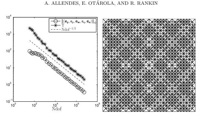
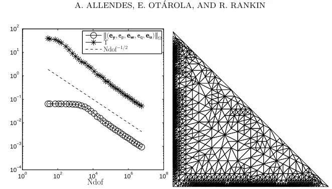
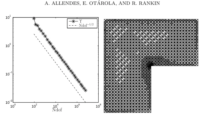
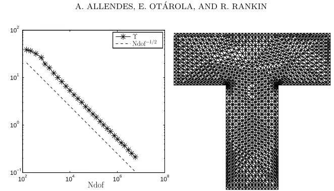
this task we used the adaptive procedure described in Algorithm7.1. We note that the involved estimator Υ provides a guaranteed upper bound on|||(ey,ep,ew,eq,eu)|||Ω.
[image:23.612.107.405.290.364.2]A sequence of adaptively refined meshes was generated from the initial meshes shown in Figure7.1.
Fig. 7.1: The initial meshes used for Examples7.1,7.2,7.3and7.4.
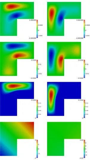
Example 7.1. We consider the square domain Ω = (0,1)2. From [41] we have that (2.14) holds with β = sin(π/8). We tookε = 1, c(x1, x2) = (x2,−x1), κ = 1,
a= (−0.5,−0.5) andb= (0.5,0.5). The dataf andyΩwere chosen to be such that
¯
y(x1, x2) =curl (x1(1−x1)x2(1−x2))2
, ¯p(x1, x2) = cos(2πx1) cos(2πx2),
¯
w(x1, x2) =curl (sin(2πx1) sin(2πx2))2
, ¯q(x1, x2) = sin(2πx1) sin(2πx2).
The results are shown in Figures 7.2and 7.3. We observe that the estimator Υ and the error|||(ey,ep,ew,eq,eu)|||Ωare decreasing at the optimal rate.
Example 7.2. We consider the triangular domain Ω = {(x1, x2) : x1 > 0, x2 >
0, x1+x2 <1}. From [41] we have that (2.14) holds with β = sin(π/16). We took
ε = 0.01, c = (0,0), κ= 1, a = (0,0) and b = (0.1,0.1). The data f and yΩ were
chosen to be such that
¯
y(x1, x2) =curl
x1x22(1−x1−x2)2
1−x1−exp(−1100x1)−exp(−100) −exp(−100)
,
¯
p(x1, x2) = cos(2πx2)/1024,
¯
w(x1, x2) =curl
x21x2(1−x1−x2)2
1−x2−exp(−100x2)−exp(−100)
1−exp(−100)
,
and
¯