Smooth and sharp creation of a spherical shell for a (3+1) dimensional quantum field

Smooth and sharp creation of a spherical shell

for a (3 + 1)-dimensional quantum field

Margaret E. Carrington,1,2,*Gabor Kunstatter,2,3,†Jorma Louko,4,‡ and L. J. Zhou1,2,3,5,§

1

Department of Physics, Brandon University, Brandon, Manitoba, R7A 6A9 Canada

2_{Winnipeg Institute for Theoretical Physics, Winnipeg, Manitoba, R3B 2E9 Canada} 3

Department of Physics, University of Winnipeg, Winnipeg, Manitoba, R3B 2E9 Canada

4_{School of Mathematical Sciences, University of Nottingham, Nottingham NG7 2RD, United Kingdom} 5

Department of Physics and Astronomy, University of Manitoba, Winnipeg, Manitoba, R3T 2N2 Canada

(Received 23 May 2018; published 19 July 2018)

We study the creation of a spherical, finite radius source for a quantized massless scalar field in3þ1 dimensions. The goal is to model the breakdown of correlations that has been proposed to occur at the horizon of an evaporating black hole. We do this by introducing at fixed radiusr¼aa one parameter family of self-adjoint extensions of the three dimensional Laplacian operator that interpolate between the condition that the values and the derivatives on the two sides ofr¼acoincide fort≤0(no wall) and the two-sided Dirichlet boundary condition fort≥1=λ(fully-developed wall). Creation of the shell produces null, spherical pulses of energy on either side of the shell, one ingoing and the other outgoing. The renormalized energy densityhT00idiverges to positive infinity in the outgoing energy pulse, just outside the light cone of the fully-formed wall att¼1=λ. Unlike in the3þ1point source creation, there is no persistent memory cloud of energy. As in the creation of a1þ1 dimensional wall, the response of an Unruh-DeWitt detector in the post-shell region is independent of the time scale for shell formation and is finite. The latter property casts doubt on the efficacy of this mechanism for firewall creation.

DOI:10.1103/PhysRevD.98.024035

I. INTRODUCTION

It has been more than thirty years since Hawking first suggested[1]that black hole formation might give rise to a fundamental breakdown of predictability. Many approaches have been taken in order to resolve this apparent dilemma

[2]. Among these is the suggestion[3–6]that the horizon of a radiating black hole might be more singular than suggested by standard quantum field theory on a curved background

[7,8]. Specifically, there might exist an“energetic curtain”

[5]or“firewall”[6]whose purpose is to break correlations between objects falling into the horizon and those remaining on the outside. An important question then is whether there exists a local mechanism for creating such a firewall, one that does not rely on a detailed knowledge of the underlying theory of quantum gravity.

Recently Brown and Louko[9]explored a1þ1 dimen-sional model of firewall creation based on the imposition of time dependent boundary conditions at a fixed point in space. These boundary conditions were equivalent to the insertion of a wall that broke correlations between the quantum field on the left side of the wall and that on

the right. They found that in the rapid creation limit this scenario resulted in the creation of a divergent null pulse of energy emanating from the point at which the boundary conditions were imposed. It is this pulse of energy that plays the role of the firewall in this model because in the spacetime of an evaporating black hole, the firewall is supposed to be forming near the horizon, which is a null surface. Brown and Louko[9]found that the response of an Unruh-DeWitt detector crossing this pulse remained finite, irrespective of how rapidly the wall was created, suggesting that this mechanism could not produce sufficient energy to break all correlations as required.

A potentially more realistic 3þ1 dimensional model was studied in [10], where time dependent boundary conditions interpolating between Neumann-type (ordinary Minkowski dynamics) and Dirichlet-type were imposed at the spatial origin. This corresponds to the smooth creation of a point source, as opposed to a wall separating two regions of space. As one might expect from standard quantum field theory, the field’s energy and the detector response are more divergent in 3þ1 dimensions than in 1þ1dimensions. The3þ1renormalized energy density hT₀₀iwas shown to be well defined everywhere away from the source but unbounded both above (after) and below (before) the energetic pulse. Moreover, in this model a cloud of positive energy lingers near the source after the

source is fully formed. The total energy of this cloud is positive infinity. At fixed radius,r,hT₀₀iis not static and diverges as t→∞. In the limit of rapid source creation hT₀₀i diverges everywhere in the timelike future of the creation event. The response of an Unruh-DeWitt detector traversing the shell is divergent as desired for the firewall mechanism, but the divergence appears to be primarily due to the energetic cloud that surrounds the source.

The purpose of the present work is to extend the study of this mechanism further by considering the creation of a spherical wall in 3þ1 dimensions. We do this by intro-ducing at fixed radiusr¼aa one parameter family of self-adjoint extensions of the three dimensional Laplacian operator that interpolate between the condition that the values and the derivatives on the two sides of r¼a coincide for t≤0 (no wall) and the two-sided Dirichlet boundary condition fort≥1=λ(fully-developed wall). As in the previous studies, wall creation produces a null pulse of energy on either side of the shell, one ingoing and the other outgoing. We find that hT₀₀i diverges to positive infinity in the outgoing energy pulse, just outside the light cone of the fully-formed wall at t¼1=λ. Unlike in the 3þ1point source creation, there is no persistent memory cloud of energy. As in the 1þ1 dimensional wall, the response of the detector in the post-shell region is inde-pendent of the time scale1=λand finite, once again casting doubt on the efficacy of this mechanism for breaking all entanglement at black hole horizons.

The paper is organized as follows. In Sec.II, we set up the massless Klein-Gordon equation with the boundary conditions atr¼arequired for shell formation. We solve for the mode functions for time t < a and quantize the field. We restrict to t < a in order to ensure that the ingoing pulse does not have time to reach the origin and re-disperse, thereby simplifying the calculation signifi-cantly. In Sec. III, we discuss the quantized total energy with focus on the energy density in the regions to the “future” of the outgoing pulses. A discussion of the energy density in the intermediate regions can be found in Appendix D. Section IV investigates the response of an Unruh-DeWitt detector. Section V concludes with a summary of the results and conclusions. Technical details are given in five Appendices.

II. QUANTIZATION

We consider a real massless scalar field ϕ in (3þ1 )-dimensional Minkowski spacetime with field equation

ð∂2

t −∇2Þϕ¼0: ð2:1Þ

In spherical coordinates, the Laplacian is

∇2_¼ 1 r2∂rðr

2_{∂rÞ þ} 1 r2∇

2

S2 ð2:2Þ

where ∇2_S2 is the Laplacian on the unit S2 sphere. We

consider only the spherically symmetric sector and there-fore we define

ϕ¼fðt; rffiffiffiffiffiffiÞ

4π p

r; ð2:3Þ

so that the field equation(2.1)becomes

ð∂2

t −∂2rÞfðt; rÞ ¼0: ð2:4Þ

We want to consider the formation of a wall, or spherical shell, at positionr¼abetween timest¼0andt¼1=λ. In order to do this, we replace the Laplacian with a one parameter family of self-adjoint extensions defined on L₂ðR3Þ with the sphere at r¼a removed. Some details are given in Appendix A; we summarize the important points below. The self-adjoint extensions of the Laplacian are parametrized by the functionθðtÞ, and we assumeθ∈ ½0;π=2so that the spectrum of the self adjoint extensions of the Klein-Gordon equation has no tachyonic modes. The angle θðtÞ can be written in terms of a function h of a dimensionless variable T¼λt which is defined by the equation

θðtÞ ¼cot−1½LλcotðhðλtÞÞ: ð2:5Þ

L is a positive constant of dimension length which is introduced for convenience; its length is considered fixed. The real solutions of the Klein-Gordon operator satisfy the boundary conditions

fðt;0Þ ¼0 ð2:6Þ

fðt; a−Þ ¼fðt; aþÞ; ð2:7Þ

f0ðt; aþÞ fðt; aþ_Þ−

f0ðt; a−Þ

fðt; a−_Þ ¼2λcotðhðλtÞÞ: ð2:8Þ

In order to model the creation of a shell at r¼a we choose a smooth functionhðTÞ that interpolates between hð0Þ ¼π=2 andhð1Þ ¼0

hðTÞ ¼π=2 forT≤0; ð2:9aÞ

0< hðTÞ<π=2 for0< T <1; ð2:9bÞ

hðTÞ ¼0 forT ≥1: ð2:9cÞ

firewall scenario, we would have to show that it produces a pulse of energy, as explained in Sec.III.

We will quantize the scalar field by writing

ϕðt; rÞ ¼

Z _∞

0 ðakϕkðt; rÞ þa

†

kϕkðt; rÞÞdk; ð2:10Þ

or equivalently

fðt; rÞ ¼

Z _∞

0 ðakUkðt; rÞ þa

†

kUkðt; rÞÞdk; ð2:11Þ

where

Ukðt; rÞ ¼

ϕkðt; rÞ

ffiffiffiffiffiffi

4π p

r ; ð2:12Þ

and the annihilation and creation operators have the commutators ½a_k; a†_k0 ¼δðk−k0Þ. The mode functions U_kðt; rÞ will be normalized so that the field and its time derivative have the correct equal-time commutator. The vacuumj0iis the state that is annihilated by alla_k. We work in the radial null coordinatesu≔t−randv≔tþr, and write the field equation (2.1)

∂u∂vf¼0: ð2:13Þ

We construct an ansatz for the mode functions in two regions inside (r < a) and outside (r > a) the shell. We consider the case whena >1=λwhich means that (in units wherec¼1) the timescale for wall formation is less than the distance between the location of the wall and the origin. Physically this means that during the wall formation process only left-movers are modified inside the shell, and only right-movers are modified outside the shell. Our ansatz is

U_kðt; rÞ ¼

8 > > > < > > > :

1

ffiffiffiffiffiffiffiffi

4πk

p ðe−ikv_þE

kðuÞÞ forr > a; 1

ffiffiffiffiffiffiffiffi

4πk

p ðG_kðvÞ−e−iku_{Þ for0< r < a:}

ð2:14Þ

This form ofUksatisfies the Klein-Gordon equation for any choice of the functionsGkðuÞandEkðvÞ. Our goal is to find a solution for these functions so that the boundary conditions

(2.6)–(2.8)are satisfied. Substituting(2.14)into(2.7),(2.8)

we obtain

−e−ikðt−aÞþGkðtþaÞ ¼e−ikðtþaÞþEkðt−aÞ ð2:15aÞ

2λcothðλtÞ ¼−ike

−ikðtþaÞ_−E0 kðt−aÞ e−ikðtþaÞ_þE

kðt−aÞ

−−ike−ikðt−aÞþG0kðtþaÞ

−e−ikðt−aÞ_þG kðtþaÞ

ð2:15bÞ

where the prime indicates differentiation with respect to the argument. To solve(2.15), we use the dimensionless time variableT ¼λtintroduced previously and define the aux-iliary functionBðTÞ

BðTÞ ¼

8 < :

1 forT≤0;

exp

Z _T

0 cotðhðzÞÞdz

for0< T <1: ð2:16Þ

From (2.9) it is easy to see that Bð0Þ ¼1 and that for 0≤T <1,BðTÞis smooth and satisfies

B0ðTÞ

BðTÞ ¼cotðhðTÞÞ: ð2:17Þ

In AppendixBwe show that1=BðTÞand all of its derivatives approach zero asT →1₋, and therefore1=BðTÞis smooth at T¼1, butBðTÞ→∞asT→1₋.

Rearranging (2.15) we obtain first order differential equations for the derivatives ∂tEkðt; aÞ and ∂tGkðt; aÞ. Introducing the additional dimensionless variables K¼ k=λ and A¼aλ, y¼λu and w¼λv, and defining the functionsRKðyÞ ¼EkðuÞ andSKðwÞ ¼GkðvÞwe obtain

RKðyÞ ¼

8 > > < > > :

−e−iKy _{y <−A}

−e−iKy_þ2isinðAKÞ BðyþAÞ

R_yþA

0 e−iKzB0ðzÞdz y∈ð−A;1−AÞ

−e−iKðyþ2AÞ y >1−A

ð2:18Þ

SKðwÞ ¼

8 > > < > > :

e−iKw _{w < A}

e−iKw_þ2isinðAKÞ Bðw−AÞ

R_w−A

0 e−iKzB0ðzÞdz w∈ðA;1þAÞ:

e−iKðw−2AÞ _{w >1þA}

ð2:19Þ

In order to write equations in a more compact form we sometimes use a shorthand notation in which functions that depend only onyþAare written without their arguments, for exampleB≔BðyþAÞ. This notation is used through-out the Appendices.

The solutions in Eqs.(2.18), (2.19)have the following features:

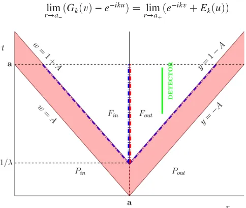
(1) The regions in Fig. 1 marked Pout and Pin

corre-spond to the early time regions, relative to the

wall creation. The top line of either (2.18) or

(2.19) gives the mode functions in these regions, which are just those of the Minkowski vac-uum:Ukðt; rÞ ¼pffiffiffiffiffiffi₄1_πkðe−ikv−e−ikuÞ ¼−

ie−ikt_sinðkrÞ ffiffiffiffi

πk

p .

(2) The regions in Fig.1markedF_outandF_incorrespond to the late time regions, relative to the wall creation. The mode functions in these two regions are obtained from the bottom lines of(2.18),(2.19)which give

Ukðt; rÞ ¼

−ie−ikðtþaÞ_{sin½kðr−aÞ}

ffiffiffiffiffi

πk

p ; y >1−A and r > a½regionFout;

U_kðt; rÞ ¼−ie

−ikðt−aÞ_{sin½kðr−aÞ}

ffiffiffiffiffi

πk

p ; w >1þA and r < a½regionF_in:

Comparing with the above expression we see that when ka¼2nπ, which means that wall formation occurs at a node of the original mode, the mode function in the late time region is the same as the original Minkowski mode.

(3) The middle lines of (2.18) and (2.19) give, respec-tively, the expressions for the mode functions on the inward and outward light cones of the events where the boundary condition changes [atr¼aandt∈ð0;λ−1Þ]. (4) For t < a we have

lim r→a−ð

GkðvÞ−e−ikuÞ ¼ lim r→aþð

e−ikv_þE kðuÞÞ

and therefore the mode functionsUkðt; rÞ are con-tinuous at the location of the shellr¼a.

(5) It is easy to see thatRKðyÞis smooth fory <1−A and in AppendixB we show that it is also smooth at y¼1−A. Similarly SKðwÞ is smooth for w≤1þA.

(6) The mode functions are normalized so that

ðϕk;ϕk0Þ ¼i

Z _∞

0 drr 2Z

S2

dΩðϕk∂tϕk0−ð∂tϕkÞϕk0Þ

¼δðk−k0Þ

for any constant time hypersurface witht <λ−1. (7) The late time region inside the shell (w >1þAand

r < awhich is denoted regionFin in Fig.1) is not

part of our calculation. One problem is that this part of the spacetime diagram would be influenced by waves reflected at the origin, so that we do not expect the ansatz(2.14)to be satisfied in this region. Physically, once the shell is fully formed, an infinite potential separates the regions inside and outside, which means there is no flow of probability be-tween them.

Useful alternate expressions for the functions RKðyÞ and SKðwÞare obtained by integrating the middle lines in(2.18) and(2.19)by parts:

R_KðyÞ ¼−e−iKðyþ2AÞ₋2isinðAKÞ BðyþAÞ

−2KsinðAKÞ

BðyþAÞ

Z _yþA

0 e

−iKz_{BðzÞdz; ð2:20Þ}

SKðwÞ ¼e−iKðw−2AÞ−

2isinðAKÞ Bðw−AÞ

−2KsinðAKÞ

Bðw−AÞ

Z _w−A

0 e

−iKz_{BðzÞdz: ð2:21Þ} FIG. 1. Spacetime diagram of the evolving boundary

condi-tions. The interpolation between θ¼π=2 and θ¼0 at r¼a

occurs over0< t <λ−1, and the null cones of the events where the boundary condition changes fill the regionsð−A < y <1− A; r > aÞ and ðA < w <1þA; r < aÞ in the spacetime. The triangular regions markedPout,Pin,Foutand Finindicate what

We note that the mode functions in the future regions Fin

and Fout, from the third lines of (2.18) and (2.19), areλ

independent. As we will see in the Sec.IV, this means that the detector response in the future regions does not depend onλ, which is the parameter that controls how fast the shell evolves atr¼a.

III. TOTAL ENERGY

The expression for the energy density outside of the shell in terms of the mode functionsR_KðyÞhas exactly the same form as in Ref.[10]. We summarize the calculation and give the result below. The renormalized energy density of the quantized field in the statej0iis obtained by point-splitting the field operators, taking the expectation value in j0i, subtracting the corresponding expectation value in the Minkowski vacuumj0iM, and taking the coincidence limit. This gives

hT₀₀i ¼ h0jT₀₀j0i_ren ¼_ulim

1;u₂→u v₁;v₂→v

ð∂u1∂u2þ∂v1∂v2Þ

×½h0jϕð1Þϕð2Þj0i−h0_Mjϕð1Þϕð2Þj0_Mi

¼ 1 4π

hð∂ufÞ2i r2 þ

hfð∂uf−∂vfÞi þc:c

2r3 þ

hf2i 2r4

:

ð3:1Þ

Using Eq.(2.11)and the first line of(2.14)we obtain in the outside region (r > a)

hT₀₀i ¼ λ 2 16π2_r2

Z _∞

0 dK

K ½jR

0

KðyÞj2−K2

− 1

32π2_r2

∂ ∂r

Goutðt; rÞ

r

ð3:2Þ

where G_out is defined as

Gout¼

Z _∞

0 dK

K ½je

−iKw_þR

KðyÞj2−je−iKw−e−iKyj2:

ð3:3Þ

Using the second line of(2.14)gives for the inside region (r < a)

hT₀₀i ¼ λ 2 16π2_r2

Z _∞

0 dK

K ½jS

0

KðwÞj2−K2

− 1

32π2_r2

∂ ∂r

Ginðt; rÞ

r

ð3:4Þ

with the definition

Gin¼

Z _∞

0 dK

K ½jSKðwÞ−e

−iKy_j2_−je−iKw_−e−iKy_j2_{: ð3:5Þ}

In the early time regions, which are denotedPoutandPin

in Fig.1,hT₀₀ivanishes by construction. In the late time regions Fout and Fin, the first terms in (3.2) and (3.4)

vanish, as can be seen from(2.18), (2.19). The functions Gout andGin are easily calculated. We obtain

Gout future¼Gin future ¼ln½ðr−aÞ2−lnðr2Þ ð3:6Þ

hT₀₀i_future¼ 1

16π2_r4ðlnjr−aj−lnðrÞÞ− 1 16π2_r3

1 r−a−

1 r

:

ð3:7Þ

This result shows that the energy density goes discontinu-ously from positive infinity just inside the shell to negative infinity energy just outside the shell. However, the spatial integral of the energy density along a constant time hyper-surface which crosses r¼a produces a finite energy, if interpreted at r¼a in the principal value sense. In AppendixD we consider the intermediate outside region r > aand−A < y <1−Aand consider the continuity of the energy density asyþA→1−. We show that the energy density is finite everywhere except to the immediate past of the light cone of the point where boundary condition finishes changing, where it is positively divergent.

IV. DETECTOR RESPONSE

In this section we consider an inertial Unruh-DeWitt (UDW) detector [11,12] that is linearly coupled to the quantum field and at a fixed spatial location. Using first-order perturbation theory, the probability that the detector undergoes a transition from a state with energy 0 to a state with energy ω is proportional to the response function

[7,8,11,12]

FðωÞ ¼

Z _∞

−∞dt1

Z _∞

−∞dt2e

−iωðt1−t2Þχð_t1Þχð_t2ÞWð_{t1; t2}Þ_;

ð4:1Þ

where the smooth real-valued switching functionχ spec-ifies how the detector’s interaction with the field is turned on and off, and W is the pull-back of the field’s Wightman function to the detector’s worldline. We consider a detector located outside the spherical shell (r > a) and operating only in the future regiony >1−A. The response function is

ΔFðωÞ ¼

Z _∞

−∞dt1

Z _∞

−∞dt2e

−iωðt1−t2Þχð_t

1Þχðt2ÞΔWðt1; t2Þ;

ð4:2Þ

ΔWðt₁; t₂Þ ¼ 1 4πr2

Z _∞

0 ðUkðt1−r; t1þrÞUkðt2−r; t2þrÞ

−UM

k ðt1−r; t1þrÞUMkðt2−r; t2þrÞÞdk: ð4:3Þ

The functionsUk andUk are obtained from the first line in

(2.14)withE_kðuÞ ¼R_KðyÞandR_KðyÞgiven by the last line of(2.18);UM

k andUMk are obtained in the same way except using the first line of(2.18). Substituting these expressions and collecting terms we find

16π2_r2_ΔWðt 1; t2Þ ¼

Z _∞

0 dk

k ðe

ikð2r−t₁þt₂Þ_þe−ikð2rþt₁−t₂Þ

−eikð2a−2r−t1þt2Þ−_e−ikð2a−2rþt1−t2ÞÞ_:

ð4:4Þ

Doing thekintegral we get

16π2_r2_ΔWðt

1; t2Þ ¼ln

j4ða−rÞ2−ðt₁−t₂Þ2j j4r2−ðt₁−t₂Þ2j

þiπsgnðt₁−t₂Þθðr−jt₁−t₂j=2Þ ×θða−rþ jt₁−t₂j=2Þ: ð4:5Þ

The change in the Wightman function isλindependent, and therefore one does not obtain a divergent response in the limitλ→0, which would correspond to instantaneous wall creation. There is a divergence whenjt₁−t₂j ¼2r, but this divergence is only logarithmic.

V. CONCLUSION

We have extended previous work on firewall creation via time dependent boundary conditions by considering the smooth and sharp creation of a fixed radius shell in (3þ1 )-dimensional Minkowski space. This was implemented by introducing atr¼aa one parameter family of self-adjoint extensions of the three dimensional Laplacian operator that interpolate between the condition that the values and derivatives on the two sides of r¼a coincide for t≤0 (no wall) and the two-sided Dirichlet boundary condition fort≥1=λ(fully-developed wall). Wall creation produces null pulses of energy on either side of the shell, one ingoing and the other outgoing. As in the previous two calculations,

[9,10], the boundary condition is being changed by an external agent whose dynamics is not included in the field action. The total energy of the field hence need not be conserved on its own since the external agent may inject energy into the field. Since we are primarily interested in the detector response across the energy pulse, we have not calculated all the contributions to the field energy on hypersurfaces of constant Minkowski time, in particular the contributions from inside the shell, and therefore have

not established whether the total energy of the field can be unambiguously defined.

We found that the process of shell creation is signifi-cantly more divergent than in (1þ1)-dimensions [9], but less divergent than for point-like source creation in (3þ1 )-dimensions [10]. In the present case, the energy density hT₀₀i diverges to positive infinity in the outgoing energy pulse, just outside the light cone of the fully-formed wall at t¼1=λ. Unlike in the 3þ1 point source creation case, there is no persistent memory cloud of energy. As in the 1þ1dimensional wall case, the response of the detector in the post-shell region is independent of the time scale1=λ and finite, casting doubt once again on the viability of wall creation as a possible mechanism for breaking entangle-ment at the event horizon of an evaporating black hole.

Finally, we note that in order to determine how well breaking correlations by changing boundary conditions models the breaking of correlations in the proposed quantum gravitational firewall scenario, one would need to address the gravitational dynamics. This remains a question for future work.

ACKNOWLEDGMENTS

This work was funded in part by the Natural Sciences and Engineering Research Council of Canada (M. E. C. and G. K.) and by the Science and Technology Facilities Council (JL, Theory Consolidated Grant No. ST/P000703/1). For hospitality, G. K. thanks the University of Nottingham, and J. L. thanks the University of Winnipeg and the Winnipeg Institute for Theoretical Physics.

APPENDIX A: SCALAR LAPLACIAN ONR3

WITH A SPHERICAL SHELL

Defining the short hand notation⨍∞₀dr¼Ra−

0 þ

R_∞

aþand scalingg¼f=r, we can map the 3 dimensional Laplacian and the L₂ inner product on a positive half line with a spherical shell atr¼ato

∇2_⇒∇2_¼∂2

rþ 1 r2∇

2

S2;

ðg₁; g₂Þ⇒ðf₁; f₂Þ ¼

Z

S2 dΩ

⨍

0drf¯1f2: ðA1Þ

We consider only the spherically symmetric case [see Eq.(2.3)], and Hermiticity of∇2 requires

ðf₁;∇2f₂Þ−ð∇2f₁; f₂Þ

¼

⨍

Sðt; xÞ ¼ 1

ð2iLÞðjL∂rf−ifj

2_{−jL∂rfþifj}2_{Þ: ðA3Þ}

Following the method in [13], we find that the boundary conditions are given by

0 B @

Lf0_þ−if_þ

Lf0₋þif₋

Lf0₀−if₀

1 C

A¼U

0 B @

Lf0_þþif_þ

Lf0₋−if₋

Lf0₀þif₀

1 C

A ðA4Þ

where we have used the shorthand notation fðt;0Þ ¼f₀, fðt; a−Þ ¼f₋ and fðt; aþÞ ¼f_þ, and the choice of a unitary 3×3 matrix U specifies the boundary condition. Generally, the matrix U would be decomposed by Gell-Mann matrices. We choose an expression ofUthat ensures no flow of probability through the origin and depends on one free parameter which is a time dependent function chosen to model the formation of the wall atr¼a. We use

U¼

0 B @e−iθðtÞ

cosθðtÞ isinθðtÞ isinθðtÞ cosθðtÞ

1

1 C

A ðA5Þ

and Eq. (A4) gives the conditions

fð0Þ ¼0 ðA6Þ

f₋¼f_þ ðA7Þ

2

LcotθðtÞ ¼ f0_þ f_þ−

f0₋

f₋ ðA8Þ

We note that the continuity of the wave function atr¼ais a result of our choice of UðθÞ, and does not have to be imposed as an extra condition.

APPENDIX B: MODE FUNCTION REGULARITY

In this Appendix we show that the mode functionR_KðyÞ isC26aty¼1−A. We follow closely Appendix B of[10].

1. Smoothness of 1=BðyÞ

First we show that 1=BðyÞand all its derivatives go to zero as y→1₋. We write gðyÞ≔tanðhðyÞÞ and from Eq. (2.9) we see that gðyÞ>0, and gðyÞ and all its derivatives approach 0 as y→1₋.

Using (2.16)we obtain

BðyÞ ¼exp

Z _y

0 dz gðzÞ

ðB1Þ

B0ðyÞ ¼BðyÞ=gðyÞ: ðB2Þ

DefiningB_inðyÞ¼1=BðyÞ, we haveB_in0 ðyÞ ¼−B_inðyÞ=gðyÞ. For n∈N, induction gives

Bð_innÞðyÞ ¼ ð−1Þn_P

nðyÞfnðyÞ; ðB3aÞ

fnðyÞ ¼ BinðyÞ

ðgðyÞÞn; ðB3bÞ

where eachPn is a polynomial ingand its derivatives and PnðyÞ→1asy→1−. We show below thatfnðyÞ→0þas y→1₋, and therefore Bð_innÞðyÞ→0. From(B3b) we have

lnðf_nðyÞÞ ¼−

Z _y

0 dz gðzÞ

1þnlnRyðgðyÞÞ

0gdzðzÞ

: ðB4Þ

Asy→1₋, the first parentheses in(B4)tend to∞, while the second parentheses tend to 1 by l’Hôpital. Hence lnðfnðyÞÞ→−∞ as y→1− and therefore fnðyÞ→0þ asy→1−.

2. Differentiability of RKðyÞ

We make the definitions

JKðyÞ ¼

Z _y

0 BðzÞe

−iKz_{dz ðB5Þ}

FKðyÞ ¼JKðyÞ=BðyÞ ðB6Þ

HKðyÞ ¼JKðyÞ=ðgðyÞBðyÞÞ; ðB7Þ

and rewrite the mode function(2.20)as

R_KðyÞ ¼−e−iKð2AþyÞ₋2isinðAKÞ

B −2KsinðAKÞFKðyþAÞ: ðB8Þ

We will show thatRKðyÞisC26atyþA→1− by showing thatF_KðyÞisC26 asy→1₋. We outline the steps below. (1) Calculate derivativesFð_KnÞðyÞ using(B2)to remove factors ofB0ðyÞ, so that the result does not contain derivatives ofBðyÞ.

(2) Define denðyÞ ¼ BðyÞðgðyÞÞn _{and numðyÞ ¼}

FðnÞ

K ðyÞdenðyÞ. In order to use l’Hôpital n times, calculate numðnÞ_{ðyÞand den}ðnÞ_{ðyÞ, again using(B2)} after taking each derivative.

(3) Define numðnÞ_{ðyÞ ¼ num}ðnÞ_{ðyÞ=BðyÞ and}

denðnÞ_{ðyÞ ¼den}ðnÞ_{ðyÞ=BðyÞand replace all} remain-ing factors ofJKðyÞbyFKðyÞBðyÞ. The limit of the nth derivative ofFðyÞasy→1₋ now has the form

lim y→1−F

ðnÞ_ðyÞl’_⟶Hopitalˆ _lim y→1−

numðnÞ_ðyÞ

denðnÞ_ðyÞ : ðB9Þ

numðnÞðyÞ ¼PðyÞ; denðnÞðyÞ ¼1þQðyÞ

where PðyÞ and QðyÞ are polynomials of gðyÞ and its derivatives,FðyÞ, and factorse−iKy_{, and each term contains} at least one power ofFðyÞorgðjÞ_{ðyÞj∈ð0; nÞ. This means} that bothPðyÞandQðyÞgo to 0 asy→1−. We therefore have from(B9)thatFðyÞisC26aty¼1. We stopped the calculation atn¼26because of limitations of computing time and memory. If the proof extends ton∈N, we would have thatRKðyÞis smooth at y¼1.

APPENDIX C: LEMMA AND CONDITIONS ON g

Lemma C.1.

(i) For a complex-valued function fðy; zÞ that is bounded fory∈½0;1 andz∈½0;1þA, we have

lim yþA→1−

1 BðyþAÞ

Z _yþA

0 BðzÞfðy; zÞdz¼0: ðC1Þ

(ii) If in addition∂yfðy; zÞis bounded fory∈½0;1and z∈½0;1þA, we have

lim yþA→1−∂y

1 BðyþAÞ

Z _yþA

0 BðzÞfðy; zÞdz

¼0:

ðC2Þ

Proof.

(i) By boundedness of f, there is a positive constant Csuch thatjfðy; zÞj≤C. For0< yþA <1, using the triangle inequality and the positivity of B, we have

_Bðy1_þAÞZ yþA

0 BðzÞfðy; zÞdz

≤ C

BðyþAÞ

Z _yþA

0 BðzÞdz: ðC3Þ

When yþA→1, the rightmost expression in(C3)

goes to zero, using l’Hôpital and(B2).

(ii) For0< yþA <1, we expand out the derivative in

(C2)using(B2)and make some cancellation. After repeatedly applying l’Hôpital as yþA→1 and using lemma(C1), the proof is done. ▪ Conditions C.2. We introduce the technical assumption that g000ðyÞ<0for0<y<1. It follows thatg00ðyÞ>0and g0ðyÞ<0for0< y <1. For0< z≤yþA <1, this implies

g0ðzÞ≤gðyþAÞ−gðzÞ yþA−z ≤g

0_{ðyþAÞ; ðC4Þ}

g00ðyþAÞ≤g

0_ðyþAÞ−g0_ðzÞ

yþA−z ≤g

00_{ðzÞ; ðC5Þ}

where the quotients are understood at z¼yþA in the limiting sense.(C4)can be verified by writing the numerator as the integral ofg0 and using the monotonicity ofg0, and

(C5)can be verified similarly be writing the numerator as the integral ofg00. We will derive three consequences which are used in Secs.D 2andD 3.

(i) First consequence: limyþA→1₋g 0_ðyþAÞ

gðyþAÞ ¼−∞. For0< yþA <1, using the monotonicity ofg0, we have

gðyþAÞ ¼−

Z ₁

yþA

g0ðzÞdz≤ −g0ðyþAÞ

×

Z ₁

yþA

dz¼−ð1−y−AÞg0ðyþAÞ:

ðC6Þ

Hence g0ðyþAÞ=gðyþAÞ≤ −1=ð1−y−AÞ, which implies lim_yþA→1−g_g0_ðð_yy_þþ_AA_ÞÞ¼−∞.

(ii) Second consequence:limyþA→1−CðyÞ ¼0 For 0< yþA <1, we define

CðyÞ ¼ 1 BðyþAÞ

Z _yþA

0 dzcosðyþA−zÞB

0_ðzÞ

×gðyþAÞ−gðzÞ

yþA−z ; ðC7Þ

C−ðyÞ ¼ 1 BðyþAÞ

Z _κ

0 dz

gðyþAÞB0ðzÞ yþA−z −

BðzÞ yþA−z

;

ðC8Þ

CþðyÞ ¼_Bðy1_þAÞ

Z _yþA

κ dzB

0_ðzÞgðyþAÞ−gðzÞ

yþA−z ; ðC9Þ

˜

C−ðyÞ ¼− 1 BðyþAÞ

Z _κ

0 dz BðzÞ

yþA−z; ðC10Þ

˜

CþðyÞ ¼_Bðy1_þAÞ

Z _yþA

κ dzB

0_ðzÞg0_{ðzÞ; ðC11Þ}

where 0<cosðyþA−zÞ≤1, B0ðzÞ>0 and g0ðzÞ<0 for 0< z < yþA, and we have intro-duced a constant κ with 0<κ< yþA <1. We haveC˜−ðyÞ<C₋ðyÞandC˜_þðyÞ≤C_þðyÞusing(C4). Therefore

˜

CþðyÞ þC˜−ðyÞ<CþðyÞ þC−ðyÞ<CðyÞ<0 ðC12Þ

As yþA→1−, both integral C˜−ðyÞ and integral

˜

CþðyÞ tend to 0. From (C12) it then follows

(iii) Third consequence: limyþA→1−DðyÞ ¼0 We define

DðyÞ ¼1 B

Z

yþA

κ dzB

0_ðzÞcosðαÞ

α

×

gðAþyÞ−gðzÞ

α −g0ðAþyÞ

; ðC13Þ

D2ðyÞ ¼_B1

Z _yþA

κ dzB

0_ðzÞ1

α

×

gðAþyÞ−gðzÞ

α −g0ðAþyÞ

; ðC14Þ

D3ðyÞ ¼ 1 B

Z

yþA

κ dzB

0_ðzÞ1

αðg0ðzÞ−g0ðAþyÞÞ; ðC15Þ

D4ðyÞ ¼−1 B

Z

yþA

κ dzB

0_ðzÞg00_{ðzÞ; ðC16Þ}

where α≔yþA−z, 0<cosðyþA−zÞ≤1 and B0ðzÞ>0for 0< z < yþA. Using Eqs. (C4)and

(D.2), there is

D4ðyÞ≤D3ðyÞ≤D2ðyÞ<DðyÞ<0: ðC17Þ

Further use of l’Hôpital on D4ðyÞ we find limyþA→1−D4ðyÞ¼0, which means limyþA→1−DðyÞ¼0.

APPENDIX D: BEHAVIOR OF hT00iOUTSIDE

THE SHELL IN THE INTERMEDIATE REGION

In this section we study the behavior of the energy density outside the shell (r > a) in the intermediate region (−A≤y≤1−A), which is given in Eq. (3.2) with the function Gout defined in (3.3), and RKðyÞ given in the middle line of (2.18). We rewrite these expressions as

hT₀₀i ¼ λ 2

16π2_r2½FðyÞ þF˜ðyÞ ðD1Þ

FðyÞ ¼

Z _∞

0 dK

K ½jR

0

KðyÞj2−K2 ðD2Þ

˜

FðyÞ ¼− 1 w−y

∂w−∂y− 2

w−y

Gout; ðD3Þ

where the notation suppresses the dependence ofFðyÞand

˜

FðyÞonw. We comment that the denominators in(D3)are produced by the factor1=rin Eq.(3.2), and the action of the derivative ∂r on this factor.

1. Preliminaries

From(2.20)we have for fixedy∈ð−A;1−AÞthe small K estimates

RKðyÞ ¼−1þOðKÞ; ðD4Þ

jR0_KðyÞj2¼OðK2Þ; ðD5Þ

and the largeK estimates

jR_KðyÞj2¼1þ2B

0

B

sinð2AKÞ K þOðK

−2_{Þ; ðD6Þ}

jR0

KðyÞj2¼K2þ 2B0

B Ksinð2AKÞ þOðK

−1_{Þ: ðD7Þ}

Using these results it is straightforward to show that the integrals in Eqs. (D2) and (D3) are well defined fory∈ð−A;1−AÞ.

At y¼−A both integrands vanish. At y¼1−A the integrand in (D2) vanishes, and a straightforward calcu-lation gives Goutjy¼1−A¼2½lnðr−aÞ−lnr in agreement with(3.6). In the remainder of this Appendix we study the continuity of FðyÞ and F˜ðyÞ in Eqs. (D2) and (D3)

asyþA→1₋.

2. Term FðyÞ

We divide the integral in(D2)into two pieces defined as

F₋ðyÞ ¼

Z ₁

0 dK

K ½jR

0

Kj2−K2; ðD8Þ

F_þðyÞ ¼

Z _∞

1 dK

K ½jR

0

Kj2−K2: ðD9Þ

To show thatF−ðyÞis finite, we use the form ofRKðyÞin Eq. (2.20). Differentiating and substituting into (D8), we get an expression withHKas defined in Eq.(B7)andfi≔ f_iðyþAÞas defined in Eq.(B3b). It is then straightforward to show with l’Hôpital that lim_yþA→1−F₋ðyÞ exists and is finite.

Now we study the second termF_þðyÞ. Our strategy is as follows:

(1) Integrate by parts inz, taking the antiderivative of the factor eiKz, until we have enough powers of 1=K so that theK-integral is convergent.

(2) Switch the order of thezandKintegrals and do the K integral.

(3) Integrate by parts again so that derivatives are removed from factorsBðzÞ.

(4) Analyse the behavior of the remaining integrals. Defining

VK¼ 1 B

Z _yþA

0 dzB

the result of step (1) is

F_þðyÞ ¼

Z _∞

1 dK

4VKVKsin2ðAKÞ K3g2 −

4sin2ðAKÞðVKeiKðAþyÞþVKe−iKðAþyÞÞ K3g3 þ

4isin2ðAKÞðVKeiKðAþyÞ−VKe−iKðAþyÞÞ K2g2

þ2isinðAKÞðVKeiKy−VKe−iKyÞ

Kg þ

4sin2_ðAKÞ K3g4 þ

2sinð2AKÞ g

: ðD11Þ

The integral over large K has terms of the form

R_∞

1 dKsinð2AKÞ which is regularized with a factor e−δK to obtain a finite result in the limit δ→0. The other K integrals can be done using

Z _∞

1 dK

K ðe

iKα_þe−iKα_{Þ ¼−2CiðαÞ ðD12Þ}

Z _∞

1 dK K2ðe

iKα_þe−iKα_{Þ ¼2cosðαÞþ2αSiðαÞ−πα ðD13Þ}

Z _∞

1 dK K3ðe

iKα_þe−iKα_{Þ ¼cosðαÞ−αsinðαÞ þα}2_CiðαÞ

ðD14Þ

whereα>0and Ci and Si are the cosine and sine integrals in the notation of[14].

First, for terms that includeVK as defined in(D10), we interchange the integration by the absolute convergence of multiple integral, and we evaluate the integration overKto reach an expression containing elementary functions and expressions like (D12). Many terms would contain factor B0orB00, but we simply integrate by part to reduce them to combinations involving(C1)and(C2).

Next we introduce the parameters α≔Aþy−z, β≔A−yþz, γ≔3Aþy−z, which will be used in 2nd, 3rd and 4th terms of (D11) for which we have z∈ð0; yþAÞ; and ρ≔2A−xþz, σ≔2Aþx−z and τ≔x−zfor the 1st term of (D11)where x∈ð0; yþAÞ andz∈ð0; xÞ. Using our original assumptionA >1these parameters are all positive over the full range of the corresponding integrals. We therefore find out that single integrals not having factors CiðαÞand double integrals not having CiðτÞ can be easily proven to be bounded whenyþA→1₋.

Third, we consider the remaining contributions to(D9)

which contain factors CiðαÞ and CiðτÞ. These are the difficult terms and we label themI_hard. The terms contain-ing CiðτÞare double integrals of variablexandz, we handle them by first integrating by part in z then x and then integrating by part inx thenz. This two different ways of integration by parts generate two equivalent expressions of the double integral. A lot of terms cancel out when we represent the double integral using its two equivalent expres-sions, further use of Lemma C.1, lim_yþA→1−CþðyÞ ¼0and limyþA→1−DþðyÞ ¼0in Appendix C.2 eventually reduce the result to

lim yþA→1−

Ihard¼− lim

yþA→1− g0

g2: ðD15Þ

ThereforeFðyÞis divergent asyþA→1₋.

3. The termF˜ðyÞ

The integral in(D3) can be divided into two pieces

G−

out¼

Z ₁

0 dK

K ½je

−iKw_þR

KðyÞj2−je−iKw−e−iKyj2; ðD16Þ

Gþ

out¼

Z _∞

1 dK

K ½je

−iKw_þR

KðyÞj2−je−iKw−e−iKyj2:

ðD17Þ

We use two different forms for RKðyÞ: in G−out we use

Eq.(2.20), and inGþout we use Eq. (2.18).

First we look at the easy piece (D16). We define the factors

l₁ðzÞ ¼cosðzÞ−1

z ; l2ðzÞ ¼

cosðzÞ−1 z2 þ

sinðzÞ

z ; ðD18Þ

and in addition to the definitions α;β;γ;ρ;σ;τ, we use μ≔2A−z,ν≔2Aþz,ξ≔Aþw−zandχ≔w−z−A. It is straightforward to show that the parameters μ, ν, ξ, andχ are all non-negative for A >1, z∈ð0; yþAÞ and y∈ð−A;1−AÞ. We also note thatl₁ðzÞandl₂ðzÞand their derivatives are bounded on z∈ð0; yþAÞ. Using this notation the result after doing theKintegral can be expressed in compact form, where the integrands can be expressed using factorsl₁ðzÞ; l₁ðαÞ; l₂ðρÞ etc. Further use of results from AppendixB 1, l’Hôpital’s rule and Lemma C.1 renders

lim yþA→1−G

−

out¼ lim

yþA→1−

2ln

w−y−2A w−y

−2Ciðw−y−2AÞ þ2Ciðw−yÞ

: ðD19Þ

Gþ

out¼

2 B

Z _yþA

0 dzB

0_{ðzÞCiðαÞ}

þ2 B

Z _yþA

0 dzB

0_{ðzÞðCiðχÞ−CiðβÞ−CiðξÞÞ}

− 4

B2

Z _yþA

0 dxB

0_ðxÞZ x

0 dzB

0_{ðzÞCiðτÞ}

þ 2 B2

Z _yþA

0 dxB

0_ðxÞZ x

0 dzB

0_{ðzÞðCiðρÞ þCiðσÞÞ:}

ðD20Þ

We pass the lengthy procedures of carefully manipulating the double integrals using Lemma C.1 and l’Hôpital and point out that the nonvanishing terms inGþoutcancel out the

cosine integrals in(D19). Final result is

lim

yþA→1₋Gout¼yþlimA→1₋

2ln

w−y−2A w−y

ðD21Þ

which is in agreement with(3.6).

APPENDIX E: INSIDE REGION

In this section we look at the energy density in the region r < a. The idea is to see if there is a symmetry between the inside and outside regions that would allow us to extract the final result for the inside region from the results we have already calculated which are valid outside the shell. We consider each of the four pieces:F₋,F_þ, G−, and Gþ.

We have already outlined how to calculate Fout

− in the outside region, doing the same calculation in the inside region we find out

Fin

−ðy; wÞjA→−A−Fout− ðy; wÞ ¼0: ðE1Þ Here,Fin

−ðy; wÞjA→−A is the inside expression transformed by making sign change onA→−Aand switchesðy; wÞ→ ðw; yÞ. A similar expression holds for G−_inðw; yÞ through transformationðy; w; AÞ→ðw; y;−AÞ

G−

inðw; yÞjA→−A−G−outðy; wÞ ¼0: ðE2Þ

Defining positive definite variables throughout the inside region

ˆ

α¼−Aþw−z; ˆγ¼Aþw−z; βˆ¼3A−wþz;

ˆ

σ¼2Aþx−z; ρˆ¼2A−xþz;

we transform the inside result again and find

Fin_þðw; yÞj_A→−A−Fout_þ ðy; wÞ ¼imaginary: ðE3Þ

With additional definitionsχˆ ¼Aþy−z, ηˆ¼A−yþz, we obtain

Gþ

inðw; yÞjA→−A−Gþoutðy; wÞ ¼imaginary: ðE4Þ

From Eqs.(E1)–(E4)we see that the energy density inside the shell can be obtained from the outside results by performing the transformationðy; w; AÞ→ðw; y;−AÞand dropping any imaginary parts that are produced.

[1] S. W. Hawking, Breakdown of predictability in gravitational collapse,Phys. Rev. D₁₄, 2460 (1976).

[2] For recent reviews see: D. Marolf, The black hole informa-tion problem: Past, present, and future,Rep. Prog. Phys.80, 092001 (2017); W. G. Unruh and R. M. Wald, Information loss,Rep. Prog. Phys.80, 092002 (2017).

[3] S. D. Mathur, The information paradox: A pedagogical introduction, Classical Quantum Gravity 26, 224001 (2009).

[4] S. D. Mathur, The information paradox and the infall problem,Classical Quantum Gravity28, 125010 (2011). [5] S. L. Braunstein, Black hole entropy as entropy of

entan-glement, or it’s curtains for the equivalence principle, arXiv:0907.1190v1; S. L. Braunstein, S. Pirandola, and K. Źyczkowski, Better Late than Never: Information Retrieval from Black Holes, Phys. Rev. Lett. 110, 101301 (2013).

[6] A. Almheiri, D. Marolf, J. Polchinski, and J. Sully, Black holes: Complementarity or firewalls?,J. High Energy Phys. 02 (2013) 062; A. Almheiri, D. Marolf, J. Polchinski,

D. Stanford, and J. Sully, An apologia for firewalls,J. High Energy Phys. 09 (2013) 018.

[7] N. D. Birrell and P. C. W. Davies, Quantum Fields in Curved Space (Cambridge University Press, Cambridge, England, 1982).

[8] R. M. Wald,Quantum Field Theory in Curved Spacetime and Black Hole Thermodynamics (University of Chicago Press, Chicago, 1994).

[9] E. G. Brown and J. Louko, Smooth and sharp creation of a Dirichlet wall in1þ1quantum field theory: How singular is the sharp creation limit?,J. High Energy Phys. 08 (2015) 061.

[10] L. J. Zhou, M. E. Carrington, G. Kunstatter, and J. Louko, Smooth and sharp creation of a pointlike source for a (3þ1)-dimensional quantum field, Phys. Rev. D 95, 085007 (2017).

[11] W. G. Unruh, Notes on black hole evaporation,Phys. Rev. D

14, 870 (1976).

by S. W. Hawking and W. Israel (Cambridge University Press, Cambridge, England, 1979).

[13] G. Bonneau, J. Faraut, and G. Valent, Self-adjoint exten-sions of operators and the teaching of quantum mechanics, Am. J. Phys.69, 322 (2001).