Evaluation of control for the adjustment of the digital cadastral data base (DCDB)

University of Southern Queensland

Faculty of Engineering and Surveying

Evaluation of control for the adjustment of the

Digital Cadastral Data Base (DCDB)

A dissertation submitted by

Mr Wayne Fenwick

In fulfilment of the requirements of

Courses ENG4111 and 4112 Research Project

towards the degree of

Bachelor of Surveying

ABSTRACT

1. Introduction

Cadastral boundaries are the invisible lines that separate land into individual parcels. The Digital Cadastral Data Base (DCDB) is a graphical representation of the cadastral boundaries held in an electronic form. This data forms a base layer in Graphical Information Systems (GIS) however the lack of spatial accuracy may limit the usefulness of the system.

2. Objective

The aim of this project is to estimate the expected accuracies achievable when adjusting the DCDB by using different methods to collect control points.

3. Method

These points will be collected from aerial photos at two different scales, by using Global Positioning System (GPS) to locate fence corners and to coordinate existing survey marks connected to cadastral boundaries. The control points will be used to constrain the adjustments.

To limit the number of variables only a least squares adjustment method has been selected to adjust the DCDB. Several adjustments have been processed using the control points and these results have then been compared and contrasted to establish differences among the accuracies of the resulting DCDB’s.

4. Conclusion

University of Southern Queensland Faculty of Engineering and Surveying

ENG 4111 & Eng 4112 Research Project

Limitations of Use

The Council of the University of Southern Queensland, its Faculty of Engineering and Surveying, and the staff of the University of Southern Queensland, do not accept any responsibility for the truth, accuracy or completeness of material contained within or associated with this dissertation.

Persons using all or any part of this material do so at their own risk, and not at the risk of the Council of the University of Southern Queensland, its Faculty of Engineering and Surveying, or the staff of the University of Southern Queensland.

This dissertation reports an educational exercise and has no purpose or validity beyond this exercise. The sole purpose of the course pair entitled “Research Project” is to contribute to the overall education within the students chosen degree program. This document, the associated hardware, software, drawings, and other material set out in the associated appendices should not be used for any other purpose: if they are to be used, it is entirely at the risk of the user.

Prof G Baker Dean

Certification

I certify that the ideas, designs and experimental work, results, analyses and conclusions set out in this dissertation are entirely my own effort, except where otherwise indicated and acknowledged.

I further certify that the work is original and has not been previously submitted for assessment in any other course or institution, except where specifically stated.

My Full Name Wayne Edward Fenwick

Student Number: 0011020281

ACKNOWLEDGMENTS

TABLE OF CONTENTS

Contents Page

ABSTRACT i DISCLAIMER ii CERTIFICATION iii ACKNOWLEDGMENTS iv

TABLE OF CONTENTS v

LIST OF FIGURES ix

LIST OF TABLES x

LIST OF ACRONYMS xi

CHAPTER 1 - INTRODUCTION 1

CHAPTER 2 - CONCEPTUAL FRAMEWORK 3

2.1 Introduction 3

2.2 Brief History of Hillgrove 3

2.3 What Is Relativity 4

2.4 Graphical Information Systems 5 2.4.1 The Problem with the DCDB 5 2.4.2 GIS Management (Towards a Solution) 8

2.4.2.1 Schematic Management 8

2.5 GPS Basics 14

2.5.1 GPS Sectors 14

2.5.2 GPS Measurement 15

2.5.3 Differential GPS 15

2.5.4 Models of the Earth 16

2.5.5 Coordinate Systems 17

2.6 Positional Uncertainty 20

2.6.1 History of Measurement 21

2.6.2 Effects of Change 21

2.7 Monument Over Measurement 22

2.8 Aerial Photography 23

2.9 Conclusion 25

CHAPTER 3 - METHODOLOGICAL CONSIDERATIONS 26

3.1 Introduction 26

3.2 Traditional Survey 26

3.3 Global Positioning System (GPS) Survey 26

3.4 The Adjustments 27

3.4.1 Adjustment Options 28

3.4.2 Least Squares 29

3.5 Conclusion 30

CHAPTER 4 – METHODOLOGY 31

4.2 Establishing Control 31 4.3 The Least Squares Adjustment 33 4.4 Control by Aerial Photography 36 4.5 Control by GPS Survey of Occupations 37 4.6 Control by Existing Survey 38

4.7 Conclusion 39

CHAPTER 5 – RESULTS 40

5.1 Introduction 40

5.1.1 One Point and Azimuth 40

5.1.2 Multi Point 1:8,000 Aerial Photo 41 5.1.3 Multi Point 1:25,000 Aerial Photo 41 5.1.4 Multi Point GPS Occupations 42 5.1.5 Multi Point GPS Existing Survey Marks 42 5.1.6 Coordination of Permanent Marks 43

5.1.7 Combined Results 44

5.2 Conclusion 44

CHAPTER 6 – COMPARISIONS 45

6.1 Introduction 45

6.2 1PtAz Adjustment 45

6.3 Current Occupations 46

6.4 Multi Point GPS Occ’s 46

6.6 Multi Point 1:25,000 Occ’s 47

6.7 GPS Coordination of PM’s 48

6.8 Conclusion 48

CHAPTER 7 – CONCLUSIONS 50

7.1 Further Work 51

Appendix A - Project Specification 53

Appendix B - Havoc Input File 55

Appendix C - Example of an 1880’s Portion Plan 57 Appendix D - Block Layout and Numbering System 59

Appendix E - Observed Data 68

Appendix F - Results of Adjustments 82 Appendix G - Reduction of PM Observations 87 Appendix H - Comparison of Results in Detail 93

LIST OF FIGURES

Number Title

Page

2.1 The Current DCDB against an Orthorectified Georeferenced Image 8 2.2 Before Subdivision (Schematic Approach) 9 2.3 After Subdivision (Schematic Approach) 10 2.4 Stage 1 Before Subdivision (Topological Approach) 11 2.5 Stage 2 (Topological Approach) 12 2.6 Stage 3 End Result (Topological Approach) 12

2.7 Boundary Over Manhole 13

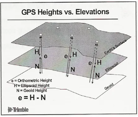
2.8 Relationship between Models of Earth (Trimble 2004, P. 20) 16 2.9 Diagram of UTM (USQ 2003, P. 6.4) 17 2.10 Australian Zones (USQ 2003, P. 6.3) 19 2.11 Reduction of Distances to the Ellipsoid (USQ 2003, P. 8) 20 2.12 Misrepresentation of a Tower (TAFE 1989, P. 106) 25

3.1 Residuals of a Triangle 29

4.1 Plan of Survey Marks used for Primary Control 32

4.2 Plan of PM’s in Hillgrove 33

LIST OF TABLES

Number Title

Page

5.1 1PtAz Statistics 40

5.2 Multi-Point 1:8000 Statistics 41 5.3 Multi-Point 1:25000 Statistics 42 5.4 Multi-Point GPS Occ’s Statistics 43 5.5 Multi-Point GPS Existing Survey Statistics 43 5.6 Permanent Marks Coordinated 43 5.7 Results Compared to Survey Adjustment 44

6.1 1PtAz Comparisons 45

6.2 Current Occupations 46

LIST OF ACRONYMS

ADC Armidale Dumaresq Council AGD66 Australian Geodetic Datum 1966 AHD Australian Height Datum AMG Australian Map Grid

ANS Australian National Spheroid DCDB Digital Cadastral Data Base

DP Deposited Plan

EDM Electronic Distance Measurement GDA94 Geodetic Datum of Australia 1994 GIN Galvanised Iron Nail GIS Geographical Information System GPS Global Positioning System

HAVOC Horizontal Adjustment by Variation Of Coordinates ISG Integrated Survey Grid

LEP Local Environment Plan MGA Map Grid of Australia Occ’s Occupation

PM Permanent Mark

RTK Real Time Kinematic

SCIMS Survey Control Information Management System SSM State Survey Mark

SV Space Vehicle

Trig Trigonometrical Station UHF Ultra High Frequency

CHAPTER 1

INTRODUCTION

The advent of Geographical Information Systems (GIS) has allowed the day to day use of the Digital Cadastral Data Base (DCDB) as a base layer to give spatial meaning and reference to other information. While this has been immensely useful, like so many advances in technology, by solving one problem it has created another. The initial DCDB was captured within both economic and historic technical constraints, therefore restricting the applications for which it can be subsequently used. This has lead to the need to improve the accuracy of the DCDB to enhance its usability and therefore confidence in the product. The problem created is one of how to manage an evolving and shifting DCDB.

There are many approaches to solving this problem such as schematic management, topological management and best estimate management techniques, however, this project will concentrate on evaluating those methods of collecting control points to adjust the DCDB which are driven by the management processes of the best estimate technique.

The reasoning behind this approach is to adjust it once therefore allowing the evolution to occur in the correct location and gain the maximum benefit from the systems that use the data. By assessing the results of this project it will be possible to determine which method of control point collection will provide the appropriate level of control that is required to achieve the desired accuracy of the DCDB.

Now that the broad aims and methodology have been outlined there is a need to explain these in more detail and to assist in this process a brief outline of the dissertation has been supplied to help with the direction of this paper.

Chapter 2 presents the Conceptual Framework underpinning the dissertation and is devoted to setting out the concepts that are needed to appreciate both the problem being researched and the analysis of the data gathered. It will elaborate on the management techniques for GIS and define the problems caused by an evolving DCDB. It will also include a review of literature reporting any previous work pertinent to this project.

Chapters 3 and 4 present a review of the methodological options available to the project to proceed and outlines why the adopted methods were selected, followed by a discussion about the Methodology and the detail behind each method. This will rely on an understanding of the limitations and required processes explained in the conceptual framework.

Chapters 5 and 6 presents a review of the Results will lead to a more detailed discussion about the Comparisons that were able to be made from the analysis of data that were collected.

CHAPTER 2

Conceptual Framework

2.1

I

It is important to have an appreciation of the history in the area that the study has taken place as this has an effect on the results. It is also necessary to understand the concept of relativity and how this affects the management of a GIS. Building on this understanding of relativity, the problem of a dynamic DCDB will be discussed in more detail. Included in that discussion will be the consideration of the different options for the management of spatial systems which will highlight how each method addresses the problems caused by a dynamic DCDB.

Spatial data can be collected in many ways; the traditional surveying methods being well understood while the Global Positioning System (GPS) may require some basic explanation as this is relatively new technology. Another concept is that of positional uncertainty (defined in section 2.6) which, although not a recent idea, is now being recognised as an indication of the quality of spatial data.

Other fundamental background knowledge required to understand the constraints and process used in this project are explored, such as the distortions in aerial photos and the precedent of monument over measurement which is a legal requirement in surveying. This precedent came from English common law and would have been present when the first survey was performed in Hillgrove some 70 years after colonisation.

2.2

B

H

H

unusually high proportion of women and this lead to a very culturally developed society. The town had its own newspaper, Borough Council, Debating Society, Masonic Lodge and recreation ground. (ACC 1994) The electric light came to the town in 1895 from the hydro power station on the Gara River. (NPWS 1994) Hillgrove started to decline from 1900. This is evident as many of the major buildings that burnt down were not rebuilt. By the 1920’s the majority of the remaining buildings had been relocated to Armidale and the surrounding area. (ACC 1994) Today the village has a population of no more than 100 people.

The surveying history is much less detailed. Since the surveys in the 1880’s there is no record of any survey work until recently. There have been three surveys along the southern edge of the village between the mid 1980’s to the early 1990’s and none in the northern part of the village. Coincidently this is about the time that the DCDB was created and started to be used in GIS.

2.3

W

I

R

What is meant by the word relative and the concept of relativity? Why is this important to this discussion? The significance of relativity to this discussion is due to the need manage geographical data in a system and the question arises, if an object moves for some reason how should this affect any of the surrounding objects. The immediate and obvious point in case is, if the DCDB could move as a result of an adjustment how will this affect the other objects in the GIS? This question will lead to considering geographical management techniques and why an object might move. These points will be covered in more detail later in the discussion.

The Australian Concise Oxford Dictionary states that relativity is the fact of being relative and relative is having reference or relating. So from this there can be two arguments put forward. In the context of this discussion these arguments are to be relative to a neighbouring object, which could be described as local relativity, or alternatively to be relative to a central point, which could be described as global relativity.

which direction the car is facing all of the wheels are in the same relative position to each other. The application of this concept will be explored further in the management techniques of GIS.

In contrast, the concept of global relativity is where all points are relative to one fixed point, in both distance and direction, outside the immediate area of concern. An example of this could be the use of GPS. This is where, for all intents and purposes, an object is located and its position is unique within the system and if something nearby should move then it has no affect on the position of the original point.

The two views above can be seen to be contradicting by trying to be different, however, they can also be seen to be saying the same thing, just in two different ways. The key point from this discussion that needs to be clear is that there are two ways to view relativity and neither is wrong, however in GIS the approach adopted will affect the usefulness of the system. To explain a little more about the global approach a few fundamentals of GPS will be explored after the problem caused in GIS by a moving DCDB has been considered in more depth.

2.4

G

I

S

A GIS is made up of many layers of data, for example there could be a roads layer, rivers and creeks layers, a railway layer and utilities layers (water, sewer, stormwater, gas, electricity, etc). There are also layers that are not physical features, such as a historical sites layer or contaminated land layer or archaeological sensitive areas layer, all of which can be known as constraints layers. In a GIS, each layer can be turned on or off as desired. The DCDB is the base layer in a GIS that allows a user of the system to see the relationship of the utility or constraint to the adjacent properties.

2.4.1

The Problem with the DCDB

lead to the engagement of eight contractors, all collecting data. The result was a complete DCDB that was inevitably inaccurate though useable. (Effenberg 2001) In the early systems this was a big step forward as it allowed mapping to occur and data to be collected and placed adjacent to the appropriate parcel.

While being able to locate objects adjacent to the correct parcel is a very valuable tool, problems can emerge when data is collected by a more accurate methods, such as GPS observations, leading to the exposure of inaccuracies within the existing DCDB. This leads to questions of how can the system be improved so that it can be used both more confidently and in more situations. The obvious answer is to increase the accuracy of the DCDB, but the implication of doing this is that all the data placed adjacent to the original DCDB will almost certainly create inconsistencies between layers due to the shifts applied. There is an argument for redrawing the whole DCDB from plans as simply manipulating the existing DCDB into a tightened frame will not remove the errors within the individual blocks. These errors can be as large as 500% in short lines. (An example found in Hillgrove.) In addition there is the consideration of whether or not the data will be moved once or whether the DCDB is to become a dynamic, continually improving dataset. If the dataset is to be continually improving, then how is it possible to maintain the relationships with all the other objects in the system? Many of the datasets within the GIS use the boundaries of the DCDB as a definition of a boundary, an example of this being the Local Environment Plan (LEP). This dataset uses the boundaries of the DCDB to define the shapes in the LEP to a large extent. If the DCDB should move then the LEP needs to move relative to the DCDB to maintain the correct relationship. Another example could be the location of a water service connection. This example will be used to describe the various methods that could be used to manage a GIS.

the development of a fully survey accurate spatial database forming a basis for the spatial integration management and use of land based data – a truly multipurpose cadastre. (Bevin 1999, P. 11)

To highlight the associated problem arising from such a development, an article about Spatial Data Infrastructure (Spencer 2004) points out that some authorities will relocate DCDB boundaries without regard for how this affects other utilities that use the data for their own mapping requirements, causing additional work for the utility agencies. Another paper from FIG Working Week and GSDI-8 (Elfick, Hodson & Wilkinson 2005, P. 1) states that ’The utility of spatial data is greatly improved if it is accurate and consistent between layers, especially given the advent of inexpensive GPS devices’.

Figure 2.1 The Current DCDB against an Orthorectified Georeferenced Image (Reproduced with permission from Armidale Dumaresq Council)

2.4.2

GIS Management (Towards a Solution)

atially inaccurate representation of data and when new spatially accurate data is included it must be made to fit with the existing data, this is achieved by a reduction in accuracy of the new data. This style of GIS does not evolve into a spatially accurate system and is limited in its usefulness. The advantage of this system is data maintains relativity when new data is added to any layer. This management style relies solely on Local Relativity between layers within the system. Some obvious disadvantages are that it is very difficult to share the layers between different GIS’s because the layers in one system may not align to the layers in any There are three main management techniques available to the GIS professional for maintaining its datasets. Each method has its advantages and disadvantages, and these are very subjective depending on what the system is designed to achieve and the background of the people managing the system. Following will be an outline of the Schematic approach, the Topological approach and the Best Estimate approach to GIS management

other system. Also each system needs to maintain the DCDB which creates duplicated effort.

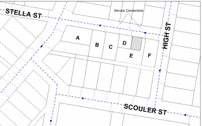
Figure 2.2 and Figure 2.3 are an example of a subdivision of a parcel of land that has been incorporated into the schematic GIS. Note that there is no change in the relationships to the water service connections or the size and shape of any other parcels as a result of the new data being added because of the subdivision of Lot E. The changes that are being ignored in this management technique could be the location of the parcel relative to state survey marks or the size of the adjoining parcel that have been surveyed as part of the subdivision process.

Figure 2.2 is the DCDB before the subdivision takes place. Figure 2.3 is depicting the new DCDB after the subdivision.

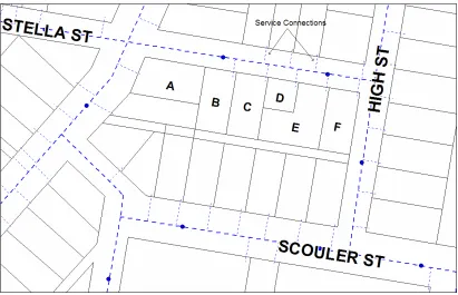
Figure 2.3 After Subdivision (Schematic Approach) (Reproduced with permission from Armidale Dumaresq Council) 2.4.2.2 Topological Management

Another approach is the topologicallycorrect technique. This is an evolutionary style of management that starts with spatially inaccurate data that, over a long period of time, might achieve an acceptable level of spatial accuracy. While this might be a desirable outcome, it is not essential to the approach. Rather, the aim of this method is to maintain the spatial relationships amongst all of the objects stored in each layer and between layers in the system regardless if any of them move for any reason. The sam example of a subdivision of Lot E using this method would result an accurate DCDB

for the lots nts off the

subdivision pla e to be shown

joining to the correct property. This method will be explained in three stages although is one process in practice. Figure 2.4 below is Stage 1 the starting point, the DCDB e

surrounding the subdivision as a result of using measureme n. As well, all the service connections will continu

it

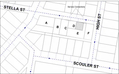
Figure 2.4 Stage 1 Before Subdivision (Topological Approach) (Reproduced with permission from Armidale Dumaresq Council)

Figure 2.5 Stage 2 (Topological Approach) (Reproduced with permission from Armidale Dumaresq Council)

Figure 2.6 Stage 3 End Result (Topological Approach) (Reproduced with permission from Armidale Dumaresq Council)

the GIS manager be sure that all the layers have been amended? That’s a discussion for another paper.

2.4.2.3 Best Estimate Management

The aim of a best estimate GIS is to locate objects so that any movement of the object is not significant within the context of the GIS. This could be achieved by locating all ying standards. That is not to imply, however, that extreme objects to the current surve

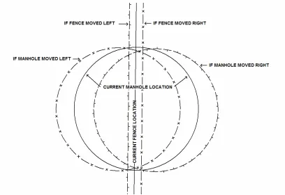
measures need to be taken to locate all objects. For example, there is no need to locate a manhole to the nearest 5 mm, because if a manhole of 1 m diameter is located to the nearest 0.3 m and this manhole is located across the boundary of two parcels which is accurate to the nearest 0.1 m then the boundary could move 0.05 m either way and would still appear to be over the manhole. Figure 2.7 shows the extremes of movement which may occur between the manhole and the boundary.

Figure 2.7 Boundary Over Manhole

an informed decision about the feasibility to supply that service. It may be that it could be too close to call allowing for the known tolerances, in which case more

s used by

e used by the user for planning purposes. The User Sector comprises all the accurate field work would be required. However it could be obvious whether there is, or is not, enough fall to allow the connection.

This level of decision making is not available in any other style of GIS management. By using surveying techniques to collect data such as GPS there is the default acceptance of using the concept of Global Relativity in this management style.

2.5

GPS

B

As stated above use of GPS is ideal for collecting data for GIS applications and will be used in this project to collect control point data. This section will cover some background information relating to the sectors needed for GPS to work, the signal type and their application, this is supplied for completeness and to ensure an understanding of GPS and the jargon used in general discussion. An overview of the model

GPS and for geodetic survey work and coordinate systems. The later two points will be referred to in the section on positional uncertainty.

2.5.1

GPS Sectors

There are three sectors required for GPS to function these are the space sector, the control sector and the user sector. The Space Sector contains all of the Space Vehicles (SV’s) that send out the signals that are received on earth. The Control Sector is made up of five tracking stations that are situated around the equator. These stations monitor and control the SV’s to ensure that they are in the correct position and sending out the correct signals. This sector determines the health of the SV’s and publishes updates that can b

2.5.2

GPS Measurement

All GPS measurements are determined using a ranging technique and there are two different ways that GPS use ranging. One is Code Ranging which only requires one receiver and uses the L1 signal to determine the time and then calculate the position of the receiver. This method only gives a rough estimate of the location. The other method which is used by survey grade GPS receivers involves determining the difference in the carrier phase cycles to calculate the exact number of wavelengths between the antenna and each SV, between two receivers. This method requires both L1and L2 signals to be read and processed and is much more accurate and reliable. The difference between the signals is the frequency that they are transmitted at and the data carried on each signal. (Trimble 2004) While the signal type received may affect the measurement accuracy, the configuration and number of SV’s determines the reliability of the measurements made by the receiver. There is a requirement for a minimum of four SV’s and a PDOP of below 6 before measurement can be taken. PDOP is a value given that relates to the geometry of the SV’s.

2.5.3

Differential GPS

To achieve better accuracy with GPS requires 2 receivers both reading the same

signals roving

receiver just like a radiation measured using traditional surveying techniques. (Trimble

ns to allow a comparison between two radiations. nti ral modes; two have been used in this project. The first mode used for collecting the primary control was Static Survey, this is where two

The second process used to collect secondary control and adjustment points was Real Time Kinematic (RTK), which is where a base receiver is set up on a known point and

from the same SV’s. The result is a reading from the base station to the

2004) This radiation is an unchecked observation and the most common way to check it is to repeat the observation a few hours later when the SV’s are in a different location or have two base statio

Differe al GPS can work in seve

continually tracks the satellites comparing the read position to the known position, calculating a correction factor and then broadcasting this correction via a communication system to the roving receiver. The communication system used in this case was Ultra High Frequency (UHF) radio. The roving receiver receives this broadcast signal and the signals from the same SV’s as the base, applies the correction and so supplies the user with a real time corrected position. (Trimble 2004) While this ethod is far superior to a single unit solution the lack of volume in observed data means that this system is not as accurate however much faster then the static survey method.

To allow GPS to ca , the unit requires

result there are many approximations that have been developed and used m

lculate where the receiver is on the earth’s surface

a model of the earth. There are many models of the earth each with its own advantages. Another name for a model is a Reference Frame.

2.5.4

Models of the Earth

The earth is an irregular shape which is difficult to mathematically define and work with. As a

over the years and one would expect that there are many more to come. An Ellipsoid is an ellipse that is spun through one full rotation on its minor (shortest) axis. A Geoid is the term given to the irregular shape that the earth would be if it were covered with water. This is an equipotential surface formed by the effects of gravity. (Trimble 2004)

To map objects located on the earth’s surface there needs to be some way to represent the curved surface on a flat surface. This can be achieved in many ways such as using projected coordinate systems.

2.5.5

Coordinate Systems

There are many ways to map the earth onto a flat surface. The three major types of coordinates systems are Earth Centred Cartesian Coordinates (X,Y,Z), Longitude, Latitude and Ellipsoidal height and Projection Coordinates. (USQ 2003) All of these rely on a mathematical approximation of the earth being an ellipsoid and some need further manipulation such as the projection coordinates which shall be discussed below in more detail as it is the system used in this project.

Taking one of these models and wrapping a cylinder around one meridian of longitude (see Figure 2.9 below) will allow a projection to be formed. This is known as a Transverse Mercator Projection and a particular method has been adopted world wide with 6 degree wide zones and is know as the Universal Transverse Mercator Projection (UTM).

Each of these projections are named so it is possible to determine which datum is being used or referenced. Examples of these are the World Geocentric Spheroid 1984 (WGS84) used by GPS, Geodetic Datum of Australia 1994 (GDA94) and the Australian Geodetic Datum 1966 (AGD66) which are used for mapping in Australia, and there are many more. However, these three are the relevant models to this

iscussion.

To model the earth’s surface in a small region such as Australia does not mean that the centre of the ellipsoid has to be coincident with the centre of the earth. This is the case

for AGD entre of

D66 datum became the Australian Map Grid (AMG) and that from the GDA94 datum became the Map Grid of Australia (MGA). Figure 2.10 ing data presented in a projection coordinate system there needs to be an awareness of which zone the data is in as the d

66 where the centre of the ellipsoid is approximately 200 m from the c

the earth. This was a deliberate decision to achieve the best possible representation of the earth’s surface over this region.

The result of creating a UTM projection coordinate system allows for the mapping and calculation of distances and bearings on the projection. As there are many ellipsoids there are also many projections and each of these have also been named. For example, the projection from the AG

shows the zones across Australia. When us

coordinate numbers are repeated for each zone, based on a false origin for that zone, to remove any negative numbers. Zones are notated as the projection name followed by the zone number eg MGA 56.

Figure 2.10 Australian Zones (USQ 2003, P. 6.3)

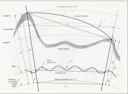
As a result of using GPS to collect the control point data, knowing that this data has been stored as ISG 56/1 coordinates and also knowing that these coordinates are located on the ellipsoid all at the same height, the data from the plans needs to be to a true comparison of distances. The elevation of the reduced the ellipsoid to allow

project site is approximately 1000 m above mean sea level and this means that the distance measured on the ground will be longer than the distance required for the comparison.

Figure 2.11 Reduction of Distances to the Ellipsoid (USQ 2003, P. 8)

The use of GPS has made some surveying tasks much faster by allowing long distances to be measured in a single observation. While all measurements are directly

re lations however,

ents. To this end the

This is a legacy from older measurement systems and in the future measurements taken today will most likely not measu d on a ellipsoid and this avoids the need for reduction calcu

there is still the need to quantify the reliability of the measurem

term Positional Uncertainty is used in surveying and the general concept can be applied to all GIS objects.

2.6

P

U

When measuring a radiation there needs to be a check to ensure no gross error has occurred however there will always be some amount of error as it is not possible to make a perfect measurement. There is a concept that there always some level of error in all measurement and at some point in time that error may be large enough to cause some problem or at least contribute to a problem.

future, need to be aware of the quality of the data they use. Positional uncertainty is a term of acceptance that all measurement is subject to some degree of error. In surveying it is possible to quantify the size of errors and there are tolerances that are regarded as acceptable, at least for the moment.

The current Standard and Practices for Control Surveys known as SP1 defines the term positional uncertainty as;

The uncertainty of the coordinates or height of a point, in metres, at the 95% confidence level, with respect to the defined reference frame. (ICSM 2002, P. xiii)

While this may be applicable for a control survey, a generalisation of the concept is useful also in the context of a GIS. A brief look at the measurement systems used in

millimetre. This is a direct result of gradual improvements in distance measurement ing in links to Electronic Distance Measurement (EDM) and GPS that can measure to millimetres.

ide the surveying profession, that it will facilitate the introduction of a coordinated cadastre and this is believed to be an absolute value. However, these the past will help to explain some reasons why there is less accuracy in older data.

2.6.1

History of Measurement

In the 1400’s the standard of measurement was Rods each Rod is approximately 16.5 feet, in the 1800’s measurements were made in Links each link is 8 inches, then in the 1900’s Inches were used and now Millimetres are a standard unit of measure. As time progresses accuracy increases and what was formerly acceptable is currently no longer acceptable. An example of this are the survey plans in the 1880’s which were drawn with distances shown to the nearest 0.1 of a link (20 mm), then in the early 1900’s plans showed distances to a fraction of an inch (1/8 inch equates to 3 mm) and the current convention is to show distances between control points to the nearest

technology, from the Gunters Chain measur

2.6.2

Effects of change

With the introduction of GPS technology in surveying there may be a belief, both within and outs

conversion from one model to the next may or may not be an exact mathematical conversion. Another factor is the quality of the data; by which method the data was observed and does the data contain accumulated errors. To transform data between the AMG56 and MGA56 projections, both model and quality issues are present. The best method of conversion at present is to use the NT2v Grid which can have errors up to 0.1 of a metre in some areas of New South Wales. (Dr T Watson 2005, pers comm., 21 Oct) A similar process would need to used (although a different grid would be

e significance of this is a GPS measurement using one of the most accurate devices on a fixed station taken in 1994 using WGS84 coordinates

ough the distance on the ground will remain the same as neither mark will have been physically moved. This issue has already been confronted and dealt with from a legal perspective by a historical solution. In surveying there is a precedent that a monument takes dominance over a measurement.

2.7

M

O

M

A monument is defined in The Oxford English Dictionary as any object, natural or artificial, fixed permanently in the soil and referred to in a document as a means of ascertaining the location of a tract of land or any part of its boundaries. It would appear that the prerequisite for converting an object into a monument for the purpose of boundary definition is that the object should be referred to in a document. Hallmann (Hallmann 1973) makes the point that the reference does not need to be a required) to transform data from AGD66 to AGD84 due to the data quality issue, both of these projections are based on the same ellipsoid known as the Australian National Spheroid (ANS).

Further GPS measurements are based on the World Geocentric Spheroid 1984 (WGS84) reference frame. Th

direct reference. An indirect reference such as describing the land by reference to a plan would be enough to allow the plan and all the information in the plan to become part of the document. As a result of this linkage the objects in the plan shown in relation to the boundaries would become monuments.

In cadastral surveying the aim is to redefine the original intention of the survey; that is to mark the same position as the first surveyor. If this was done by pure measurement then with the increase in accuracy over time there would either be slithers of unowned land or disputes of ownership when there is not enough land to fulfil the measurements on the plan. Again the issue of positional uncertainty is present and a key factor in understanding why monuments take precedence over measurements. Historically the legal definition of land has been based on monuments this overcomes the issues of excess and shortage of land as described in plans due to the ability to measure consistently. Objects such as fence posts, brick walls, buildings, trees and survey reference m

objects by measurement and then proportion the available land based on the current measurements to each title to ensure a fair and equitable result based on the original

ion

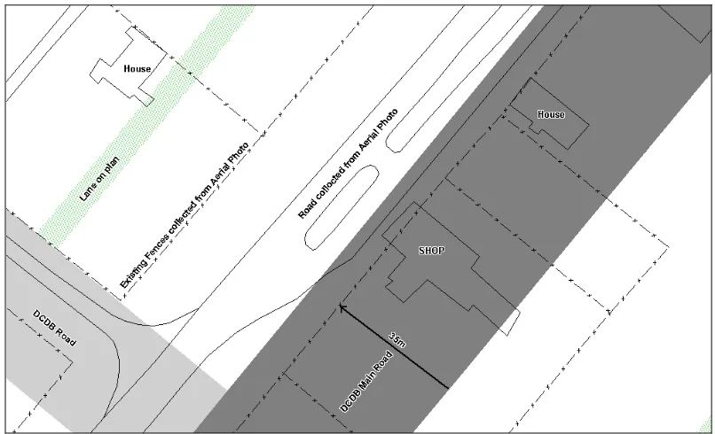
In September 2001, Armidale Dumaresq Council had aerial photography flown and orthorectified (corrected). It was decided to get several scales flown over Hillgrove.

arks become monuments. This allows a surveyor to find and identify these

intent .

The DCDB is a graphical representation of the cadastre at mean sea level and the cadastre is based on monuments to fix corners at the local elevation with these measurements represented on a plan. From the discussion above about ellipsoids as models of the earth’s surface, various projections and the resulting concept of positional uncertainty, it is expected that the values in any DCDB will vary slightly from those shown on its related plans and there will be some level of movement over time. The benefit of having the DCDB connected to monuments is that as measurement technology improves, it is possible to coordinate these and therefore adjust the DCDB to achieve a more accurate model of the cadastre. One method of coordinating these monuments could be the use of aerial photography although this too has some limitations which will be discussed in the next section.

Large scale 1:25,000 photos allowing the detail of the mines workings in the gorge to be seen and the small scale 1:8,000 photos allowed 1 m contours to be created in the village itself.

The scale of th n be obtained

although the limiting factor in this case was the requirement for 1 m contours. A pixel igital image being made up of thousands pixels. The smaller each pixel is the better the quality of the image and the closer it is possible to

see a red or yellow circle on the ground 300 mm in diameter. From the 1:8,000 imagery 0.25 m pixels were created and from the 1:25,000 images

nd terrain elevation can be minimised through orthorectification the misrepresentation of the tree or a building or fence post cannot be

e image creates some limitation on what pixel size ca

is a single square of colour, a d

zoom in to see detail. A pixel resolution described as 0.25 m means that each pixel is 0.25 m x 0.25 m as a ground measurement. As an indication of quality at a pixel size of 0.25 m it is possible to

1 m pixels were obtained.

With such small objects being able to be seen in the photos it is often mistaken for being very accurate. Due to the distortions in an image cause by the lens and the variation in height of the ground it is generally accepted that an image after orthorectification is only accurate to 2.5 times the pixel size. It is also impossible to determine the inaccuracy in an uncorrected image as the errors change constantly in both magnitude and direction.

Due to effects of photography all objects that have height above a selected datum will be displaced. In the image any object such as a tree that both the base and the top can be seen, the result will appear as if the tree is laying flat on the ground except the height of the tree will not be correct and in a radial direction from the centre of the image. The diagram below shows the geometry that causes the effect in the image. While the distortions for lens defects a

Figure 2.12 Misrepresentation of a Tower (TAFE 1989, P. 106)

2.9

C

Hillgrove grew quickly to be an impressive town for its time, however its decline has left a much smaller village and the ravages of time have removed the evidence of any corners marked in the original surveys. As in many rural areas the lack of durable survey marks has meant that little evidence can be found of previous work. Many

mprove their years have passed since that time, though relatively recently a DCDB has been created which has evolved into a dynamic record of land information. These changes have lead to the development of new management techniques to deal with the complexities of topology in GIS. GPS technology has made it possible to locate assets and other objects within acceptable limits of tolerance. All that is left is to improve the accuracy of the DCDB to reduce the effort in managing these systems and to i

CHAPTER 3

Methodological Considerations

e using a total station and reflectors to traverse

would have left behind more marks that could be connected into in the future. The traditional survey methods require closed loops to ensure accuracy and

3.3

G

P

S

(GPS)

S

tion of points. There is the disadvantage of needing a secure place to set up the base station where it will be safe from theft and disturbance either intentional or accidental.

3.1

I

To achieve the aim of this project there were several methods available for collecting the coordinates and adjusting the data. The options considered are outlined and the final choice is justified.

3.2

T

S

A traditional survey would involv

between each of the intermediate stations and would allow several of the points required for coordination to be collected from each intermediate station. This would have been the most accurate method as it is possible to connect to an identified point such as a clout on a fence post. The method would have taken slightly longer in the field although it

quality. An alternative to forming closed loops is to connect onto known points located by another means or from a previous survey. The disadvantage of this is that it is possible to be comparing two surveys of differing accuracy. This makes finding errors much harder. Using this method alone it would be very time consuming to connect into the state survey network.

The RTK GPS survey requires the occupation of each point four times, two from each base station, to ensure that the data collected is of a acceptable quality. If the wrong coordinates are entered into the base the results of a second occupation will appear to the first point collected however once the data from the other base station is collected and compared then it will be obvious that there is a problem. If this should

s required to move all the points and maintain connectivity of the lines. The adjustment of data should only be performed on data that has all of the systematic and

h is the amount by which the traverse does not form a perfect closed figure. Then the misclose distance is divided by the total length of the traverse to give a ratio of accuracy. This ratio is normally stated as 1 in ‘X’ Eg 1 in 8000 or 1:8000 for this discussion 1 in ‘X’ will be used to avoid confusion with photo scales.

There is the assumption that all the plans are of a sufficient standard and the confirm

happen it will mean a complete resurvey of all data collected from that base station. In the case of Hillgrove, there are no marks to check onto to ensure that equipment has been set up correctly. Alternatively if only one observation was collected from each base station it would not be possible to determine which observation was incorrect if they didn’t agree. With the options to collect survey data now considered, the following options are available to adjust the data.

3.4

T

A

The adjustment itself is not a crucial part of this project. In saying that, the adjustment selected i

gross errors removed therefore in an ideal world this process will only be adjusting the random errors within the plans that form the dataset for the adjustment. As this is not and ideal world, unless the error can be isolated beyond reasonable doubt or provided the error is not excessively large, the data will have to be accepted.

When performing a survey it is common practice to determine the accuracy/s of the main traverse routes or loops. This is commonly done by determining the misclose or error whic

would be advantageous to have all boundaries that meant to be parallel, actually being parallel it is not essential provided they are close to parallel.

3.4.1

Adjustment Options

discussed later in this section.

f the DCDB.

Both of the above mentioned methods could be used however neither of the processes much adjustment it has applied to any one line. (Dr T

y the total length of the traverse. This adjustment is then applied to the

IS application MapInfo Professional to shift datasets. After some research it was not possible to determine which adjustment method was used in the application, therefore this is not a suitable solution either.

There are several methods available to perform adjustments, and some of these are outlined in this discussion. The desired adjustment will be able to adjust complex networks and supply a listing of adjusted values of each line in the adjustment. A Helmet Transformation is a four parameter transformation which will scale, shift in X, Shift in Y and rotate the current model. While this may seem adequate this process has some limitations which will be

Rubber Sheeting is a process of stretching the existing dataset between control points on a polynomial approach. For this to be applicable to the DCDB it would require a complete redrafting o

supply any indication of how

Watson 2005 pers comms., 21 Oct) This failing does not supply any indication if a point has been attached to the wrong control point or if anything else has occurred that is undesirable.

The essence of a Bowditch adjustment is a linear adjustment based on the assumption that each line should be adjusted by a proportional amount based on the length of each line divided b

components of each line changing both the distance and the bearing of each line. The Bowditch Adjustment is not applicable as an adjustment method for this project as it will only adjust one traverse at a time and will not deal with complex network adjustments.

An adjustment method which would appear to be adequate is the Least Squares Adjustment method which will be discussed in detail.

3.4.2

Least Square

The main reason to adjust something is to distribute the errors evenly throughout the et. t be gross errors but systematic errors, for example, a gross error would be entering 100.00 when the measurement was 10.00. Alternatively

sea level distances. This reduction of distances is a function of the software not a direct part of the adjustment process.

As a result of using the least squares adjustment process a list of residuals is produced,

s

data s These errors should no

a systematic error could be created by the fact that the instrument only measures to the nearest 5 millimetres and 6 seconds (USQ 2002) or, as in the Hillgrove case, the plans are only quoted to a fraction of a link. If gross errors are adjusted it will corrupt good data and create an unreliable outcome.

Another reason to use an adjustment program is that it is an easy way to convert a large amount of data from the local elevation distances to mean

this is an indication of the amount of movement that occurred in each line. An example of this could be demonstrated by adjusting a 60/30 right triangle that has the lengths of sides of 3.5, 3.75 and 5.75. The correct answer is a 3, 4, 5 triangle because the triangle is constrained by control along the hypotenuse of the length of 5. The residuals would be -0.5, +0.25 and –0.75 respectively. (See Figure 3.1) A residual is the amount of change that needs to be applied to an object to make it fit into the whole network.

The aim of least squares is to minimise the sum of the squares of the residuals. That is to say that the variation to each observation will be a minimum. One advantage of this method is that it adjusts all the observations at the same time. On the other hand to perform a Least Squares adjustment there must be redundant observations. A redundant observation is any observation that is above the minimum number of observations required to solve the problem. This requires extra data collection although the method is able to use direct observation such as those read from an instrument and indirect observation which can be derived from the direct observations. A Frenchman by the name of Adrien Legendre published the principle in 1806. Since that time it has been used to calculate the orbits of planets and many surveying

problems such 2002) It is

possible to use corrupting the

ability to weight observations dependant on the age or reliability of each individual observation and supply a listing of the residuals applied to each line in the

djustment.

The selection of field technique was based on the need to set up the base stations to provide coordinates on the state survey control network to allow Hillgrove to be correctly georeferenced ere time consuming to

get access to so rmed from the

minimum number of setups was to be the most efficient use of time and resources. These restrictions lead to the selection of the GPS for the entire project.

as traverse, GPS levels, resection or intersection. (USQ different datasets that have different accuracies without

good data with poorer quality observation by using weightings to identify the quality of each observation. As all observations are adjusted simultaneously the method lends itself to network adjustments.

An example of this method is the software Horizontal Adjustment by Variation Of Coordinates (HAVOC) supplied by the Department of Lands NSW which has been used in this project.

3.5

C

From the above discussion the adjustment process used is not critical to the project however the least squares method is the most common method employed in the surveying profession to adjust networks and appears to allow the best functionality with its

a

within the DCDB. The base stations w

CHAPTER 4

ary control was brought into Hillgrove for the purpose of suppling photo control for the aerial photos to be flown. This

both high quality horizontal positions and vertical control on the trigonometrical stations (Trig) at Gara Trig and Bora Trig.

hese stations had either no elevation data or poor accuracy data. There was a high precision vertical control survey carried out along Grafton Rd using State Survey Marks (SSM) although none of these marks had horizontal control to an accuracy of better than the nearest 10 metres. This fact made it difficult to locate some of the marks necessitating the identification of substitute marks. Figure 4.1 shows the relative locations of the survey marks used to gain primary control.

METHODOLOGY

4.1

I

In general terms the process used in this project revolves around placing a primary control network and then using that network to control the collection of points of varying reliability to constrain an adjustment based on the survey data for the village. Several variations of control points have been put though the adjustment process. This resulted in many sets of coordinates of varying degrees of accuracy for each corner of each village block. Then a comparison was carried out and conclusions drawn. Each part of this process will be discussed in more detail below.

4.2

E

C

In 2001, using static GPS survey methods prim

process involve using two Ashtech GSR2300 L1/L2 capable GPS receivers, one as a base station set to record continuously from the time it was setup until it was retrieved at the end of each day. The other unit was used as a rover to record 1 hour duration observations on each of the roving stations. Typically there were three roving stations observed twice each day.

There was a complication caused by the lack of

Figure 4.1 Plan of Survey Marks used for Primary Control (Reproduced with permission from Armidale Dumaresq Council)

After the data collection was complete the data was post processed to improve the accuracy of the observations. This was originally carried out by Sokkia Australia located in Sydney. Th station known as B4 located in the Hillgrove Gold and Antimony Mine with accurate Easting, Northing and

the propriety data format of the GSR2300 to Rhinex to allow the Trimble Office Suite to read the data. This allowed the reprocessing of the data to

e outcome of this was the coordination of a

Australian Height Datum (AHD) Elevation also now both Bora Trig and Gara Trig have better quality heights suitable for supplying photo control.

As the use of this data was necessary in this project, the raw observations were converted from

Figure 4.2 Plan of PM’s in Hillgrove

(Reproduced with permission from Armidale Dumaresq Council)

4.3

T

L

S

A

straight forward process of data entry: how wrong could one be! The plans had very few connections across

ierarchy distance was used. Another interesting occurrence was

standard than the plans produced today as there were several cases where the sections

is section closed with accuracies just over The inputting of the data into HAVOC seemed initially to be a

roads although there was a definite road hierarchy with the main roads being 150 links wide and the minor roads being 100 links wide while the lanes were 30.3 links wide. This lent itself to the process of adopting the connection on the plan if one could be found and if not the h

the number of times an angle fell in the road reserve which meant that there was no direct connection available and a close was required to determine the connection across the road. The quality of the plans prepared in the 1880’s were of a lesser

1 in 2000. This was the best data available so a network was constructed by closing each section tying the sections together with connections to each of the neighbouring sections at the corners. An example of the input files and plans can be found in Appendix B and Appendix C respectively.

The software requires a unique naming convention for each point in the adjustment. This required the development of a consistent numbering convention to be devised

o avoid confusion when processing the data in the office. The complete numbering system can be seen in Appendix D.

which left enough space between numbers to add any intermediate points required with out disrupting the numbering system. This was also very useful from a surveying perspective as it was now possible to tag each point collected with the respective number t

Figure 4.3 Example of Numbering System (Reproduced with permission from Armidale Dumaresq Council)

were many adjustments run in this product, each variation with its own strengths or weaknesses.

The one point and azimuth (direction relative to north) (1PtAz) adjustment relies on the selection of one point with reliability as this point will affect the result of the whole adjustment. From this point the program requires an azimuth to orientate the adjustment. The value of this azimuth was determined by a sun observation found on the 1880 village plan and applied the swing to a line in the adjustment. This adjustment had three variations; the first was a point collected from the 1:25,000 scale photo, the second was a control point from the 1:8,000 photo and the last was a GPS

by looking at the aerial photo or by when collecting the post by GPS when there is no other evidence available. Also this adjustment is equivalent to redrawing the DCDB and floating it as located peg.

The advantages of this minimally constrained adjustment are that it identifies that there are no gross errors in the data input for the adjustment as none of the residuals are excessively large. Other advantages are that only one coordinate is required to run the adjustment so it is a good starting point to assess the suitability of those control points obtained by lesser accurate methods such as locating fence posts from aerial photos. An example of this is there is no way to know if a post is on the corner or some distance away from the actual intersection of the boundaries

an uncontaminated estimate of the original intention.

The disadvantage of this adjustment is that it is completely reliant on the two initial values being correct. If either one of these values is wrong, then that result will either be shifted in one direction or swung about the fixed point.

4.4

C

A

P

As noted already, in 2001, ADC flew aerial photography and had it orthorectified to preset targets which were surveyed using an RTK GPS method. This imagery was

1:25,000 imagery.

ethod included the inability to actually see a fence post

Another issue is that an image is apparently only as accurate as 2.5 times the pixel size.

multi-point adjustment to be run with success to achieve results. A separate adjustment was used for the two different scales of photography. This will be covered in more detail during the discussion of the results (see section 5). Another method for the collection of control points was the use of GPS to collect occupations. flown at 1:8,000 and 1:25,000 scales and scanned to provide pixel sizes of 0.25 m and 1.0 m respectively.

Having this data available the selection of control points from each of the images was undertaken independently of each other. That is to say, the values determined from the 1:8,000 imagery had no influence on the values determined from the

The aim of this method was to select fence posts at the corners of the village sections to use as the control for the adjustment. This is based on the assumption that the fence will represent the actual boundary corner.

Problems identified with this m

at these scales, however it was possible to identify the fence lines and where they intersected. Another problem was that vertical objects are displaced in aerial photos due to the angles created from the aircraft, as discussed in section 2.8. This has the effect of potentially picking the wrong point on the image that should represent the base of the fence post and therefore using the wrong value in the adjustment.

This is a rule of thumb accepted in the industry For example a 0.25 m image would have an accuracy of 0.625m. This would obviously limit the results obtained from this method.

4.5

C

GPS

S

O

as made to collect any fence post on the corner of the blocks in the assumption that they would be close. Some blocks only had fencing on one side or

not possible locate where the corner might be. Another block had a splay corner in the fence line where there was no splay in the property boundary so an estimate of where the corner might be was made by lining up the fence lines. The actual surveying process was not as straight forward as was originally thought. The complication was that the GPS antenna is fixed to the top of a 2 m high pole and some of the posts are leaning or have a clout or GIN in them. To take a shot over a clout or leaning post the GPS pole must be lent on an angle and an estimate of when the antenna head is over the mark needs to be made. This is not a repeatable method and as a result there was expected to be some variation in the results. Another restricting variation was that it was not possible to take every shot in the same relative position of the post, such as at the outside edge on the intersection of the two boundaries. This was caused by plants and drainage lines restricting access. These variations were not deemed to be significant in the scheme of the survey although this needs to be considered in the overall accuracy expectations of the project.

As mentioned in the GPS Basics section the limitations of GPS equipment required four shots to be taken at each location to ensure erroneous observations could be removed from the data set before processing. During the processing of these control points for inclusion in the adjustment the same problem with the adjustment failing was found as with the data collected from the aerial photography. The same process was used to cull the control points by comparing them with a 1.5 m variance to the results of a 1PtAz adjustment using a GPS post as the datum point. Typically, this reduced the amount of available control by half and so this improved the result. There is more detail in the discussion about the results.

Collecting control points by using GPS to locate fence posts requires the assumption that the fence post is on the intersection of the boundaries for that parcel. In the case of Hillgrove there has been little survey activity since 1880 and therefore it is very difficult to determine if the post is close to the boundary corner or not. As a result the decision w

4.6

C

E

S

At the point of conceptualisation of this project it was intended to do a complete boundary definition of the area o ional surveying methods. After getting the entire search required for the project and assessing the difficulty of undertaking a full redefinition, and the time this would add to the project against the

st collecting and coordinating existing survey marks, it was decided to do the latter. This will not have a significant effect on the result

s

originally marked. The purpose of this adjustment is to act as the baseline to assess the paring the results.

d was on Bora Trigonometrical Pillar.

e a complete plan search for the area was required in order to assess the likely places that marks till exist. As the majority of the village has not had any survey activity since the 1880`s there was little evidence expected to be found.

Some time was spent on an initial investigation

plans had any pegs still visible. This revealed several pegs in the south west and the south east of the village, however there was dence in the northern part of the village, probably due to the lack of recent work in this part of the town. During the

f interest using tradit

added benefit and accuracy of ju

although the adjustment will not be constrained in the northern section of the village as there are no recent surveys in this area. Given the age of the surveys and the lack of evidence it could be possible that the only way of fixing the boundaries would be to survey the boundaries by dimension from the southern part of the village and see how this fits with the existing fencing. This is effectively the same as putting the bearing and distances in an adjustment, holding the southern part fixed and leaving the northern part floating. Graeme Stewart made a comment that it was possible to spend two weeks doing field work and still not be able to accurately define the corner as

accuracy of the other adjustments by com

This method requires the use of existing survey marks to determine the location of the corners of the DCDB. This was achieved by using RTK GPS to determine the coordinates of the marks. This survey was performed as part of the collection of fence posts and to achieve quality data through four observations at each location. The base stations were located on a station known as B4 in the Hillgrove Gold and Antimony Mine and the other station use

To achieve the desired outcom

might s

to see if any of the three new registered

survey there were several fence posts that had clouts or Galvanised Iron Nails (GIN) in them. As a result of these marks these fence posts were also located.

4.7

C

In general terms the ini rov suitable solution to evaluating the control points for the adjustm DCDB. There was the need for slight modification, in the form g proces e adjustment software was unable to use points that were unreliable and poor es s of the true location of boundary locations.

At point 1020 there was a broad arrow and the number 7 carved into the fence post and there was a peg located 0.5 m away from the post, both of these points were coordinated.

While GPS was chosen as the survey method for this and the previous method, the significant difference between the methods for collecting control points is that this method is connecting to actual cadastral survey marks and the previous method is making the assumption that the fence posts are on the cadastral corners. This difference in collection method is expected to have a profound effect on the accuracy of the end result.

ON

tial methodology p ided a ent of the

CHAPT

5

5.1

I

From that data collected and m

adjustments were processed. This section will review the findings of these y decisions made in those calculations. Each adjustment will be discussed in turn and a summary of the results gathered will

5.1.1

One Point and Azimuth

All of the 1PtAz adjustm e a nt statistics as the only change of the value of the starting e stan eviations used in the adjustment, which act as the weight , were set at 20 seconds for the angles and 2 cm + 20 ppm for the distan ults from djustment show that there are no gross errors in the entere indicated in Table 5.1 by the small size of the Max and Min residual values

ER

RESULTS

TION

anipulated, three PM’s were coordinated and several

calculations and outline the implications of an

allow a comparison to occur. The discussion on these results will occur in Chapter 6. The observed values are available in Appendix E and the results from the adjustments are available in Appendix F. The reduction of the Permanent Marks can be seen in Appendix G. The comparisons to the survey adjustment are located in Appendix H.

ents have the sam djustme coordinate. Th dard d ing mechanism

ces. The res this a d data. This is

Function Value

Average Residual -0.00003

Standard Deviation 0.014

Median Residual 0

Max Residual 0.037

Min Residual -0.048

Range 0.085

Variance 0.701

5.1.2

Multi Point

Aerial Ph

The first adjustment wi l p ollected from the imagery would not run, therefore some ss rel ints was required. The variance adopted was 1.5 m from the results of the min constrained adjustment using the 1:8,000 control point as a starting value. After these points were removed the adjustment ran however with very poor results. The standard deviations were increased to 60 seconds and 100 cm + 100 ppm until a reasonable variance was gained.

There was littl given by 300

seconds (5 minutes) and 500 cm + 500 ppm and a variance of 1.0 at 480 seconds (8 .0 was adopted as the final result. Table 5.2 show the statistics for this adjustment.

1:8,000

oto

th all of the contro oints c culling of the le iable po

imally

e change in the residuals between a variance of 3.7

minutes) and 800 cm + 800 ppm. The variance of 1

Function Value

Average Residual 0.055

Standard Deviation 0.522

Median Residual 0.075

Max Residual 1.584

Min Residual -1.337

Range 2.921

Variance 1.056

Table 5.2 – Multi-Point 1:8000 Statistics

5.1.3

A similar occurrence was experienced with the 1:25,000 imagery derived control points irst adjustm ot run s was culle in 3 m from the 1PtAz adjustment using the 1:25,000 control point value. This adjustment ran su y however eviatio y high a d and 800 cm + 800 ppm. Another adjustment was run after culling the control down within 2 m from the 1PtAz deviations however yielded a similar variance. It was deemed at this point that the results were not going to improve so further variations were not pursued as the limitations of the software are 999 seconds and 999 cm + 999 ppm. Table 5.3 show the statistics for this adjustment.

Multi Point 1:25,000 Aerial Photo

. The