Validation of cooling grid model and testing of alternatives

(1)

University of Southern Queensland

Faculty of Engineering and Surveying

Validation of Cooling Grid Model and

Testing of Alternatives

A dissertation submitted by

Andrew Thomas Watt

in fulfilment of the requirements of

Courses ENG4111 and 4112 Research Project

towards the degree of

Bachelor of Engineering (Agricultural)

(2)

Abstract

The Great Artesian Basin Sustainability Initiative, (GABSI), is a joint state and

federal government project which rehabilitates artesian bores and replaces bore

drains with polyethylene pipeline systems to tanks and troughs for stock water. The

naturally pressurised artesian water can reach temperatures of up to 99˚C due to

the heat convection at great depths within the Earth’s crust. The heated artesian

water is required to be cooled to below 45 ˚C to prevent heat deterioration of the

polyethylene pipe and to maintain a 50 year design life of the entire reticulation

system. Historically, a submerged network of copper pipes has been designed for

each system to provide a cooling mechanism and maintain the natural pressure of

the bore.

The project’s main aim was to predict and confirm the heat transfer parameters for

cooling grids submerged in water and air, investigate alternative cooling options

and validate the design model to accurately reflect existing operation. The testing

procedure utilised a 12 metre length of the three pipe materials under investigation,

which were tested at four representative flow rates surrounded by air and then

submerged underwater. Inlet, outlet, ambient and pond temperatures were

monitored along with relative humidity and weather observations.

The experimental results and research allowed for model to be validated and

deemed accurate with an appropriate factor of safety. The alternative designs

tested were comparatively analysed accounting for costs, cooling performance,

pipeline flow characteristics, material availability, corrosion resistance and

maintenance requirements. Aluminium was determined to exhibit the most

desirable traits and was recommended as the most suitable alternative cooling grid

pipe material. Air as a heat transfer medium was deemed inappropriate for cooling

(3)

(4)

Certification

I certify that the ideas, designs and experimental work, results, analyses and

conclusions set out in this dissertation are entirely my own effort, except where

otherwise indicated and acknowledged.

I further certify that the work is original and has not been previously submitted for

assessment in any other course or institution, except where specifically stated.

Andrew Thomas Watt

Student Number: 0050026431

____________________________________ Signature

(5)

Acknowledgements

Mr Joseph Foley for his supervision, guidance and mentoring, as well as his input

in the project and comments on the dissertation.

Associate Professor David Buttsworth for his supervision and help with the

thermodynamic areas.

Thomas Bean, Simon Orphant and Emile Seiler from the Department of Natural

Resources and Water for their supervision, sponsorship and help during the project

and during testing.

Robert and Sally Hemming, landholders of ‘Beverleigh’ property, Dirranbandi for

(6)

Table of Contents Andrew Watt

3.1 Review of Previous Work

………….. 17

3.2 Heat Transfer Mechanisms

………….. 21

3.2.1 Conduction ………….. 21

3.2.2 Convection ………….. 22

3.2.3 Radiation ………….. 23

3.3.4 Heat Transfer in Cooling Grids ………….. 24

(7)

3.4 Alternative Water Cooling Practices

………….. 26

3.4.1 Gas Refrigeration ………….. 26

3.4.2 Cooling Tanks/Towers ………….. 28

3.4.3 Passive Radiator Cooling Systems ………….. 28

3.4.4 Heat Pipes ………….. 29

3.4.5 Applications to Artesian Bore Water Cooling ………….. 30

3.5 Flow Characteristics in Pipelines

………….. 32

3.6 Pipe Material Selection

………….. 33

Chapter 4: Model Description & Sensitivity Analysis

….. 35

4.1 Model Calculations

………….. 36

4.1.1 User Inputs ………….. 37

4.1.2 Defined Constants ………….. 37

4.1.3 Calculations ………….. 38

4.2 Sensitivity Analysis

………….. 44

Chapter 5: Experimental Methodology

……….. 46

5.1 Field Testing Procedure

………….. 47

5.2 Limitations on Experimentation

………….. 51

5.3 Experimental Design Justification

………….. 52

5.4 Heat Transfer Predictions

………….. 53

Chapter 6: Experimental Results & Model Validation

…. 55

6.1 Heat Transfer Test Results

………….. 56

6.2 Experiment Conditions and Ambient Temperatures

… 60

(8)

Chapter 7: Discussion & Implications

………. 68

7.1 Heat Transfer in Air Tests

…………. 69

7.2 Heat Transfer in Water Tests

…………. 70

7.3 Design Optimisation

…………. 72

7.4 Implications

…………. 74

Chapter 8: Conclusions

……… 76

8.1 Conclusions

………….. 77

8.2 Further Work

………….. 79

List of References

……… 80

Appendix A – Project Specification

………. 82

Appendix B – Spreadsheet Model

……….. 85

Appendix C – Risk Assessment

………... 88

Appendix D – Resources

………... 90

(9)

List of Figures

Figure 1.1 Schematic of Typical Cooling Grid

Figure 2.1: Map of Great Artesian Basin

Figure 2.2: Great Artesian Basin Formation

Figure 2.3 Environmental Problems with Bore Drains

Figure 2.4 Controlled Bore Piped to Tanks

Figure 2.5 Installed Cooling Grid

Figure 2.6 Installed Cooling Grid

Figure 3.1 Gas Absorption System

Figure 3.2 Heat Pipe

Figure 5.1 Air Test Apparatus

Figure 5.2 Data logger and manual readings during pipe in air test

Figure 5.3 Water test apparatus with submerged test material fixed to steel posts

Figure 6.1 Pipe in-air test results indicating inlet and outlet temperatures as well as

the 20 minute regions of varied flowrates for the ALUMINIUM pipe material

Figure 6.2 Pipe in-air test results indicating inlet and outlet temperatures as well as

the 20 minute regions of varied flowrates for the COPPER pipe material

Figure 6.3 Pipe in-air test results indicating inlet and outlet temperatures as well as

the 20 minute regions of varied flowrates for the STAINLESS STEEL pipe material

Figure 6.4 Pipe in-water test results indicating inlet and outlet temperatures as well

as the 20 minute regions of varied flowrates for the ALUMINIUM pipe material

Figure 6.5 Pipe in-water test results indicating inlet and outlet temperatures as well

as the 20 minute regions of varied flowrates for the COPPER pipe material

Figure 6.6 Pipe in-water test results indicating inlet and outlet temperatures as well

as the 20 minute regions of varied flowrates for the STAINLESS STEEL pipe

material

Figure 6.7 The relative error of measured ∆_{T vs modelled}∆_{T at each flowrate for}

(10)

List of Tables

Table 3.1 Typical values of the convection heat transfer coefficient

Table 3.5 Thermal conductivity of some materials

Table 4.1 Sensitivity Analysis Results

Table 6.1a Aluminium Air Test Ambient Temperatures

Table 6.1b Copper Air Test Ambient Temperatures

Table 6.1c Stainless Steel Air Test Ambient Temperatures

Table 6.2a Aluminium Water Test Ambient Pond Temperatures

Table 6.2b Copper Water Test Ambient Pond Temperatures

Table 6.2c Stainless Steel Water Test Ambient Pond Temperatures

Table 6.3 Average Equilibrium Temperatures and Differences

Table 6.4 Measured ∆_T

Table 6.5 Modelled ∆_T

(11)

CHAPTER 1

(12)

Chapter 1: Introduction Andrew Watt

1.0 Introduction

Artesian groundwater flowing to the surface from a 1 to 3 kilometre deep

sandstone aquifer called the Great Artesian Basin, is an important natural resource

and has provided a secure water supply for the settlement and development of

expansive grazing areas throughout western Queensland, north-western New

South Wales, north-east South Australia and the south-east Northern Territory. The

free flowing groundwater can vary in temperature from 30 to 99 ° Celsius at the

surface.

Historically, the water has been distributed across the landscape by gravity through

earthen channels called ‘bore drains’. These extensive man-made networks of

earth channels extend for tens to hundreds of kilometres across pastoral grazing

properties to distribute this artesian water to previously uninhabitable (dry) regions

to produce water stock animals. Without the requirement of cooling, the water has

been allowed to flow uncontrolled under the action of gravity into the bore drain

network which can service up to 200 kilometres from a single outlet. Although the

system is effective in transporting water, the efficiency of water delivery is very low

with as much as 97% of water flowing into the drains being lost to evaporation and

seepage, not to mention the environmental impacts such as weed infestation,

salinity and harbouring of feral animals caused by the drains themselves.

In addition to these high losses, as more bores have been drilled the natural

pressure of the entire basin has dropped significantly, further highlighting the need

for conservation to protect the sustainability of such an important natural resource.

The Great Artesian Basin Sustainability Initiative (GABSI) is a joint federal and

state government project undertaken by the Queensland Government Department

of Natural Resources and Water (DNR&W) which is tasked with ensuring the

(13)

losses from the basin by replacing bore drains with polyethylene pipes supplying

tanks and troughs at designated watering points. The project also tests and

inspects bores and bore casings, rehabilitating where necessary, to ensure

efficient water delivery to the surface.

By replacing the open drains with polyethylene pipe, losses to evaporation and

seepage are virtually eliminated, as are the surface environmental impacts created

by the drains.

A water temperature of less than 45 °C will ensure a 50 year design life is

achievable for the medium density PE 80B polyethylene pipe used to replace the

bore drains. However, as the water flowing to the surface is still at a high

temperature the water must be cooled before it enters the system to guarantee the

polyethylene pipe will not degrade over time with the excess heat.

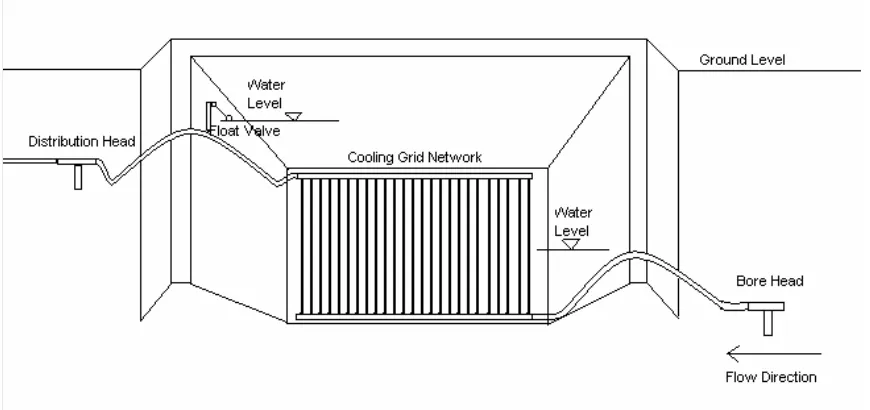
Cooling of the artesian water is achieved by the installation of a cooling grid. A

typical cooling grid is a network of pressurised copper pipes arranged in a radiator

type configuration through which the high temperature bore water is cooled and

delivered to the pipe network distribution head. This grid is submerged in a pond at

a depth of 2 metres where conductive, convective and evaporative cooling effects

dissipate the heat from the artesian water cooling it to below 45 °C before delivery

to the polyethylene pipe system (see Figure 1.1).

(14)

[image:14.595.109.544.133.338.2]

Figure 1.1 Schematic of Typical Cooling Grid

Currently each individual cooling grid is designed and sized using a spreadsheet

design model according to the individual bore temperature and discharge

characteristics to guarantee the required outlet temperature at the maximum

flowrate of the system. The design model utilises a number of variables, constants,

and theoretical calculations to determine the length of pipe that is required for the

desired amount of heat to be transferred from the hot artesian water into the

cooling pond.

This project is aimed at analysing this design model to determine its accuracy in

designing each cooling grid as well as investigating the possible alternative pipe

materials that may be used within each grid to minimise costs whilst maintaining

the desired heat transfer.

The principal aims of this project are to predict and confirm the heat transfer

parameters for cooling grids submerged in water ponds used for cooling artesian

(15)

parameters within the existing design model to more accurately reflect existing

operation.

The specific objectives of the project are as follows:

1. Research material properties of alternate pipe materials, heat transfer

mechanisms through air and water, alternative cooling techniques, flow

characteristics and associated hydraulics theory for pipe networks.

2. Undertake sensitivity analysis of the spreadsheet design model to verify

important variables to aid in pipe material selection.

3. Design a cooling grid test setup for on-site use and an experimental procedure

to compare its performance using differing pipe materials to theoretical

calculations from the existing spreadsheet design, test in field to compare the

heat transfer characteristics in air and water using the selected pipe materials.

4. Comparatively analyse designs tested accounting for costs, material

availability, flow characteristics at different flow rates, cooling performance and

maintenance requirements.

5. Validate and calibrate the current DNR&W design spreadsheet using

measured data, and make recommendations.

6. Write a dissertation and submit by 30/10/2008

By undertaking the necessary research and testing the project will allow increased

accuracy when designing cooling grid systems whilst ensuring the efficient use of

(16)

CHAPTER 2

(17)

Chapter 2: Background Andrew Watt

2.0 Background

2.1 The Great Artesian Basin

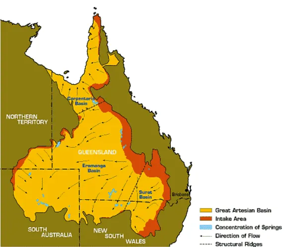
The Great Artesian Basin (GAB) is one of the largest artesian groundwater basins

in the world. It underlies approximately one-fifth of Australia and extends beneath

arid and semi-arid regions of Queensland, New South Wales, South Australia and

the Northern Territory, as shown in Figure 2.1. The GAB covers a total area of over

1 711 000 square kilometres and has an estimated total water storage of 64 900

[image:17.595.183.469.381.629.2]

million megalitres.

(18)

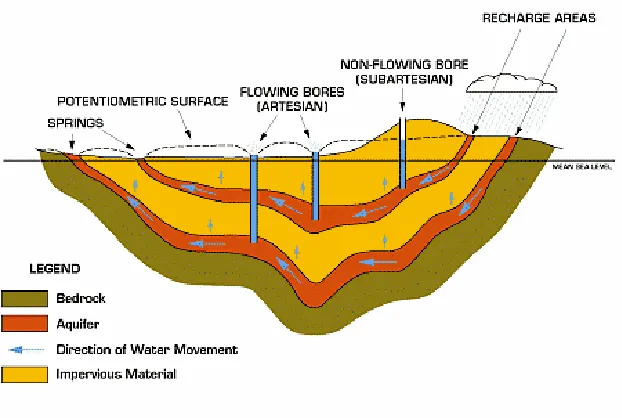
The Great Artesian Basin consists of alternating layers of permeable sandstone

aquifers and impermeable siltstones and mudstones. The depth of these layers

varies from less than 100 metres at the Basin boundaries to over 3 000 metres in

the deeper parts of the Basin. The rate at which water flows through the

sandstones varies between one and five metres per year. Water enters the Basin

by infiltration of rainfall into the outcropping sandstone aquifers mainly along the

western slopes of the Great Dividing Range. This infiltration and flow pressurizes

the water between the permeable and impermeable layers. Pressurised

groundwater is then discharged via approximately 10 000 bores within the Basin

and also naturally from artesian springs in the south-western area because the

[image:18.595.168.479.392.601.2]

potentiometric surface is above ground level (see Figure 2.2).

Figure 2.2: Great Artesian Basin Formation, Source: NR&W Qld.

Water temperatures vary from 30˚C in the shallower areas to up to 99˚C in the

deeper areas. Heating of the water occurs naturally because of its proximity to the

(19)

2.2 Water Usage in the Great Artesian Basin

Prior to human development of the Basin, it is estimated that approximately 300

Megalitres/day of water entered the permeable aquifers of the Great Artesian Basin

in Queensland. All of this inflow, as well as the recharge from other states,

discharged as surface springs, or leakage through the ground surface. In this way

a natural equilibrium of inflow to outflow was maintained.

Europeans first discovered the artesian groundwater of the Great Artesian Basin in

1878 when a shallow bore sunk near Bourke in New South Wales produced

flowing water. A bore is simply a deep hole lined with a metal casing which usually

ranges in diameter from 100 to 300 millimetres. Many bores were soon drilled

throughout the Basin in north-west New South Wales and north-east South

Australia. The first flowing artesian bore in Queensland was drilled in 1887 near

Cunnamulla. Following this discovery, over 500 bores were sunk over the next

decade and by 1915 a total of 1500 bores were supplying an approximate

discharge of 2000 Megalitres/day of uncontrolled artesian water to Queensland

properties.

This seemingly endless supply of water allowed the development of extensive

grazing country throughout the grass plains of western Queensland. Thousands of

kilometres of bore drains were excavated to transport water throughout the

properties. Bore drains are shallow earth trenches which are excavated to allow

the water to travel across the ground surface. However, this increased outflow of

water from the Basin resulted in significant pressure losses with up to a third of all

bores now requiring pumps to bring the water to the surface. Regulations were

introduced to all new bores in 1954, stating that all bores must have a control valve

in place and use pipelines to distribute the water other than open drains. These

(20)

gradual return to equilibrium between recharge and discharge throughout the Basin

today.

2.3 Environmental Impacts

Artesian water, being easy and inexpensive to utilise, is often used inefficiently

after it reaches the surface. In many areas, artesian water is traditionally flowing

uncontrolled from bores into open drains and creeks for stock to drink with nearly

14 000 km of bore drains currently in use throughout Queensland alone. Even in

well-maintained drains, up to 97 per cent of the water is lost through evaporation

and seepage.

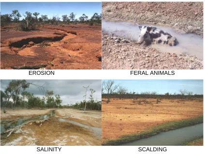
This ineffective and inefficient method of water transport results in serious

environmental impacts and land degradation issues (see Figure 2.3). Some of the

impacts include:

• Feral animals are provided with a habitat and permanent water supply

• Infestations of invasive woody weeds, such as prickly acacia, in and around bore drains

• Erosion problems often result from drains overtopping or breaking their banks

• Salinity problems can be created or aggravated

• Bore drains built across a slope catch run off water, reducing rainfall infiltration below drains and thereby limiting pasture growth

• Concentration of minerals by evaporation (e.g. Sodium and Fluoride) can negatively affect animal health or induce scalding on the soil surface

(21)

EROSION FERAL ANIMALS

[image:21.595.115.539.129.448.2]

SALINITY SCALDING

(22)

2.4 The Great Artesian Basin Sustainability Initiative

The Great Artesian Basin Sustainability Initiative (GABSI) is a joint Federal and

State government project designed for the continued sustainability of the vast

hidden artesian water resource that is the Great Artesian Basin. GABSI’s role is to

work in conjunction with landholders to rehabilitate uncontrolled bores drilled prior

to 1954, and replace bore drains with pipelines delivering the water to tanks and

[image:22.595.159.495.333.585.2]

troughs at designated watering points.

Figure 2.4 Controlled Bore Piped to Tanks, Source: DNR&W

To rehabilitate an uncontrolled bore, the bore and its casing are tested using

geophysical logging probes and a dye test to determine the casing condition, size

and strata details. This information is then used to determine the correct method of

(23)

bore casing near ground level and new headworks, relining of the bore casing by

inserting a smaller diameter pipe into the bore and cementing the annulus between

the two casings, or by plugging the entire bore with concrete to stop flow and

drilling a new bore nearby using inert casing.

Once the bore has been successfully rehabilitated, the water is piped throughout

the areas which the bore drains were previously servicing to new designated

watering points. Each watering point’s location and size is designed to;

• hold at least 2 days supply of water for the stock in the area,

• maintain a maximum walking distance between watering points of 1.5 kilometres for sheep and 2 kilometres for cattle,

• minimise the opportunity for feral animals by using specifically designed high sided troughs and,

• reduce erosion by installing concrete aprons around all watering points.

By capping and piping the artesian bores farm management becomes easier,

productivity increases whilst water is conserved. Other benefits include the

reduction of feral animal habitat, reduced maintenance time, stock weakened by

drought are better able to drink from troughs, the water quality in these piped

systems is considerably better at the watering point when compared to that using

bore drains and when a number of properties are serviced by one bore all

properties, including the ones farthest from the supply are guaranteed water.

A well designed system allows the effective use of the whole property all year

round with pipeline systems that can deliver water to parts of the property that

previously could not be reached by bore drains. Spear traps, which allow animals

to enter safely but not to exit, can be installed at watering points so stock can self

muster and managers can ensure more effective spelling of paddocks as watering

points are turned off. Also, it is possible to deliver food supplements and

(24)

2.5 Cooling Grids

Artesian water can reach very high temperatures because of the naturally high

temperatures at large depths near the earth’s mantle. The temperature of the water

throughout the GAB ranges from 30˚C up to 99˚C at depth. The high temperature

of the water is not of concern when it is flowing uncontrolled into bore drains,

however when the water is piped the temperature presents a problem in terms of

polyethylene pipe degradation.

The medium density polyethylene (PE 80B) pipe that is used for piping the artesian

water throughout the GAB requires a temperature below 45°C to maintain a design

lifespan of greater than 50 years (James Hardie Pipelines, 1997). At higher

temperatures the PE 80B pipe will only remain viable for 25 years or less because

of the heat deterioration of the pipeline. Hence, the water must be cooled before

entering the reticulation system.

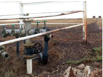
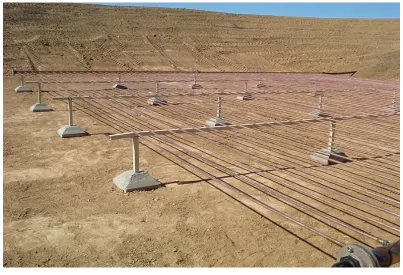
The current practice used to cool artesian water utilises the natural pressure of the

bore to pump the hot water through a network of 19.1mm plain walled copper pipes

submerged in an earthen walled pond at a depth of 2 metres (see Figure 2.5). The

copper pipes are arranged in parallel which are fed and collected by 100 mm

copper manifolds at either end (see Figure 2.6). Each copper grid is sized

according to the individual bore characteristics of pressure, temperature, and

maximum flowrate using a spreadsheet model which will be discussed later.

At present, the cooling grid design model spreadsheet that is used to size each

grid in each scheme is relatively untested. There is a need to validate this design

model to ensure the correct sizing of grids for sustainable resource management

and to ensure that the theoretical calculations are truly representative of in field

results. This study will focus on the theoretical versus practical performance of the

(25)

[image:25.595.118.533.128.387.2]

Figure 2.5 Installed Cooling Grid, Source: DNR&W

[image:25.595.124.527.451.726.2]

(26)

CHAPTER 3

(27)

Chapter 3: Literature Review Andrew Watt

3.0 Literature Review

This chapter will review literature on previous work to expand upon the material

outlined in previous sections whilst providing a context for this project. A review of

the physical heat transfer principles and alternative cooling practices will follow to

provide an increased understanding of the subject.

3.1 Review of Previous Work

Copper cooling grids are a relatively new cooling method for artesian water and

have only been in use for less than a decade. Water running uncontrolled into

drains required no cooling as it was exposed to convective and evaporative cooling

effects. Prior to the use of copper grids piped artesian water was cooled using steel

or polyethylene pipe submerged in an earthen walled dam. This system utilised

little to no design process. The steel or polyethylene would simply be replaced as

necessary. Some piped schemes employed no cooling technique at all which

rapidly deteriorated the polyethylene pipe requiring regular maintenance.

Since the copper cooling grids have been utilised by the Department of Natural

Resources and Water many changes to their design have occurred. It was thought

by the GABSI staff that by using copper pipe with a ‘crinkled’ or ‘finned’ surface the

heat transfer into the pond would be greater because of the increased surface area

of the pipe. Over time this practice was deemed unreliable as the finned pipe

allowed for considerable algal growth requiring frequent cleaning to maintain the

desired heat transfer capacity. This algal growth was factored into the design for a

(28)

performance and loss of heat transfer. The choice of pipe was converted back to

plain walled copper pipes in both the design and installation of systems.

The design model used in the creation of copper cooling grids has also been

subject to change over time and has come under review in previous studies. As the

model has developed and been added to over time, a broader scope of

calculations has been included allowing for increased accuracy in design.

It is important to note the above continued changes to cooling grids and their

design to understand the previous studies undertaken and set the context in which

they were produced.

Martin (2003) analysed the practical versus theoretical performance of finned

copper cooling grids and developed a design spreadsheet to account for any

inaccuracies. Martin (2003) tested the theory on two separate bores using varied

flowrates over a period of time. The flow control valve used in their experiments

significantly affected the pressure in the system inducing a 2 to 3 metre head loss

through the valve. In addition to the experiments performed, Martin (2003) also

evaluated the possibility of modifying current practice by employing different

materials. No practical or theoretical testing was conducted and only cooling

towers and stainless steel as an alternative pipe material in the grid were

mentioned.

Martin (2003) states that…

“stainless steel does not offer the heat transfer capabilities of copper so

a larger grid is required…the anaerobic environment in a cooling pond

would not allow the protective oxide film to develop and therefore you

would not expect stainless steel to stand up to corrosion better than

(29)

These claims were examined during this project’s research and testing.

Martin (2003) reports that cooling towers offer no substantial benefit to the cooling

of piped artesian water in Queensland because of the loss of natural bore pressure

and requirement of power for pumping. Martin (2003) confirmed Eigland (2000)

which is a report for the ‘Capping and Piping the Bore Program’ in New South

Wales by the Department of Land and Water Conservation. The schemes are

designed in Queensland to utilise the natural bore pressure and flow so as to

remove the power requirement for pumping.

Webb (2002) evaluated the performance of the addition of heat dissipating fins to

the cooling grid pipes as well as varied pipe wall thicknesses. These heat

dissipating fins were proven to be impractical during installation. Webb (2002) also

analysed the performance of the grids without any cost evaluation giving no real

world validation of the ‘improved’ design. The fins also promoted increased

external algal growth inhibiting the overall heat transfer and introducing the

requirement of manual cleaning of the pipe exteriors.

An internal report conducted by Alsemgeest and Zuino (2002) for the Department

of Natural Resources and Water evaluated the necessity of cooling grids

altogether. The report investigated the effects of piping the water claiming the

increased pressure from piping would reduce the bore temperature enough to

allow for a sacrificial length of polyethylene pipe to be used close to the bore to

provide an area for cooling. The difficulty in prediction of the length of sacrificial

pipe required presented a problem as well as the prediction of temperature

decrease from pressure recovery. PEX polyethylene pipe is a new pipe designed

to withstand temperatures up to 80°C. This PEX pipe may become a viable option

for an extended length from the bore head to allow for cooling as its price

decreases with continued usage. This pipe is currently in use by GABSI to connect

(30)

connection distance. The result of the Alsemgeest and Zuino (2002) report

certainly presents an area of further study when the price of PEX pipe reduces.

Watt (2007) analysed the theoretical performance of varied cooling grid pipe sizes

and grid configurations. The report used the current design model to investigate

the performance of cooling grids with larger and smaller pipes as well as having a

‘stacked’ grid with one set of pipes above another. Cost, performance,

maintenance requirements and ease of installation were considered as criteria for

optimisation which yielded a recommendation of a 31.8mm pipe size for the current

grid and a 38.1mm pipe size for a ‘stacked’ design. Although real world costs were

involved no practical testing was conducted which assumed the design model

reflected actual performance. Watt (2007) indicated the necessity of cooling grid

performance evaluation to optimise design.

It is still unknown whether the current design model accurately represents in situ

results which are the main focus of this project. As a result of previous

investigations there is a need to validate the design model to analyse how the

previous findings have been used to alter the current model. At this point in time,

NR&W do not have confidence that the existing cooling grid design model

(31)

3.2 Heat Transfer Mechanisms

Heat transfer is defined as the energy transferred when a temperature gradient

exists within a system, or whenever two systems at different temperatures are

brought into contact (Kreith & Bohn, 2001). The physics of heat and heat transfer

are well known but are included here in a brief review on the subject.

There are three main modes of heat transfer. They are conduction, convection and

radiation. Each of these will be discussed in-turn.

3.2.1 Conduction

Conduction of heat occurs in gases, liquids and solids and is assumed to involve

no bulk motion. Heat is transferred from rapidly moving high energy molecules

which randomly collide with low energy slow moving molecules in a fluid where a

temperature gradient exists (Janna, 2000). These random collisions exchange

momentum and energy and therefore heat. It is possible to quantify the amount of

heat transferred per unit of time through the mode of conduction using Fourier’s

Law of Heat Conduction, equation 3.11 (Incropera & DeWitt, 1996).

L T k q L T T k q ∆ = ⇒ − −

= 1 2

(3.11)

where q = heat flux perpendicular to direction of transfer [ W/m2 ];

k = thermal conductivity [W/m.K ];

L = length [ m ]; and

(32)

3.2.2 Convection

Convection of heat through liquids is comprised of two mechanisms. Heat is

transferred by random molecule collisions as outlined above as well as by the bulk

motion within the fluid (Incropera & DeWitt, 1996). Heat transfer by convection can

be forced or natural, or free, in nature. Forced convection occurs when an external

force such as an agitator or pump creates the fluid motion which will transfer heat

between areas of higher temperature and lower temperature. In contrast, natural or

free convection occurs from the buoyancy forces which are created by the density

differences between areas of higher temperature and lower temperature (Kreith &

Bohn, 2001).

In both forced and free convection the heat flux created can be quantified using

Newton’s Law of Cooling, equation 3.12 (Incropera & DeWitt, 1996).

(

T1 T2

)

h

q= − (3.12)

.

where q = heat flux perpendicular to the direction of transfer [ W/m2 ];

h = convection heat transfer coefficient [W/m2.K ]; and T = temperature [ °K ].

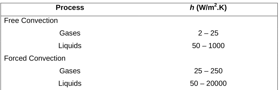
This law utilises a proportionality constant, h [ W/m2 .K ], known as the convection

(33)

[image:33.595.104.548.168.312.2]

Table 3.1 Typical values of the convection heat transfer coefficient

(Incropera & DeWitt, 1996).

Process h (W/m2.K)

Free Convection

Gases 2 – 25

Liquids 50 – 1000

Forced Convection

Gases 25 – 250

Liquids 50 – 20000

It is also important to note that if a temperature gradient exists between a fixed

surface and a free fluid a consequence is the development of a region in the free

fluid where the bulk velocity varies from zero at the surface to a finite value

associated with the relative conditions. This is because of the viscous forces within

the fluid and is referred to as thermal boundary layer development which will vary

from system to system (Kreith & Bohn, 2001).

3.2.3 Radiation

Radiation or thermal radiation is the energy emitted by a body by virtue of its

temperature and at the expense of its internal energy. Radiation needs no

transport medium and is most efficient in a vacuum (Incropera & DeWitt, 1996). All

heated solids, liquids and some gases emit thermal radiation to their surroundings.

This heat flux can be quantified using equation 3.13 if both the surroundings and

(34)

(

)

(

)

(

2

)

2 2 1 2 1 2 1 T T T T h where T T Ah q + + = ⇒ − = εσ (3.13)

where q = heat flux perpendicular to the direction of transfer [ W ]; h = radiation heat transfer coefficient [W/m2.K ];

A = surface area [ m2 ];

ε_{= emissivity [ dimensionless ];}

σ_{= Stefan-Boltzmann constant [ 5.67 x 10}-8_W/m2_.K4_];

T1 = surface temperature [ °K ]; and

T2 = surrounding temperature [ °K ];

3.2.4 Heat Transfer in Cooling Grids

All three heat transfer mechanisms contribute to heat loss through cooling grids.

Heat energy is conducted through the metal pipes into the pond. Free convection

occurs within the pond as the temperature difference between the pipes and the

pond creates a buoyancy effect from density changes resulting in convection

currents throughout the pond. Heat is also radiated from the hot bore water through

the pipe and into the pond.

Solar radiation is of great importance as well because of its contribution to heat

loss. As solar radiation strikes the surface of the cooling pond it contributes to the

evaporation of water molecules. This evaporation requires a large input of energy

from the molecule’s surroundings as it changes phase from liquid to gas. This

energy comes partly from solar radiation but mainly from the surrounding water

molecules, hence cooling the water in the pond. This is known as the evaporative

cooling effect (Allen et al, 1998). Ambient temperature and windspeed are also

(35)

Cooling grids are designed to provide the appropriate amount of heat transfer for

the system’s maximum designed flowrate, which occurs as the pipeline system is

filled. After the initial ‘filling’ of the pipe, tank and trough system the actual

operating flowrate is considerably reduced. The flowrate required to maintain this

level is dependent upon the stock drinking requirements, losses due to pipe

leakage and evaporation from the troughs. This means that over 99% of the

system’s working life will be at a flowrate considerably less than that required at fill.

3.3 Cooling Grid Design Spreadsheet

A Microsoft Office Excel spreadsheet has been developed by NR&W using worked

examples from the POLIPLEX Polyethylene Pipe Design Textbook, 1997 from

James Hardie Plumbing and Pipelines Pty Ltd, Australia. The spreadsheet is used

to calculate the length of pipe required in the grid to reduce the temperature of the

water in the pipe to the required outlet temperature of below 45 °C, the number of

pipes required in the grid using a predetermined individual pipe length as well as

the friction loss through the grid.

The user inputs are of peak flow rate, inlet temperature, pressure head at inlet and

the length of individual pipe between the manifolds. The spreadsheet model will be

(36)

3.4 Alternative Water Cooling Practices

There are many ways in which water can be cooled. However the method chosen

is dependent upon the individual cooling purpose, cost, infrastructure, power

availability and design efficiency to name a few. Some commonly used water

cooling practices include gas refrigeration, cooling tanks/towers, passive radiator

cooling systems and heat pipes. These alternative water cooling techniques to

cooling grids will be discussed to outline any possible applications to the GABSI

schemes.

3.4.1 Gas Refrigeration

Gas refrigeration involves a process which utilises the heat changes as a

substance is evaporated and condensed continuously throughout a system of

(37)

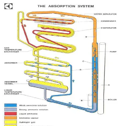
[image:37.595.132.512.131.537.2]

Figure 3.1 Gas Absorption System. Source: Lehman’s Gas Refrigerators, 2007

This continuous absorption system has no moving parts, absorbs heat efficiently

and requires minimal maintenance. However, a supply of heat either from

electricity, gas or kerosene is required to drive the system. Put simply, liquid

ammonia is passed through a network of tubes called the evaporator, the ammonia

then vaporises because of a change in pressure caused by the introduction of

(38)

gas is then mixed with water to separate it from the surrounding hydrogen and then

boiled to extract the pure ammonia gas. This gas is then condensed in a heat

exchanger to form liquid ammonia and the process begins again (Lehman’s Gas

Refrigerators, 2007).

3.4.2 Cooling Tanks/Towers

Cooling towers are used in the many industries to dissipate waste heat to the

atmosphere through the cooling of a water stream to a lower temperature. This

cooling technique employs the evaporative cooling effect where a small amount of

the water is allowed to evaporate to provide cooling to the rest of the water stream

(Cooling Technology Institute, 2007). The heat energy from the water stream is

transferred to the surrounding air increasing its temperature and relative humidity.

This heated air is then released to the atmosphere and replaced with cooler

ambient air through inlets at the base of the tower using the forces of convection.

Cooling tanks are simply water holding tanks which give the heated water time to

cool. These tanks also utilise the evaporative cooling effect to remove the majority

of the heat energy to the atmosphere. Cooling tanks can be situated on the ground

surface or raised off the ground to take advantage of gravitational forces for cool

water delivery.

3.4.3 Passive Radiator Cooling Systems

Another cooling technique which utilises the convection mode of heat transfer is

(39)

similar to that used in car radiators. These fins are filled with the water to be cooled

and subjected to free and forced heat convection in a natural outdoor environment.

The heat is transferred through the fins through the mode of conduction and

removed to the atmosphere by the mode of convection. To maintain optimum

conditions passive radiator cooling systems should be shaded from sunlight to

maintain the maximum possible temperature gradient between the heated water

and the atmosphere and prevent solar radiation interference.

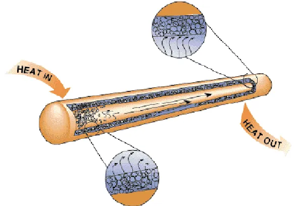
3.4.4 Heat Pipes

A heat pipe is simply a pipe that can quickly and efficiently transport heat from one

area to another. They are often referred to as superconductors of heat because of

their extraordinary heat transfer capabilities (CheResources, 2008). Heat pipes

consist of a sealed copper or aluminium tube. Within this tube the inner surface is

lined with a wick-like structure which allows for the transportation of a liquid or

working fluid. The working fluid is usually liquid ammonia which evaporates from

the wick when subjected to heat and travels through the hollow centre of the tube

in gaseous form. If the heat pipe is subjected to a hot and cool environment on

either end, the ammonia gas will then condense at the cool end and be absorbed

back into the wick. The ammonia liquid then travels back to the hot end through the

wick due to gravitational forces, if the pipe has a vertical orientation as well as by

the flux created by the evaporating ammonia at the other end (Chisholm, 1971). A

(40)

[image:40.595.181.472.134.338.2]

Figure 3.2 Heat Pipe Source: CheResources, 2008

Heat pipes are used in a wide range of cooling applications including laptops,

refrigeration, air-conditioning, heat exchangers and in space technology.

3.4.5 Applications to Artesian Bore Water Cooling

Gas refrigeration is a minimal maintenance self sufficient system which requires

only one input of heat. It presents as a possible alternative for some artesian bore

water cooling systems if the heat of the bore could be used as this heat source.

The temperature of the bore would need to be higher than that of the boiling point

of the hydrous ammonia. The relative size is a limiting factor and the system’s

ability to handle high flowrates may present as a problem which would require

significant development if this process was chosen as an alternative.

Cooling towers require the use of some of the water stream for cooling. Artesian

(41)

pressure of the bore to remove the need for powered pumping, therefore cooling

towers may not be a viable option for this type of water cooling. Cooling tanks

however, are able to utilise gravity for the system’s pressure requirements. This

may prove effective in the Queensland artesian bore piping schemes where the

terrain is mostly flat and the bore pressure is sufficient to reach an elevated tank.

Cooling tanks are used in conjunction with powered pumps in most New South

Wales piping schemes.

Passive radiator cooling systems can maintain the bore pressure, are relatively

cheap and open up the possibility of recycling used radiators. However, as air has

a low heat transfer capacity a larger surface area for cooling would be required.

Increased development of this passive cooling technique may increase its potential

for its application in artesian water cooling systems.

Heat pipes, although relatively more expensive than other cooling techniques,

require little to no maintenance, are fully self sufficient and depend on the physics

of the working fluid. Applications of this technology to the cooling of artesian bore

water would require significant research and design to extract the heat energy from

the water and dissipate it to the environment whilst maintaining the natural

pressure of the bore.

The above systems all require fewer earthworks than the current cooling grid

system which would reduce costs and maintenance requirements. Further

investigation into one or all of these systems may be viable in the future but was

(42)

3.5 Flow Characteristics in Pipelines

As the velocity of fluid flowing within pipelines change, the physical characteristics

of the flow profile also vary. At smaller velocities water particles flowing in pipelines

are observed to move in straight lines which slide over one another with little to no

mixing occurring within the fluid. The fluid appears to move by the sliding of

laminations of miniscule thickness over adjacent layers (Finnemore & Franzini,

2002). Hence, this type of flow is labelled laminar flow.

As the velocity within a pipeline increases, the paths of the water molecules

become more varied. A period of transition is observed in which the water particle

movement may become wavy with no definite wave frequency and with a small

amount of particle mixing. Following this transition period turbulent flow is

observed. Turbulent flow is characterised by the irregular motion of a large number

of water particles with no observable pattern during a small time interval

(Finnemore & Franzini, 2002).

The type of fluid flow can be easily determined when the flow parameters are

known using Reynold’s number. Reynold’s number is simply a ratio of inertia forces

to viscous forces and assumes no gravitational or capillary action in a completely

filled pipeline (Finnemore & Franzini, 2002). Reynold’s number values of between

0 and 2000 are identified as laminar flows, values of between 2000 and 4000

identify the transition period of flows and values of above 4000 are categorised as

turbulent flows. Reynolds number can be calculated using equation 3.5 (Finnemore

(43)

ν

VD

R_e= (3.5)

where Re = Reynold’s number [ dimensionless ];

V = flow velocity [ m/s ];

D = pipe diameter [ m ]; and

ν_{= kinematic viscosity of fluid [ m}2_{/s ].}

3.6 Pipe Material Selection

In order to identify improvement in the cooling grid design differing pipe materials

need to be analysed to ensure continuity in the model as well as to optimise the

overall design. Pipe material selection is important because of availability, cost,

maintenance requirements, application suitability, heat transfer parameters and

ease of installation.

To maintain good experimental design copper was chosen as the control material.

Copper is the pipe material of choice at present and the design model was created

for this metal. Copper has been used in the design of cooling grids because of it’s

availability in the correct diameter, excellent heat transfer abilities and resistance to

corrosion (Janna, 2000).

Aluminium was the second choice for pipe material. Aluminium is similar to copper

in that it is low cost, offers good heat transfer capacity, good workability and

resistance to corrosion with the formation of an aluminium oxide film to resist

oxidation (Janna, 2000). The third choice for pipe material was stainless steel.

Stainless steel was chosen to provide a comparison in heat transfer capacity

(44)

Stainless steel is also relatively low cost and has good availability in the correct

diameter. A chromium oxide film is present on stainless steel when exposed to

oxygen which provides rust protection (Janna, 2000). Martin (2003) also

discounted stainless steel as a possible alternative, as outlined in Section 3.1, so

[image:44.595.111.541.290.439.2]

the material is included here to prove or disprove Martin (2003).

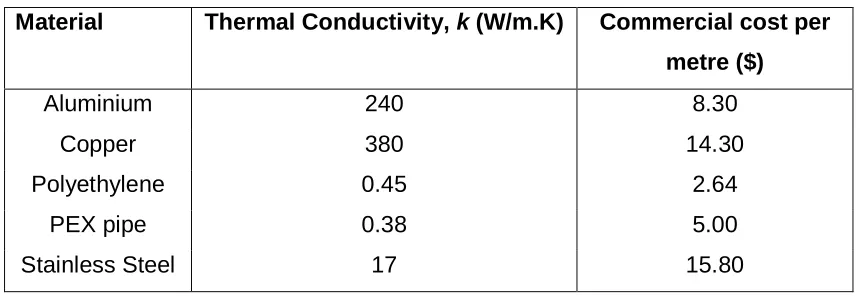
Table 3.5 Thermal conductivity of some materials. Source: Janna, 2000

Material Thermal Conductivity, k (W/m.K) Commercial cost per

metre ($)

Aluminium 240 8.30

Copper 380 14.30

Polyethylene 0.45 2.64

PEX pipe 0.38 5.00

Stainless Steel 17 15.80

The spreadsheet model will now be discussed in detail to provide an understanding

of the model itself, the sub-models and hydraulic equations used. A sensitivity

analysis of the model will be discussed to identify important variables and areas for

(45)

CHAPTER 4

MODEL DESCRIPTION & SENSITIVITY

(46)

Chapter 4: Model Description & Sensitivity Analysis Andrew Watt

4.0 Model Description and Sensitivity Analysis

The spreadsheet model developed by Andrew Brier for NR&W utilises worked

examples from the POLIPLEX Polyethylene Pipe Design Textbook, 1997 from

James Hardie Plumbing and Pipelines Pty Ltd, Australia to determine the correct

cooling grid size for each individual GABSI scheme.

User inputs and defined constants are used to calculate the convection heat

transfer coefficients for forced convection in the cooling grid pipes and natural

convection in the cooling pond. These heat transfer coefficients are then used to

calculate the overall heat transfer coefficient for the entire system. The amount of

heat required to be transferred to the pond can then be determined.

Temperature gradients, pipe radii and material properties are then used to

calculate the area of pipe material, and therefore the pipe length, required to

transport this heat. The frictional head loss through the grid is also calculated.

4.1 Model Calculations

The model is complex and interactive with values taken from graphs and trials

being calculated to determine the correct grid size. The user inputs, defined

constants and equations 4.1 to 4.25 are outlined below to illustrate the processes

(47)

4.1.1 User Inputs

Peak Water Demand (L/s) - Q

Inlet / Bore Temperature (°C) - Ti

Pressure Head at Inlet (m head) - P

Length of Individual Pipe (m) - L2

Required Outlet Temperature (°C) - To

Water Temperature of Pond (°C) - Tp

Inside Diameter of Pipe (m) - Di

Outside Diameter of Pipe (m) - Do

4.1.2 Defined Constants

Specific Heat of Water

Cw = 4180 J / kg .°C

Conduction Coefficient for Pipe Material

Kc = 380 W / m . °C

Conduction Coefficient for Water

Kw = 0.56 W / m . °C

Density of Water

(48)

Kinematic Viscosity of Water (calculated from graph)

ν = 0.000000500 m2 / s

Fouling Factor for Water (>50˚C)

Rf = 0.0 m2 . °C / W

Coefficient of Roughness

k = 0.000003 m

Pi

π = 3.14159… dimensionless

4.1.3 Calculations

Average Temperature in Grid – Ta (°C)

2 ) (Ti To

Ta= + (4.1)

Inside Radius of Pipe – ri (m)

2

i i

D

(49)

Outside Radius of Pipe – ro (m)

2

o o

D

r = (4.3)

Left Fluid Temperature Difference – ∆Ta (°C)

Tp Ti

Ta= −

∆ (4.4)

Right Fluid Temperature Difference – ∆Tb (°C)

Tp To

Tb= −

∆ (4.5)

Log – Mean Temperature Difference – ∆TLM (°C)

) / ln( Tb Ta

Ta Tb TLM ∆ ∆ ∆ − ∆ = ∆ (4.6)

Correction Factor – F (dimensionless)

Calculated from graph

Mean Temperature Difference – ∆TMEAN (°C)

F T TMEAN =∆ LH *

∆ (4.7)

Velocity in Pipes – V (m / s)

n Di Q V      

= ( *( )/4)

(50)

Reynold’s Number in Pipes – Re (dimensionless)

ν

) * (

Re= Di V (4.9)

Prandtl Number in Pipes – Pr (dimensionless)

Kw Cw* * ) (

Pr= ρ ν (4.10)

Nusselt Number in Pipes – Nu (dimensionless)

4 . 0 8 . 0 Pr * Re * 023 . 0 = Nu (4.11)

Heat Transfer Coefficient in Flowing Water – h1 (W / m2 . °C)

Di Kw Nu

h1 =( * ) (4.12)

Mean Temperature for Natural Convection in Pond – Tm (°C)

2 ) (Ta Tp

Tm= + (4.13)

Kinematic Viscosity for Natural Convection – ν (m2 / s)

(51)

Volume coefficient of Expansion for Water – B (m3 / °C)

Calculated from graph and Tm

Grashof Number – Gr (dimensionless)

2 3 ) * ) ( * * ( ν

β Ta Tp Do g

Gr= − (4.14)

Rayfield Number – Ra (dimensionless)

Pr *

Gr

Ra= (4.15)

C (dimensionless) Calculated from graph and Ra

n (dimensionless) Calculated from graph and Ra

Nusselt Number for Natural Convection in Pond – Nu1 (dimensionless)

n Ra C

Nu₁ = * (4.16)

Heat Transfer Coefficient in Still Water – hs (W / m2 . °C)

Do Kw Nu hs ) * ( 1 = (4.17)

Modified Coefficient for Algal Growth – h2 (W / m2 . °C)

s h

(52)

Heat required to be transferred to pond – q (W)

) (

* *

*Cw Ti To

Q

q= ρ − (4.19)

Overall Heat Transfer Coefficient – U (W / m2 . °C)

            + + + + = ) * ( ) * ) ( ) ln( * ) ( ) 1 ( 1 2

1 r h

r Rf r r r r Kc r Rf h U o i o i i o i (4.20)

Area of Pipe Required – A (m2)

) *

(U TMEAN q A

∆

= (4.21)

Total Length of Pipe Required – L (m)

) * ( Di A L π

= (4.22)

Pipe Friction Factor – f (dimensionless)

            + +

= 0.33

Re 106 ) * 20000 ( 1 0055 . 0 Di k f (4.23)

Frictional Loss through Pipes – hf (m head)

      +       = 100 20 1 * ) * * 2 ( ) * *

( ₂ 2

Di g L f

(53)

Remaining Head at Outlet – Pt (m head)

hf P

Pt= − (4.25)

The model produces outputs of total length of pipe required, friction loss through

the grid, number of pipes required and the length of each pipe. The length of each

pipe is a user defined input and is reported here as a reminder to the user. The

number of pipes required is simply the total length divided by the length of each

pipe.

Each 6 metre cooling grid manifold has 30 pipe outlets, and the cooling pipes are

also produced in 6 metre lengths. Knowing this, the user can then use the model to

vary the length of each pipe, in multiples of 6 metres, to gain an output from the

model of the number of pipes required to as close to a multiple of 30 as possible.

The user can then design the appropriate sized cooling grid using these values.

For example, with the individual pipe length defined by the user as 18.0 metres, the

model declares that 77 pipes of this length is required to transfer the calculated

amount of heat in a hypothetical cooling grid system. Therefore, the cooling grid

would need to be 18.0 metres long by 3 manifolds, or 18.0 metres, wide. This

would include 13 extra pipes and would therefore be over designed.

By varying the length of each pipe to 24.0 metres, the model then declares that

only 55 pipes are required for cooling and the system would now be 24.0 metres

long by 2 manifolds, or 12 metres, wide. Only 5 extra pipes would be required,

(54)

4.2 Sensitivity Analysis

A sensitivity analysis of the spreadsheet design model was conducted at the

beginning of the project to identify important variables. By identifying the most

influential components of the design, the testing and experimentation phases were

better able to focus on analysing these areas. Each input and some constants

were varied by a percentage and the relative change in the model’s output was

noted. The percentage by which each input was varied depended upon their initial

values and their purpose in the design. For example, the temperature of the pond

could not be varied by 50% as it may become higher than the bore inlet

temperature which is highly unlikely in a real world situation. Table 4.1 below

[image:54.595.105.554.436.738.2]

outlines the results of the sensitivity analysis.

Table 4.1 Sensitivity Analysis Results

Variable Material Model Output (No. of pipes) Variance

Copper k = 380 52 0 %

Aluminium k = 240 52 0 %

Thermal Conductivity k

(W/m.K)

Stainless Steel k = 17 54 3.8 %

Variable % Varied Initial Value Output (No. of pipes) Variance

+ 50 % 78 + 50 %

Maximum Flowrate Q

(L/s) _{- 50 %}

52

26 - 50 %

+ 10 % 68 + 33 %

Bore Temperature Ti

(°C) _{- 10 %}

52

33 - 33 %

+ 50 % 52 0 %

Pressure head at Inlet P

(m) _{- 50 %}

52

52 0 %

+ 10 % 27 - 48 %

Outlet Temperature

Required To (°C) _{- 10 %}

52

90 + 73 %

+ 10 % 71 + 37 %

Pond Temperature Tp

(°C)

- 10 %

52

(55)

From the sensitivity analysis, the most important variables were identified as

maximum flowrate as well as the outlet, bore and pond temperatures. The required

outlet temperature proved to be the most influential factor with larger variances in

the model output than the other input variables. For design purposes it is important

to note that this required outlet temperature remains constant. Maximum flowrate,

Q, affected the model output by the same value as it was varied. The bore, Ti, and

pond, Tp, temperatures altered the model output by slightly greater than that by

which the variables were altered. Pressure head at inlet had no effect on the model

output which was expected as this value is used in pressure and friction

calculations only.

Interestingly, the thermal conductivity, k, of the pipe material had no significant

impact on the model output. This was quite surprising as indicated by the change

from copper to stainless steel values of more than 2200% yielding a variation in

model output of only 3.8%.

The results of the sensitivity analysis provided an overall perspective of the

model’s ability to cope with change and allowed for the selection of alternative pipe

materials to be unrestricted by their relative thermal conductivity values. The

sensitivity of the other various inputs will allow for a more guided model analysis

and optimisation.

The following chapter outlines the field testing procedure, justification and

(56)

CHAPTER 5

(57)

Chapter 5: Experimental Methodology Andrew Watt

5.0 Experimental Methodology

5.1 Field Testing Procedure

Testing of alternative cooling grid pipe materials was conducted on the ‘Beverleigh’

property bore, 5 kilometres east of Dirranbandi, Qld. The bore itself has a

maximum temperature of 62°C and maximum discharge o f approximately 15 L/s.

The headworks of the bore have been recently rehabilitated by NR&W staff and the

property was in the process of becoming fully serviced by pipelines to tanks and

troughs. A 16m by 16m cooling pond and 12m by 12m grid was installed

approximately 30 metres north east of the bore head. The cooling grid had not yet

been in service because of a damaged coupling to a manifold.

The three pipe materials to be tested were aluminium (28.4mm outer diameter

(OD)), copper (19.1mm OD), and stainless steel (25.4mm OD). The testing

apparatus was set up on the western edge of the cooling grid within the dry pond

with steel posts and hooks to hold the single 12m pipe material approximately 0.5m

above the pond floor (see Figure 5.1). The water inlet and outlet temperatures

were recorded using an EMS 050D data logger equipped with RTD PT100

temperature probes. The probes were inserted into the centre of the flow using a

blanking plug in an upright poly T-junction and were sealed using rubber

grommets. The data logger recorded readings at 15 second intervals.

Discharges representing 1, 3, 5 and 7 L/s through an entire grid were simulated in

the single pipe using 0.017, 0.05, 0.083 and 0.117 L/s flowrates respectively. This

was calculated by dividing the flow by the number of pipes within the grid, in this

(58)

Chapter 5: Experimental Methodology Andrew Watt

overall operating spectrum of cooling grid systems as well their particular flow

characteristics. The velocity profile and Reynolds number of the 1 and 3 L/s

flowrates indicates laminar and transitional flow respectively, whereas the 5 and 7

L/s flowrates represented the turbulent end of the spectrum. Kinematic viscosity, ν_,

[image:58.595.112.542.292.540.2]

was varied to 5.0 x 10-6 m2/s for water at 60 °C.