Applications of sensitivity analysis for probit stochastic network equilibrium

This is a repository copy of Applications of sensitivity analysis for probit stochastic network

equilibrium.

White Rose Research Online URL for this paper:

http://eprints.whiterose.ac.uk/2556/

Article:

Clark, S.D. and Watling, D.P. (2006) Applications of sensitivity analysis for probit stochastic

network equilibrium. European Journal of Operational Research, 175 (2). pp. 894-911.

ISSN 0377-2217

https://doi.org/10.1016/j.ejor.2005.06.012

[email protected] https://eprints.whiterose.ac.uk/ Reuse

See Attached Takedown

If you consider content in White Rose Research Online to be in breach of UK law, please notify us by

White Rose Research Online

http://eprints.whiterose.ac.uk/

Institute of Transport Studies

University of Leeds

This is an author produced version of an article published in European Journal of

Operational Research. It has been peer reviewed but does not contain the

publishers formatting or pagination.

White Rose Repository URL for this paper:

http://eprints.whiterose.ac.uk/

2556/

Published paper

Clark, S.D.; Watling, D.P. (2006)

Applications of Sensitivity Analysis for Probit

Stochastic Network Equilibrium.

European Journal of Operational Research,

(175), pp.894-911.

APPLICATIONS OF SENSITIVITY ANALYSIS FOR

PROBIT STOCHASTIC NETWORK EQUILIBRIUM

Stephen D. Clark

1

& David P. Watling*

Institute for Transport Studies, University of Leeds, UK

*Corresponding Author:

David P. Watling

Institute for Transport Studies University of Leeds,

Leeds LS2 9JT, U.K. Tel: +44 113 343 6612 Fax: +44 113 343 5334

Email: [email protected]

Date: May 25th 2005

1

Abstract - Network equilibrium models are widely used by traffic practitioners to aid them in

making decisions concerning the operation and management of traffic networks. The common

practice is to test a prescribed range of hypothetical changes or policy measures through

adjustments to the input data, namely the trip demands, the arc performance (travel time)

functions, and policy variables such as tolls or signal timings. Relatively little use is, however,

made of the full implicit relationship between model inputs and outputs inherent in these

models. By exploiting the representation of such models as an equivalent optimisation

problem, classical results on the sensitivity analysis of non-linear programs may be applied, to

produce linear relationships between input data perturbations and model outputs. We

specifically focus on recent results relating to the probit Stochastic User Equilibrium (PSUE)

model, which has the advantage of greater behavioural realism and flexibility relative to the

conventional Wardrop user equilibrium and logit SUE models. The paper goes on to explore

four applications of these sensitivity expressions in gaining insight into the operation of road

traffic networks. These applications are namely: identification of sensitive, ‘critical’

parameters; computation of approximate, re-equilibrated solutions following a change

(post-optimisation); robustness analysis of model forecasts to input data errors, in the form of

confidence interval estimation; and the solution of problems of the bi-level, optimal network

design variety. Finally, numerical experiments applying these methods are reported.

Keywords: Traffic, equilibrium network flows, robustness and sensitivity analysis, probit

1. INTRODUCTION

The Deterministic User Equilibrium (DUE) is a multi-commodity network flow problem

commonly found in road transport which arises from a supposed ‘game’ between the

road-users in the style of a Nash equilibrium (Nash, 1951). In the DUE problem, a vector of

network arc flows must be determined which is consistent with individual drivers selecting

paths so as to minimise their own generalised travel times (a weighted combination of factors,

in travel time equivalent units), where the arc travel times depend on the arc flows (Beckmann

et al, 1956). Such models are used widely in practice to plan transport facilities for urban

areas, in particular policies that may affect the demand for travel (in terms of the given trip

rates between origin and destination nodes), the supply of road network capacity (impacting

on the arc relationships between travel time and flow), or the non-time attributes, such as

tolls, that impact directly on drivers’ generalised travel times. The reader is referred to

Nguyen et al (1996), for example, for a survey of the literature on the theory and application

of such models.

Despite the optimization being at the individual driver, non-cooperative level, rather than a

system optimization, it has long been known that a modified system-level, convex

optimization problem exists which recovers the DUE solution, at least for ‘separable’

problems where an arc’s travel time is independent of flows on other arcs (Beckmann et al,

1956), allowing efficient solution methods for convex problems to be applied (e.g. Frank &

Wolfe, 1956). Many variants on this basic DUE model exist, with specialist solution

techniques, such as problems with link interactions (e.g. Nguyen & Dupuis, 1984; Patriksson

& Rockafellar, 2003), non-additive generalised path travel times (e.g. Chen et al, 2001b), and

DUE incorporating intra-period dynamic phenomena (e.g. Wie, 1995; Chen et al, 2001a)

In practice, determining all the factors impacting on generalised travel times is no trivial task,

and in any case the perceptions of these vary across individuals and between trips. An

in which unobserved, uncertain or heterogeneous elements of the generalized travel times are

reflected through randomly distributed additive components. Drivers select paths based on

perceived generalized travel times ⎯ the sum of the deterministic part and random

disturbance ⎯ based on behavioural random utility theory (Sheffi, 1985). Within the SUE

family many specific model forms may be defined, depending on the assumed joint

probability distribution of the random disturbance terms for the paths of the network. By far

the most straightforward case to handle, often favoured in the literature for that reason, is the

logit SUE (LSUE) model, where the random terms are assumed to be independent between

paths and Weibull distributed, and a convex optimization formulation again exists that is able

to recover the LSUE solution (see Fisk, 1980). The LSUE model, however, suffers from a

major problem of lack of plausibility. In particular, it neglects correlations in the perception of

overlapping paths, whereas intuitively, paths that share many common arcs will be perceived

in a very similar way. Effectively, LSUE neglects the network structure.

The implausibility of the LSUE model for network problems has led to many alternatives

being proposed within the SUE family, with research in this area especially resurgent in

recent years. Notable among these are SUE models based on choice fractions given by the

probit (Daganzo & Sheffi, 1977), C-logit (Cascetta et al, 1996), nested logit (Gentile &

Papola, 2001), cross-nested logit (Vovsha & Bekhor, 1998), paired combinatorial logit

(Gliebe et al, 1999; Prashker & Bekhor, 1999), mixed logit (Nielsen et al, 2002) and gammit

(Cantarella & Binetti, 2002). Effectively these models all correspond to alternative statistical

assumptions on the correlation structure of the random disturbance terms in a random utility

model (C-logit being a slight anomaly in that its link to random utility is through the choice

from a implicitly-available set of alternatives, not a fixed choice set).

The SUE family of models will be the focus of the present paper. The approaches we shall

form of SUE model, and so could in principle be applied to any member of the SUE family

described above. However, for illustration we shall choose to focus on one particular such

model, namely the Probit SUE (PSUE). There are a number of reasons for choosing to

analyse PSUE from the wider SUE family. Firstly, as a model with a long history its

properties and limitations are well understood (e.g. Daganzo, 1979), whereas the research

community is still on a learning curve in understanding the difficulties with implementing

more recent developments, such as mixed logit. Secondly, the probit has a claim to maximal

flexibility, in that a wide range of structural relationships for the parameters may be

accommodated for estimation purposes. Thirdly, it can have a claim to be the most

challenging to analyse through sensitivity analysis, as we shall do, since (i) it admits no

known convex optimisation formulation, and (ii) it is conventionally estimated by stochastic

approximation methods that introduce the difficulty of handling Monte Carlo error in the

computation of derivatives.

Focussing henceforth on the PSUE model, we shall see that it is able to address the problem

of correlated paths in an appealing, intuitive manner. The random elements of path

generalized travel times are implied from random components for arc generalized travel

times; in its most general form, the random components of arc generalized travel times follow

a multivariate Normal distribution. A commonly used special case assumes the random

elements to be independent between arcs, yet the implied path random elements are still

correlated when paths overlap. While an equivalent optimisation exists for PSUE (Sheffi &

Powell, 1982), evaluation of this function is problematic, involving a multivariate integral

(expectation) of dimension equal to the number of paths. In practice, Monte Carlo based,

stochastic approximation methods are in common use (see Powell & Sheffi, 1982, based on

Blum, 1954), as will be adopted in the present paper.

Specifically, we shall consider linear sensitivity analysis of the PSUE solution. Having

number of direct applications of such a sensitivity analysis, relevant to practical urban traffic

problems, which are derived through alternative interpretations of the sensitivity parameters.

2. SENSITIVITY ANALYSIS OF PROBIT SUE: EXISTENCE, DERIVATION,

COMPUTATION

Sensitivity analysis is concerned with the implicit relationship between the solution to a

problem (e.g. optimisation problem) and changes in the input parameters to that problem.

Given a solution for particular values of the input parameters, the objective of a first order

sensitivity analysis is to obtain an approximate linear relationship between changes

(‘perturbations’) to those input parameter values and changes to the solution. In the context of

traffic network equilibrium, a variety of problem formulations have been used for the purpose

of sensitivity analysis (optimization, variational inequality, fixed point formulations), with

techniques derived for DUE (Tobin & Friesz, 1988; Cho et al, 2000; Patriksson &

Rockafellar, 2003), logit SUE (Bell & Iida, 1997; Ying & Miyagi, 2001) and nested logit

SUE (Gentile & Papola, 2001). Here we shall focus on probit SUE (PSUE), the basic

definition of which is as a fixed point problem:

(1) v*isa PSUE ⇔

∑

∑

(

)

= ∈

δ

= W

w r R_w

w w

r ar w

a q P

v

1

) ( * ) (

* _{( ) Σ}

v

c

) ,..., 2 , 1

(a = A

where

= flow on arc a

v a(a=1,2,...,A), with v the vector of flows across all arcs

= flow on arc

*

a

v a(a=1,2,...,A) at a PSUE solution (i.e. a v*satisfying (1))

= flow on origin-destination movement w w

q (w=1,2,...,W)

= index set of acyclic paths serving origin-destination movement w

w

R

= indicator variable, equal to 1 if path r contains arc a, equal to 0 otherwise ar

δ

= generalized travel time on pathr as a function of the arc flow vector v

) (v

r

c

= vector of functions )

(

) (w _⋅

) (μ Σ r

P = for a given movement, probit probability of using path r as a function of the path travel time disturbance mean vector μ and covariance matrix Σ

(2) P(w)(⋅ ⋅) = vector of functions P_r(⋅ ⋅) (r∈R_w), for each w=1,2,...,W (used later) .

In this formulation, the path travel time functions are assumed link-additive, inferred from arc

travel time functions (which we shall henceforth assume are ‘separable’, i.e. depend only on

the flow on the arc in question):

(3)

∑

= δ = A a ar a a

r t v

c

1

) ( )

(v (r∈R_w;w=1,2,...,W)

where

) ( _a a v

t = generalized travel time on arc a as a function of flow v_a (a=1,2,...,A)

= vector of functions )

(v

t t_a(v_a) (a=1,2,...,A) (used later) .

Under mild regularity conditions (for example, assumptions (A2)–(A4) in the subsequent

discussion suffice), a unique PSUE link flow vector is guaranteed to exist (Sheffi, 1985).

Furthermore, unlike its better known DUE counterpart, the existence of such a unique

implies the existence of a unique PSUE path flow vector, , derived from by:

*

v

*

v

f*

v

*

(

( ) * ( )

)

* ) ( w w r w r q P

f = c v

(

r

∈

R

_w

;

w

=

1

,

2

,...,

W

)

.

One of the main advantages of the probit model is that the path travel time disturbance

covariance matrices may be inferred from an arc travel time disturbance covariance

matrix , with their elements linked by: )

(w

Σ

Λ

(4)

∑ ∑

= = δ δ = A a A b ab bs ar w rs 1 1 ) ( _Λ

Σ (r,s∈R_w;w=1,2,...,W)

Assuming to be a continuous and increasing function of , an equivalent

unconstrained optimisation formulation of PSUE is (Sheffi & Powell, 1982): (.)

a

t v_a

(5)

(

)

⎪⎭ ⎪ ⎬ ⎫ ⎪⎩ ⎪ ⎨ ⎧ − + − = =

_∑

_∑

_{∑ ∫}

= = = A a a v a A a a a a W w w w w

wS v t v t x dx

q z 1 0 1 1 ) ( ) (

* _{argmin (v) c (v) Σ ( ) ( )}

whereS_w(μ Σ), known as the satisfaction function, denotes the expected minimum perceived

travel time on movement w corresponding to a probit P(w)(μ Σ) choice model ⎯ the only

property of this function needed for later analysis is that _r ( _w) r

w _{P r R}

S _{= ∈}

μ ∂ ∂

.

Let us now suppose there is a real parameter vector

ε

, which may parameterise either

changes to the input demand flows (

q

_w

=

q

_w

(

),

w

=

1

,

2

,...,

W

) or changes to the arc

generalised travel time functions (

t

_a

=

t

_a

(

v

_a

,

ε

)

, a =1,2,...,A). For example, in the first case

the perturbations may represent the impact of a new development in generating or attracting

trips, and in the latter case might represent network changes to link capacities, signal timings

or tolls. For a given

ε

we may solve (5), and denote the solution by . By now varying

, each time solving (5) for fixed , then defines an implicit relationship between the

PSUE flows and the perturbation vector

)

(

*

ε

v

ε

ε

v

*

(

ε

)

ε

. Applying classical sensitivity analysis for

non-linear optimisation problems (Fiacco, 1983) to problem (5) then yields a non-linear approximation

to this implicit relationship, in the neighbourhood of ε = 0, as (Clark & Watling, 2000, 2002):

(6) v*(ε)=v*(0)+M(0)−1N(0) ε+o

( )

ε

where the matrix M is given by:

(7) M ε =

∑

(

∇_vc −∇ P ∇_vc

)

+ ∇_vt

= W w w w w w w q 1 T ) ( ) ( ) ( _{.( ).( )} ) ( ( )

and where the form of the N matrix depends on the kind of parameterisation represented by ε:

(8) Origin-destination demand:

T T ) ( ) ( 1 . ) ( . . ) ( _⎥ ⎦ ⎤ ⎢ ⎣ ⎡ ∇ ⎟⎟ ⎠ ⎞ ⎜⎜ ⎝ ⎛ ∇ =

_∑

= t P

N w w _v

W

w

w

q Δ

ε _ε

(9) Arc function parameters:

T 1 ) ( ) ( ) (

_.

_.

)

(

( )

⎥

⎥

⎦

⎤

⎢

⎢

⎣

⎡

∇

∇

∇

=

ε

∑

= W w w w w w w

q

c

P

c

where is the arc-path incidence matrix for movement w, with elements

as defined earlier.

) (w

Δ

δ

_ar

;

,...,

2

,

1

(

a

=

A

r

∈

R

_w

)

⎯

For this analysis, a number of assumptions will be made:

Assumption (A1): The perturbation Jacobians

∇

q

_w

(

w

=

1

,

2

,...,

W

)

and

exist.

) ,..., 2 , 1 (

) (

W w

w ₌

∇ c

Assumption (A2):

For each

w

=

1

,

2

,...,

W

, the probit choice model

P

(w)

(

(w) (w)

)

has a covariance matrix (w)that is independent of the mean (w) .

Assumption (A3): _{For each}

_w

₌

₁

_,

₂

_,...,

_W

_{, the covariance matrix} (w) _{is non-singular.}

Assumption (A4): _{The link travel time functions are}

differentiable and strictly increasing in their argument.

)

,...,

2

,

1

(

)

(

v

a

A

t

_{a a}

=

It is then possible to establish the following result:

Lemma 1 (Existence of Sensitivity Analysis) Under assumptions A1–A4, the linear model

(6) is well-defined, in the sense that all required derivatives and inverses exist.

Proof Assumption (A3) ensures that defines a random utility model over the full set of

alternative routes (see Daganzo, 1979, for a definition), and then (A2) ensures additionally

that defines a regular random utility model (Daganzo, 1979; Cantarella & Cascetta, )

(w

P

)

(w

1995). For any regular random utility model, it is known that the Jacobian exists,

since is equal to the Hessian of a convex function, known as the satisfaction

function (Daganzo, 1979). Coupled with assumptions (A1) and (A4), we have thus

established that all required derivatives for the matrices M(0) and N(0) in (6) exist. It remains

to show that M(0) is invertible. Now (A4) implies that the Jacobian

) (

) (w

P

w

∇

) (

) (w

P

w

∇

−

t

v

∇

in (7) is diagonal

with positive entries, and so is positive definite. Considering, then, the sum of matrices over w

in (7), it has been noted above that under (A2) and (A3), each Jacobian is equal

to the Hessian of a convex function and so is positive semi-definite. Then )

(

) (w

P

w

∇

−

(

( )

)

( ) T

)

(

_.

_.

₍

₎

)

( w w

w

w

P

c

c

_v

v

−

∇

∇

∇

is a quadratic form of non-zero terms (

non-zero under assumption (A4)) applied to a positive semi-definite matrix, and so this quadratic

form is also positive semi-definite. According to (7), is therefore the sum of positive

semi-definite matrices and a positive definite matrix, and so is positive definite. Hence the

inverse of exists, as required in (6), since all positive definite matrices are non-singular,

and the proof is complete. ฀

) (w

c

v

∇

)

(

M

)

(

0

M

Regarding these assumptions, (A1) trivially holds for all cases considered in the present

paper, where linear perturbations are made to the origin-destination demand levels and to the

parameters of the link travel time functions, these latter functions being continuously

differentiable in their parameters. (A2) is ensured by defining the link variance components in

section 3 to be a function of the free flow travel time, rather than (say) the SUE travel time.

(A4) also trivially holds for all travel time functions of the power-law form adopted here

(assuming appropriate parameter values to ensure strictly increasing functions). The only

condition that turns out to be not guaranteed a priori is (A3), and so we discuss this in some

aside from the probit path choice Jacobians , for which an attractive result due to

Daganzo (1979) is exploited, expressing the off-diagonal terms as: )

(

) (w

P

w

∇

(10) exp

(

( , )

)

(

( , ), ( , )

)

2 ) , ( ) , (

2

1_{k r s P r s r s}

s r P

r s

r _{μ Σ}

Σ Σ Σ μ

π = μ ∂ ∂

(

r

,

s

∈

R

_w

;

r

≠

s

)

where the right hand probit probability relates to a problem with alternative path s deleted.

The matrix

(

Σ(r,s)

)

−1 is obtained from Σ−1 by adding row s to row r, adding column s of the

resultant matrix to column r, and finally deleting row s and column s of the resultant matrix.

The vector μ(r,s)=d(r,s)Σ(r,s), where is obtained from by adding (then

deleting) the s

) , (r s

d μΣ−1

th

element to the rth. Finally, k(r,s)=d(r,s)Σ(r,s)d(r,s)T −μΣ−1μT, a scalar.

The choice probability for the ‘reduced problem’ (i.e. the P_r

(

(r,s), (r,s)

)

term in (10)) is

estimated by Monte Carlo simulation. This method may be implemented with a path-based

variant of the Method of Successive Averages (MSA) algorithm (Powell & Sheffi, 1982) to

compute the ‘unperturbed’ (ε = 0) PSUE solution; only paths that are ‘active’ (carry positive

flow) in the unperturbed state are considered in the analysis. It should be noted that while, in

theory, all paths should be active at the PSUE solution, at the termination of any finite

number of MSA iterations a number of paths will be so improbable that they will not have

been sampled, and so the restriction to a smaller active path set effectively represents an

estimate of a most probable set of paths. It is noted in passing that this is somewhat different

to the selection of an arbitrary path set as suggested in some sensitivity analyses of DUE (e.g.

Tobin & Friesz, 1988).

This latter feature, namely that the estimated PSUE path flow solution generally uses

somewhat less than the full path set turns out to be a key element of our proposed

computational method. In particular, it ensures that⎯for most origin-destination movements

movement, each active path has a link that is unique to that path, not used by other paths on

that movement. However, it will be typically be the case that at least for some movements, the

active path set is so large that (A3) fails, meaning that the Jacobian elements (10) cannot be

computed. Two questions arise, then: (i) what causes this ill-conditioning, and (ii) how may it

be overcome?

Considering, firstly, the cause of the ill-conditioning. This arises due to our decomposition of

the derivative of the PSUE model into the product of the path travel time vs link flow

Jacobian, and the path choice vs path travel time Jacobians. Such a decomposition is not

guaranteed to be well-defined. The ill-conditioning could be avoided by decomposing into the

product of a link travel time vs link flow Jacobian, and link choice vs link flow Jacobians for

each movement, the latter referring to the proportion of flow on a particular movement that,

across all paths for that movement, would use each link. The disadvantage of this alternative

decomposition is, however, that the appealing computational result (10) does not apparently

generalise to allow efficient computation of probit link choice Jacobians. That is to say, the

ill-conditioning problem noted is not fundamental to performing sensitivity analysis of PSUE,

but arises from the particular way we propose to compute the sensitivity analysis by

exploiting result (10).

Secondly, then, we address the question of how to overcome the ill-conditioning noted. The

problem has structural similarity to a known problem in the maximum likelihood estimation

of probit choice model parameters, where particular parameterisations may not be estimable

(Daganzo, 1979, pp 93-105). Daganzo suggests, at least for some simple types of problem,

how the parameterisation may be adapted to avoid this problem. Alternatively, one may drop

the appealing manner of defining the PSUE covariance matrix purely in terms of link error

components (4). For example, Yai et al (1997) include additional path-specific error terms in

their specification of the probit model, which we could simply require to satisfy (A3). While

(10) may be exploited, it generates a new practical problem of how to generate/estimate the

path-specific terms (unless they are treated as arbitrary, ‘small’ disturbances). In any case, the

appealing practical appeal of PSUE, in defining the error terms as link components and letting

the network structure define the path covariances, is lost.

In practice, neither of the strategies suggested above was adopted, but instead a simple

technique was employed to ‘prune’ the path set in order to satisfy (A3). The aim of the

heuristic is, for any origin-destination movement for which (A3) fails, to choose a

linearly-independent subset of the active paths that explains the greatest proportion of the demand for

that movement, in the unperturbed state. A simple greedy heuristic, whereby the active paths

are ranked by flow carried in the unperturbed state, has been seen to overcome this problem at

no appreciable loss of information (Clark & Watling, 2002). For paths not selected, the flows

are held constant during the sensitivity analysis.

3 . SPECIFICATION OF TEST NETWORKS

In order to illustrate applications of the results above, two test networks will be used. The first

is an artificial five-arc network, which has previously been used in the literature on related

problems (Suwansirikul et al, 1987; Cho & Lo, 1999). The network structure and travel time

functions are given in Figure 1. The origin-destination demand for the single movement is q =

100. The arc travel time disturbance covariance matrix Λ⎯which infers a path covariance

matrix (in general, non diagonal) through (4)⎯is assumed to be diagonal, with the square root

of the diagonal elements (standard deviations) proportional to the free-flow arc travel times.

The base case used in all tests reported in section 3 uses a proportionality of 0.3, yielding:

In conducting the sensitivity analysis, an unperturbed PSUE is first required; this is

estimated using 32,000 iterations of the MSA algorithm, the large number of iterations used in

order to minimise the confounding effect of Monte Carlo error in our test comparisons. )

(

* ₀ v

The second network considered, referred to as the Headingley network, represents an area of

some 6km×3km in the city of Leeds, UK, based around the main arterial A660 Otley Road to

the north-east of the city centre. It contains some 123 arcs, 29 origin zones and 29 destination

zones, with a peak-hour demand matrix totalling 6,260 vehicles/hour, and with link travel

time functions of the BPR form (Bureau of Public Roads, 1964). The path travel time

covariance matrix is specified in an analogous way to that for the five-arc network, based on a

diagonal arc travel time covariance matrix with standard deviations equal to 0.3 of free flow

travel time. To compute the base case PSUE solution, 1,000 iterations of the MSA algorithm

were used. Without loss of generality, travel time is assumed to be the only component of

generalised travel time; in practice, all of the analyses presented are easily adapted to include

non-time attributes such as vehicle operating cost and tolls within the generalised travel times.

Clearly, a key element of these network specifications that is particular to the present paper

concerns the assumptions regarding the probit path choice covariance matrix. Now, before

proceeding, while it is not the main purpose of this paper to compare alternative equilibrium

models, it might reasonably be asked what the PSUE model adds, compared to the

already-known (and arguably, more straightforward to implement) results for DUE and logit SUE

sensitivity analysis. In fact, since PSUE is able to approximate both such models, we may

gain insight into the effect of such alternative model forms simply by varying the covariance

structure of the probit model. As a preliminary step, then, to illustrate the alternative structural

specifications that are possible with the probit model, we report some illustrative results here

As a first test, the impact is examined of including the additional random, unobserved terms;

since, as the probit covariance matrix approaches the zero matrix, PSUE will approach DUE,

this suggests examining the impact of increasing variance. Three cases, with arc covariance

matrices of ₉1Λ, ₉4Λ, (corresponding to proportionalities 0.1, 0.2, 0.3), are considered.

For the sensitivity analysis, represents a scalar, namely a single additive perturbation to the

travel time function on arc 3, so that Λ

ε

ε + =

ε) ( )

,

( _{3 3 3}

3 v t v

t and t_a(v_a,ε)=t_a(v_a) (a≠3).

The first three columns of Table 1 give the approximate linear sensitivity relationship

between the PSUE arc flows and ε, for the three cases defined above. Evidently, as the

random variation decreases in magnitude, so the arc flows become more sensitive to ε. This is

to be expected since with lower variation, the deterministic component of travel time is more

critical. This demonstrates that the random terms do not simply cancel; ultimately neglecting

unobserved attributes (as in DUE) will lead to different sensitivities, and therefore different

predicted impacts of a transport policy.

The comparison above establishes a case for including random terms, yet this still may be

achieved (with much greater simplicity than for probit) by use of the logit SUE. Logit SUE,

however, lacks the intuitive correlation in travel times between overlapping paths. To

demonstrate how different sensitivities can arise if this correlation is neglected, a further

comparison is made with a ‘zero path correlation’ case, obtained by re-setting all off-diagonal

terms to zero in the implied path covariance matrix corresponding to arc covariance matrix

. Comparing the

Λ Λ and ‘zero path correlation’ columns in Table 1, there is evidence that

less positive correlation implies less sensitivity; this is logical since in neglecting path

overlaps, we suppose drivers are over-optimistic in believing there will be an attractive

substitute path available when one path is perceived as unattractive. This demonstrates that

the simplistic assumption of uncorrelated paths can give rise to misleading effects that neglect

correlation’ case considered here, since the former also requires the path disturbance terms to

be identically distributed, whereas in the latter case we have still permitted differential

variance terms across the diagonal.

Having made a case, therefore, for considering the computationally more complex probit

SUE, the remainder of the paper will focus on this particular model.

4. APPLICATIONS OF PSUE SENSITIVITY EXPRESSIONS

4.1 Interpretations of sensitivity analysis

In section 2, techniques for computing a sensitivity analysis of the PSUE model were

described; in section 4, we shall explore various applications of the results (6)−(10) through a

series of numerical examples. The interpretations we shall give to sensitivity analysis in these

applications are not, however, the only ones that are possible. Since an appreciation of our

particular manner of interpretation is important in understanding the philosophy and

motivation behind the numerical tests, we explicitly address this issue here.

In particular, the applications reported have a common theme of exploiting (6) as a linear

model, relating the perturbation vector to the equilibrium flow vector . Two points can

be made regarding this interpretation. Firstly, the underlying relationship between and

is certainly non-linear, and so (6) can only be regarded as an approximation to the true

relationship. A strict interpretation of (6) is then that the approximation is only valid in a local

neighbourhood of = 0, yet our computational experience with the PSUE model has

suggested that (at least for demand perturbations) it can hold as a reasonable approximation

over a rather wider range: see Clark & Watling (2000, 2002), as well as the comparisons we

shall implicitly make with the underlying non-linear relationship in sections 4.2 to 4.6.

* v

It is our belief that there are two features of the PSUE model, not possessed by DUE, that

particularly contribute to the strength of this approximation. These features are namely: (i) the

probabilistic choice mechanism in PSUE has a smoothing effect relative to the ‘discrete’

nature of DUE, where effectively changes in the active path set lead to non-smooth behaviour

at the DUE arc flow level, as parameter perturbations are made; and (ii) the large number of

active paths, per origin-destination movement, in the PSUE sensitivity analysis effectively

allows changes in the dominant path set (the paths carrying most of the demand flow) as is

changed, effectively ‘smoothly’ mimicking the active path set changes in DUE. For example,

a number of paths with a negligible PSUE flow at = 0, but active in the sensitivity analysis,

may attract a non-negligible PSUE flow as is moved far away from 0.

This latter feature can be empirically confirmed even when a sequence of PSUE solutions are

estimated by Monte Carlo methods, for gradually changing values of , specifically from the

graph of some measure (path flow of significant paths, total travel time, …) evaluated at

PSUE versus ⎯the reader is referred to the examples reported in Clark and Watling (2000,

2002). (Of course, this requires care in setting up the sequence of Monte Carlo runs with a

common random number seed, initial condition and initial permissible/universal path set, and

in allowing a large number of iterations to minimise convergence error). This is the case even

when, given some slight change to , the active PSUE path set arising from the Monte Carlo

algorithm includes a previously-unused path or drops a previously-active path. The reason for

this is that such paths were previously inactive in the Monte Carlo algorithm because they had

an extremely low probability of being chosen, and even when active in the perturbed situation

will continue to have an extremely low probability of being chosen, and hence an extremely

small effect on the flows on the significant paths used in the network. Such behaviour would

not be expected with a path flow analysis of models such as DUE, since in that case the active

the DUE case, one cannot infer anything about the unattractiveness of the inactive paths, and

so the argument used here for PSUE cannot be extended to the DUE model.

Returning, then, to the issues concerning the interpretation of the sensitivity analysis, the

point we would make secondly is that at no stage shall we apply the interpretation of the

sensitivity analysis as a gradient (or sub-gradient) of at = 0, as one may do, for

example, in some applications to bi-level optimisation (Suh & Kim, 1992; Davis, 1994;

Josefson & Patriksson, 2003; Patriksson, 2004). In particular, our algorithm in section 4.6

makes no explicit use of the sensitivity analysis as a gradient. Throughout the paper, our key

requirement is that an approximate linear relationship exists between and ; our concern

will therefore be with the quality of this approximation relative to the underlying non-linear

relationship, not with gradient properties. This is in truth a rather subtle point, since the case

we prove for existence of the sensitivity analysis effectively can be used to establish it as a

gradient, under some additional natural technical conditions. The point we are making, rather,

is that the philosophy of the techniques we subsequently describe for utilising the sensitivity

analysis do not exploit gradient properties; this is not intended as a technical point, so much

as to explain our philosophy in using sensitivity analysis for wider issues than simply

inferring gradient properties.

) (

* v

* v

The specific applications described in the following sections 4.2–4.6 are derived from

alternative interpretations of ε, either as a given perturbation vector, a random vector with a

given joint probability distribution, or a vector variable to be optimised. It is noted also that

we shall use the different applications to illustrate the interpretation of ε as a perturbation to

both the travel demand and the network characteristics. Numerical results are given for both

the five-arc network with arc travel time disturbance matrix as defined at the start of

4.2 Identification of sensitive parameters

Perhaps the most direct practical use of the sensitivity expressions is to gain an understanding

of how responsive the arc flows within the network are to changes in the parameters. Where

there are high sensitivities (in absolute terms) then there is a need to concentrate resources so

as to ensure that such regions of the network are accurately described. We suppose here that

is a vector representing an additive perturbation to the arc functions, so

ε

α

ε + =

ε) ( )

,

( _{a a a}

a v t v

t . For example, for the test network of Figure 1, we then

obtain: ) ,..., 2 , 1

(a= A

(11) .

⎟ ⎟ ⎟ ⎟ ⎟ ⎟ ⎠ ⎞ ⎜ ⎜ ⎜ ⎜ ⎜ ⎜ ⎝ ⎛ ) ( ) ( ) ( ) ( ) ( * 5 * 4 * 3 * 2 * 1 ε ε ε ε ε v v v v v ⎟ ⎟ ⎟ ⎟ ⎟ ⎟ ⎠ ⎞ ⎜ ⎜ ⎜ ⎜ ⎜ ⎜ ⎝ ⎛ ε ε ε ε ε ⎟ ⎟ ⎟ ⎟ ⎟ ⎟ ⎠ ⎞ ⎜ ⎜ ⎜ ⎜ ⎜ ⎜ ⎝ ⎛ − − − − − − − − − − − − − + ⎟ ⎟ ⎟ ⎟ ⎟ ⎟ ⎠ ⎞ ⎜ ⎜ ⎜ ⎜ ⎜ ⎜ ⎝ ⎛ ≈ 5 4 3 2 1 26 . 3 26 . 3 76 . 2 51 . 0 51 . 0 26 . 3 26 . 3 76 . 2 51 . 0 51 . 0 76 . 2 76 . 2 92 . 4 17 . 2 17 . 2 51 . 0 51 . 0 17 . 2 67 . 2 67 . 2 51 . 0 51 . 0 17 . 2 67 . 2 67 . 2 90 . 56 10 . 43 39 . 12 52 . 44 48 . 55

This matrix may be used to infer the importance of any errors that might be made by the

model-user in estimating the arc travel time functions, in terms of the errors that would ensue

in the resulting equilibrium arc flows. For example, suppose that in a particular policy context

it was particularly important to accurately estimate the flow on arc 3, then it can be seen from

the third row of the matrix in (11) that is most sensitive to errors in , so that any

additional resources which are available to estimate the travel time function parameters more

accurately are wisely spent on those for arc 3.

* 3

v

ε

₃

4.3 Computation of approximate, re-equilibrated solutions (“post-optimisation”)

There are many practical situations in which it is required to determine a number of traffic

equilibrium solutions for problems with slightly modified input data; Nguyen et al (1996) cite

examples ranging from on-line route guidance, to origin-destination matrix estimation from

arc counts under equilibrium constraints on the flows. Determining the required equilibria

sequentially, based on already-determined equilibria, has the potential for large computational

Thus, one immediate application of (6) that may be envisaged is as a means of arriving at an

approximate PSUE solution following some given change to the base input data. By way of

illustration, for the five-arc network we write the origin-destination demand as q=100+ε

(here is a scalar), and give in Table 2 a comparison between the linear estimate and

re-estimated PSUE solution for the case ε

10 =

ε . The agreement between the methods in terms of

flows is good, and compares favourably with the computationally simpler logit-based results

reported by Ying & Miyagi (2001). In our tests, while the computational times for both

methods (linear estimation of PSUE and re-estimated PSUE) were small, the linear estimate

took a fraction of the time needed for the re-estimated solution.

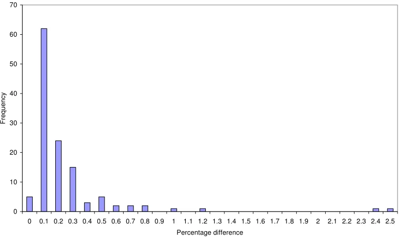
The main potential for computational savings arises in larger network applications. For

illustration, in the Headingley network, a single origin-destination flow was increased by

10%, representing in practice (say) the impact of a small in-fill housing development. The

solutions were compared from two methods: linear approximation from the unperturbed case,

and re-estimation of the equilibrium. The network impact on arc flows is illustrated in Figure

2, with the width of the arc lines representing the absolute increase in flow relative to the base

case. On a 450MHz Pentium II PC, the time to compute the sensitivity expressions was 14

minutes, but subsequently any number of linear-approximated equilibria resulting from

changes to any demand or any travel time function could be computed in negligible time. On

the other hand, re-computing an equilibrium took around 1 minute. Comparing the

approximate and re-estimated solutions on an arc-by-arc level, the average percentage

absolute difference in arc flows was 0.19%, with the largest error only 2.99%. The

distribution of these differences is illustrated in Figure 3. On a network-wide level, the

increase in demand led to a forecast increase in total network travel time of 1.124% by the

linear approximation method, comparing favourably with the forecast 1.118% increase

4.4 Estimating confidence intervals for equilibrium flows

The major items of input data to a traffic network model are the origin-destination trip matrix

and arc travel time functions. In practice, such input data are prone to potentially large

estimation errors, yet typically no effort is made to quantify the impact on the resulting

prediction errors in the model outputs. In statistical terms, a sensible interpretation would

seem to be that the conventional predictions of flows from an equilibrium model are point

estimates of mean flows, but we may reasonably ask for standard errors and/or confidence

intervals for these point predictions. For this purpose, we explore the use of (6) with both ε

and its linear estimator (transformation) assumed now to be random vectors, and with a

given probability distribution representing the sampling error in )

(

* _ε v

ε. For example, in the case

of the origin-destination demand matrix, the sampling error represents the uncertainty in

estimating the mean demands from some given survey data.

Three alternative techniques were tested for estimating output sampling distributions from

given input sampling distributions for the trip matrix and link capacities:

• Re-estimation: Monte Carlo simulation with the full non-linear model: i.e. simulate from

assumed input data sampling distributions, and solve a PSUE for each simulated scenario.

• Linear simulation: Monte Carlo simulation with linear approximation (6): i.e. simulate

from the input data sampling distributions, then use sensitivity expressions (6)−(10).

• Linear analytic: By (6),var

( )

v*(ε) ≈var

(

v*(0)+M-1Nε

)

=M-1Nvar

( )

ε

(

M-1N

)

T is used to

propagate standard errors; and by assuming Normality, confidence intervals are

computed.

These approaches have alternative merits: re-estimation is the most computationally

demanding, using the correct non-linear relationships but being subject to Monte Carlo error;

addition to Monte Carlo error; linear analytic is the most computationally attractive, but is

subject to linearisation error, and must also assume a particular (e.g. Normal) output sampling

distribution.

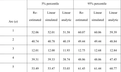
To illustrate each of these techniques, the five-arc network is considered with a (scalar)

origin-destination demand of

q

=

100

+

ε

, where

ε

is a random variable representing the

sampling error in the estimation of the mean demand level. In particular, we assume to be

Normal with zero mean and variance 25 (such an assumption could be justified, for example,

based on a Normal approximation to underlying Poisson demand variation, if the mean

demand were estimated from sampled observations). For both the re-estimation and

linear simulation techniques, 400 realisations of q

ε

4

=

n

were sampled and the empirical 5% and

95% percentiles obtained from the resultant 400 sets of estimated PSUE link flow patterns

corresponding to the sampled demand levels. With the linear analytic technique, the 5×5

arc-flow covariance matrix was calculated using the M and N matrices, with var(ε) =

25.

)) (

var(v* ε

Table 3 shows how the percentiles compare across the three techniques. There is generally

quite good agreement between all three methods. The re-estimation and linear simulation

estimates show the greatest similarity, indicating that the linearisation error is relatively small;

since they are based on the same Monte Carlo draws of the demand, the Monte Carlo effect

can be neglected. Turning attention, then, to a comparison of the linear simulation and linear

analytic techniques, while differences in the estimates produced by the two methods could in

principle be attributable to either Monte Carlo error (in the linear simulation estimates) or

violation of the Normal approximation (made in the linear analytic results), the latter source

may be ruled out in the present case. This is due to the fact that demands have been sampled

from a Normal distribution, and so link flows are linear combinations of Normal variables

can be entirely attributed to Monte Carlo error in the linear simulation estimates. Taken with

the earlier conclusions that linearisation error appears to be small, the overall implication is

that one should place greatest confidence in the linear analytic results, the differences with the

alternative two methods being attributable mainly to Monte Carlo error (this was also

confirmed by re-applying the linear simulation method with an increased number of

pseudo-random draws). While, clearly, the Monte Carlo error can always be reduced by increasing

the number of random draws, there will always be the question of how many draws should be

performed, an issue that does not arise with the linear analytic method.

Further tests were conducted on the three methods (re-estimation, linear simulation, linear

analytic) in realistic networks under various assumptions on the demand levels, input

variation levels, and input sampling distributions (Poisson, Normal, Lognormal). The detailed

results are not given here, but overall a similar pattern in the results was evident to that

reported above. In particular, the difference between the methods in estimating the limits of

95% link flow confidence intervals was seen to be less than 2% (based on 100 Monte Carlo

replications), but both methods which used the linear sensitivity result gave an enormous

saving in computational effort.

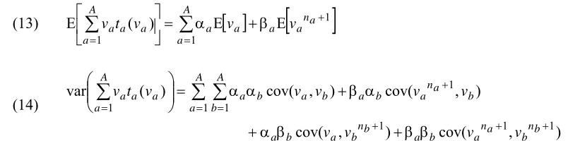
4.5 Estimating a confidence interval for total travel time

The approach described in section 4.4 may be further extended to quantify the uncertainty in

what is a primary practical measure of network performance, total travel time. Suppose the

arc functions are of a form consistent with the commonly used Bureau of Public Roads form

(for other forms, a polynomial Taylor series approximation may be used):

(12) na (

a a a a

a v v

t ( )=α +β n_a ≥0andinteger;α_a ≥0; β_a ≥0; a=1,2,...,A)

(13)

∑

∑

[ ]

[

]

= + = β + α = ⎥ ⎦ ⎤ ⎢ ⎣ ⎡ A a a n a a a a A a a a

at v v v

v 1 1 1 E E ) ( E (14) . ) , cov( ) , cov( ) , cov( ) , cov( ) ( var 1 1 1 1 1 1 1 + + + = = + = β β + β α + α β + α α = ⎟⎟ ⎠ ⎞ ⎜⎜ ⎝ ⎛

∑ ∑

∑

b n b a n a b a b n b a b a A a A b b a n a b a b a b a A a a a a v v v v v v v v v t v

Expressions (13) and (14) are used to exploit knowledge of the link flow covariance matrix

from the linear analytic method of section 4.4. The flow variances and covariances on the

right-hand side of (14) depend on flow moments and cross-moments, and supposing the joint

link flow sampling distribution is approximately multivariate Normal, these required

moments may be computed from standard expressions for multivariate normal moments (e.g.

Isserlis, 1918). By a further Normality approximation for the total travel time sampling

distribution, a confidence interval is thereby computed.

This technique was applied to the Headingley network, assuming there to be sampling error in

the origin destination trip demands. Assuming, for each O-D movement w, Poisson variation

in the underlying flows with mean (approximated, for large by a Normal distribution),

then for a survey based on n independent observations of flows the sampling distribution for

(sample mean flow for O-D movement w) would be approximately Normal with a

variance of

w

q q_w

w

n q_w

[image:26.595.81.483.72.172.2]

. The tests reported here correspond to n = 1, a not unusual case in practice. In

Figure 4, the base situation corresponds to a ‘Demand Multiplier’ of 1 on the horizontal axis.

Other scenarios involve multiplying all O-D matrix elements in the base model by a constant

factor (the Demand Multiplier), which by the Poisson assumption infers an increase by this

factor in both the mean and variance in the underlying O-D flows. On the vertical axis, a

corresponding 95% confidence interval in the total network travel time is illustrated. Clearly,

the width of the interval varies with the demand, an illustration that the magnitude of the

In practice, such confidence intervals may be used in a before-and-after study of some

hypothetical policy measure, in order to test whether the measure is forecast to lead to a

statistically significant improvement in traffic conditions, in the light of the uncertainty in the

forecasts that arises from the uncertainty in the input data. Thus statistical hypothesis testing

may be integrated with the equilibrium analysis of networks, allowing conservative decisions

to be made in the face of uncertainty in the model predictions. Furthermore, such techniques

could also be applied in the context of survey design, such as the problem of determining the

minimum sample size required to achieve a given level of precision. For example, in the

application reported above, one question that could be addressed is: what sample size n is

required when estimating the O-D demand levels, in order that total travel time may be

estimated to within some given level of precision, at a given level of confidence.

On a technical level, it should also be noted that the simple normality assumption adopted

above (for the total travel time distribution) is not critical to the analysis. It may reasonably be

argued that total travel time is much more likely to follow some form of positively skew

distribution, for example. In such a case, more general families of probability densities may

be estimated using higher order moments, using elements of the techniques reported in Clark

& Watling (2004).

4.6 Network Design

The ability to vary ‘design parameters’ of a network in order to optimise a network

characteristic, while anticipating the response of drivers to the changed parameters, is

commonly termed network design. Yang & Bell (1998) review the algorithms known and

adopted by the transportation field for solving such problems. In the continuous network

design problem, the design parameters may, for example, be road widths/capacities, traffic

signal timings or road tolls. For illustration here, we re-visit an example considered by

time functions given in Figure 1 are re-written with constrained design variables

ε

(representing capacity changes) introduced in the flow divisor for each arc:

(15)

4

) ,

( _⎟⎟

⎠ ⎞ ⎜⎜

⎝ ⎛

ε + κ β + α =

α a

a a a a

a

v v

t ε (0≤ε_a ≤4) (a =1,2,...,A)

so that for example, α₁ =4,β₁ =0.6,κ₁ =40. Here, the network design problem has as its

upper level the criterion of total travel time plus a penalty term to reflect the cost of making

changes to the design variables (with below, d₁ =d₂ =d₄ =d₅ =2 and d₃ =1):

(16) Minimise

∑

{

}

subject to

= α

ε +

≡ 5

1

2

5 . 1 ) , ( )

( a

a a

a

at v d

v

f ε ε 0≤ε_a ≤4 (a=1,2,...,5)

which is optimised in our case subject to a lower level PSUE (rather than DUE) relationship:

(17) v is a PSUE given ε,based on arc functions (15).

As noted by Fisk (1984), this problem has the structure of a Stackelberg game (van

Stackelberg, 1952), with the planner ⎯ who is responsible for network changes ⎯ acting as a

‘leader’, and the road users as a collection of ‘followers’ (albeit here with unobserved

components represented as random variables in the road users’ decision process). With (5)

used to represent the lower level (17), the network design problem (16)/(17) has the form of a

bi-level optimisation. The implicit, non-linear, lower level constraints (17) make this a

demanding problem to solve, yet a number of authors have reported success in exploiting

sensitivity analysis information in this context (Yang & Bell, 1998). One potential use of

sensitivity analysis in this context is as a gradient function for the lower level (see the

comments and references to such applications in section 4.1), but we shall continue with the

interpretation of sensitivity analysis as a linear approximation model, particularly exploring

whether a single sensitivity analysis could be sufficient to use throughout the course of the

upper level optimisation. We test this hypothesis on the five-arc network by comparing the

‘optimal’ solution estimated by using a single linear approximation with that obtained by

To solve the example problem, we used Powell’s method (Powell, 1964) for the optimisation,

a well-known gradient-free method, based on two alternative approaches for evaluating the

objective function. In what we shall call the re-estimation method, for a single function

evaluation at a given ε, we solve a full PSUE problem (17), and then substitute the

resulting flows with the given ε into (16). (The random seed was re-set to the same value for

each function evaluation, in order to minimise the potential for problems with Monte Carlo

error in estimating the PSUE solution.) This method thus follows in the spirit (though not the

specific approach) of the study of derivative-free techniques for the network design problem

(Suwansirikul et al, 1987; Friesz et al, 1992). In contrast, with what we shall term the

linearised method, to evaluate at a given ε we use the linear relationship (6) (as an

approximation to (17)), and substitute the approximate flows with the given ε into (16); this

follows in the spirit of the sensitivity-based techniques studied by Bell & Iida (1997). For this

latter method, a single linear approximation ((6) evaluated at ε=0) is deduced before the

optimisation commences. In both the re-estimation and linearised methods, the stopping

criterion used was that the difference between objective function values over successive

iterations should be less than 10 )

(ε

f

) (ε

f

-4_{. An initial condition of ε=0 was used; other initial}

conditions were tested, but did not find other local optima.

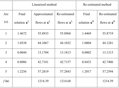
Table 4 presents the results of these experiments. denotes the final solution obtained by the

linearised method. This method crucially assumes the linear approximation about ε=0 to be

valid across the whole feasible region; a check on whether this might be reasonable can be

made by comparing the linear approximate and re-estimated PSUE flows at the final

solution, . This comparison is given in the table, and a close correspondence is observed,

indicating that the linearisation may be reasonable. The final solution from the re-estimation

method, , took around 435 seconds to compute, compared with less than 1 second to

compute . The objective function values produced by the various methods are also given;

L

ε

L

ε

R

ε

L

and for information, the initial value of the objective function is f(0)=1259.70. The final

values of the design variables from the two methods are extremely close, and the resulting

value of the objective function almost identical. It is noted finally that the solutions obtained

here were appreciably different, though the same order of magnitude, as the optimal values

(1.35, 1.22, 0.00, 0.95, 1.08) obtained by Cho & Lo (1999) for the case of DUE.

5. CONCLUSION

The development of network equilibrium methods has been geared towards the efficient

estimation of point solutions at given values of the input parameters. They are much less

suitable for applications in which an explicit relationship is needed between variations in the

input parameters and the model predictions. We have demonstrated that, by using a linear

approximation to this explicit relationship, it is possible to address in a natural way problems

of statistical inference and network optimisation. Direct applications of these techniques

include, for example, the determination of optimal toll levels, hypothesis testing of

before-and-after studies and survey design.

There are many possible directions for further developments of these methods. One such class

of developments involves generalisation of the model, e.g. to account for elastic

origin-destination demand (where the demands are a function of the generalized travel times),

non-separable travel time functions, and multiple classes of traveller.

ACKNOWLEDGEMENTS We would like to thank two anonymous referees for their

REFERENCES

Bell MGH & Iida Y (1997). Transportation Network Analysis. John Wiley &Sons, Chichester

Beckmann MJ, McGuire CB & Winsten CB (1956). Studies in the Economics of

Transportation. Yale University Press, New Haven.

Blum JR (1954). Multidimensional Stochastic Approximation Methods. Annals of

Mathematical Statistics25, 737-744.

Bureau of Public Roads (1964). Traffic assignment manual. US Department of Commerce.

Cantarella GE & Binetti MG (2002). Stochastic Assignment with Gammit Path Choice

Models. In: Transportation Planning: State of the Art (ed. by M. Patriksson & M. Labbé),

Kluwer, Dordrecht, Netherlands, pp. 53-68.

Cascetta E, Nuzzolo A, Russo F & Vitetta A (1996). A Modified Logit Route Choice Model:

Overcoming Path Overlapping Problems. Specification and Some Calibration Results for

Interurban Networks. Transportation and Traffic Theory: Proceedings of the 13th

International Symposium on Transportation and Traffic Theory, ed J.B. Lesort, pp.

697-711, Elsevier Science, Oxford.

Chen A, Chang MS & Yang CY (2001a). Dynamic capacitated user-optimal departure time/

route choice problem with time-window. European Journal of Operational Research132,

603-618.

Chen A, Lo HK & Yang H (2001b). A self-adaptive projection and contraction algorithm for

the traffic assignment problem with path-specific costs. European Journal of Operational

Research 135, 27-41.

Cho H-J & Lo SC (1999). Solving Bilevel Network Design Problem Using a Linear Reaction

Function Without Nondegeneracy Assumption. Transportation Research Record1667,

96-106.

Cho H-J, Smith TE & Friesz TL (2000). A reduction method for local sensitivity analyses of

Clark SD & Watling DP (2000). Probit Based Sensitivity Analysis for General Traffic

Networks. Transportation Research Record1733, 88-95.

Clark SD & Watling DP (2002). Sensitivity analysis of the probit-based stochastic user

equilibrium assignment model. Transportation Research 36B, 617-635.

Clark SD & Watling DP (2004). Modelling network travel time reliability under stochastic

demand. Transportation Research B, in press.

Daganzo CF (1979). Multinomial Probit: The Theory and its Application to Demand

Forecasting. Academic Press, New York.

Daganzo C & Sheffi Y (1977). On Stochastic Models of Traffic Assignment. Transportation

Science11(2), 253-274.

Davis GA (1994). Exact local solution of the continuous network design problem via

stochastic user equilibrium. Transportation Research 28B, 61-75.

Fiacco AV (1983). Introduction to Sensitivity and Stability Analysis in Non-linear

Programming. Academic Press, New York.

Fisk C (1980). Some Developments in Equilibrium Traffic Assignment. Transportation

Research 14B(3), 243-255.

Fisk CS (1984). Game Theory and Transportation Systems Modelling. Transportation

Research 18B(4/5), 301-313.

Frank M & Wolfe P (1956). An algorithm for quadratic programming. Naval Research

Logistics Quarterly3(1/2), 95-110.

Friesz TL, Cho H-J, Metha NJ, Tobin RL & Anandalingam G (1992). A simulated annealing

approach to the network design problem with variational inequality constraints.

Transportation Science 26, 18-26.

Gentile G & Papola N (2001). Network design through sensitivity analysis and singular value

decomposition. Paper presented at TRISTAN IV, San Miguel, Azores, June 13th–19th