T
ECHNIQUES FOR
D
ATA
P
ATTERN
S
ELECTION
AND
A
BSTRACTION
“Thesis submitted in accordance with the requirements of the University of
Liverpool for the degree of Doctor in Philosophy by Konstantinos Nikolaidis.”
ACKNOWLEDGEMENTS
I would like to express my deep gratitude to Dr Goulermas for his invaluable and constructive help regarding this research. His suggestions, support and more importantly his tolerance made everything look easier and enabled me to complete this work, which would have been impossible otherwise. After all these years I spent next to him I consider him more a friend than a supervisor.
I would also like to thank my parents and brother for their encouragement and love throughout my studies. Their support made everything possible. I am also grateful to my grandmothers for their constant support. I also wish to acknowledge the help and support of Helen.
I would also like to express my appreciation to Myrto Pavlini for her love, tolerance and understanding.
Finally, I my special thanks are extended to the following people:
! Eduardo Rodriguez for his valuable advice on Maths and Genetic programming as well as his assistance with the Matlab tool.
! Tingting Miu for her assistance and suggestions on my last piece of work for Chapter 6 of this thesis.
! Elena Marchiori for providing her code of the CCIS algorithm.
! The entire staff of the Electrical and Electronics Engineering Department of Liverpool University for their excellent disposition.
3
ABSTRACT
This thesis concerns the problem of prototype reduction in instance-based learning. In order to deal with problems such as storage requirements, sensitivity to noise and computational complexity, various algorithms have been presented that condense the number of stored prototypes, while maintaining competent classification accuracy. Instance selection, which recovers a smaller subset of the original training set, is the most widely used technique for instance reduction. But, prototype abstraction that generates new prototypes to replace the initial ones has also gained a lot of interest recently. The major contribution of this work is the proposal of four novel frameworks for performing prototype reduction, the Class Boundary Preserving algorithm (CBP), a hybrid method that uses both selection and generation of prototypes, Instance Seriation for Prototype Abstraction (ISPA), which is an abstraction algorithm, and two selective techniques, Spectral Instance Reduction (SIR) and Direct Weight Optimization (DWO).
CBP is a multi-stage method based on a simple heuristic that is very effective in identifying samples close to class borders. Using a noise filter harmful instances are removed, while the powerful heuristic determines the geometrical distribution of patterns around every instance. Together with the concepts of nearest enemy pairs and mean shift clustering this algorithm decides on the final set of retained prototypes.
DWO is a selection model whose output set of prototypes is decided by a set of binary weights. These weights are computed according to an objective function composed of the ratio between the nearest friend and nearest enemy of every sample. In order to obtain good quality results DWO is optimized using a genetic algorithm.
ISPA is an abstraction technique that employs the concept of data seriation to organize instances in an arrangement that favours merging between them. As a result, a new set of prototypes is created.
Results show that CBP, SIR and DWO, the three major algorithms presented in this thesis, are competent and efficient in terms of at least one of the two basic objectives, classification accuracy and condensation ratio. The comparison against other successful condensation algorithms illustrates the competitiveness of the proposed models.
TABLE OF CONTENTS
!"#$%&'(")*+,-*./!/*0/!!"-%*)"1"#!&,%*/%.*/2)!-/#!&,%33333333333333333333334!
/#5%,61".7"8"%!)333333333333333333333333333333333333333333333333333333333333333333333333333333333333333333333333333333333339!
/2)!-/#!33333333333333333333333333333333333333333333333333333333333333333333333333333333333333333333333333333333333333333333333333333333333:!
#$/0!"-*4;*8/#$&%"*1"/-%&%7333333333333333333333333333333333333333333333333333333333333333333333333333333333333333<! 434! &%!-,.(#!&,%3333333333333333333333333333333333333333333333333333333333333333333333333333333333333333333333333333333333333333333<! 439! 0/!!"-%*-"#,7%&!&,%33333333333333333333333333333333333333333333333333333333333333333333333333333333333333333333333333333=! 43:! %"/-")!*%"&7$2,(-*#1/))&+&"-333333333333333333333333333333333333333333333333333333333333333333333333333333333333>! 43?! 0-,21"8*/%.*)#,0"333333333333333333333333333333333333333333333333333333333333333333333333333333333333333333333333333333333@! 43A! 0-/#!&#/1*."B"1,08"%!333333333333333333333333333333333333333333333333333333333333333333333333333333333333333333333 4C! 43<! 0(21&#/!&,%)3333333333333333333333333333333333333333333333333333333333333333333333333333333333333333333333333333333333333333344!
#$/0!"-*9;!&%)!/%#"*)"1"#!&,% 33333333333333333333333333333333333333333333333333333333333333333333333333333333349! 934! &%!-,.(#!&,%333333333333333333333333333333333333333333333333333333333333333333333333333333333333333333333333333333333333333349! 939! ".&!&%7*/%.*#,%."%)&%7*%"/-")!*%"&7$2,(-333333333333333333333333333333333333333333333333333333334:! 93:! %"&7$2,(-$,,.*2/)".*/00-,/#$")33333333333333333333333333333333333333333333333333333333333333333333333334@! 93?! 7-/0$*2/)".*/00-,/#$")3333333333333333333333333333333333333333333333333333333333333333333333333333333333333333333 94! 93A! &%)!/%#"*6"&7$!*1"/-%&%733333333333333333333333333333333333333333333333333333333333333333333333333333333333333339=! 93<! %"/-")!*"%"8D*2/)".*!"#$%&'(")3333333333333333333333333333333333333333333333333333333333333333333333333333:C! 93=! ."%)&!D*2/)".*/00-,/#$")3333333333333333333333333333333333333333333333333333333333333333333333333333333333333333:9! 93>! 8&)#"11/%",()*/00-,/#$")333333333333333333333333333333333333333333333333333333333333333333333333333333333333333:A! 93@! #,%#1()&,%333333333333333333333333333333333333333333333333333333333333333333333333333333333333333333333333333333333333333333333:=!
#$/0!"-*:;*&%)!/%#"*/2)!-/#!&,% 33333333333333333333333333333333333333333333333333333333333333333333333333:>! :34! &%!-,.(#!&,%3333333333333333333333333333333333333333333333333333333333333333333333333333333333333333333333333333333333333333:>! :39! -(1"E2/)".*0-,!,!D0"*8"-7&%7333333333333333333333333333333333333333333333333333333333333333333333333333333:@! :3:! 1"/-%&%7*B"#!,-*'(/%!&F/!&,%3333333333333333333333333333333333333333333333333333333333333333333333333333333??! :3?! #1()!"-&%7*/17,-&!$8)3333333333333333333333333333333333333333333333333333333333333333333333333333333333333333333333 ?=! :3A! #,%#1()&,%333333333333333333333333333333333333333333333333333333333333333333333333333333333333333333333333333333333333333333333A4!
#$/0!"-*?;*/*#1/))*2,(%./-D*0-")"-B&%7*/17,-&!$8 33333333333333333333333333333333 A9! ?34! &%!-,.(#!&,%3333333333333333333333333333333333333333333333333333333333333333333333333333333333333333333333333333333333333333A9! ?39! !$"*0-,0,)".*/17,-&!$8333333333333333333333333333333333333333333333333333333333333333333333333333333333333333333 A:! "#! $%&&'(")*!+,-$$!.&/)0-1"2$######################################################################################################34! ""#! 0"$'")*/"$(")*!.2'522)!.&1021!-)0!)&)6.&1021!")$'-)+2$#######################################34! """#! 71/)")*!.&1021!")$'-)+2$########################################################################################################38! "9#! +,/$'21")*!)&)!.&1021!")$'-)+2$#########################################################################################3:! ?3:! "G0"-&8"%!/1*/%/1D)&)33333333333333333333333333333333333333333333333333333333333333333333333333333333333333333333333 <4! "#! )/%21"+-,!12$/,'$##########################################################################################################################;4! ""#! 0"$+/$$"&)##########################################################################################################################################;<! ?3?! #,%#1()&,%)3333333333333333333333333333333333333333333333333333333333333333333333333333333333333333333333333333333333333333333<@!
5 ""#! 2A721"%2)'-,!-)-,B$"$#################################################################################################################?4! -#! )/%21"+-,!12$/,'$#########################################################################################################################?<! !"! #$%&'%%$()333333333333333333333333333333333333333333333333333333333333333333333333333333333333333333333333333333333333333333333333333 =?! """#! +&)+,/$"&)$#####################################################################################################################################?3! A3?! )0"#!-/1*7-/0$*,0!&8&F/!&,%3333333333333333333333333333333333333333333333333333333333333333333333333333333333=<! "#! .&1021!0"$+1"%")-'")*!=2-'/12$##############################################################################################?;! ""#! .&1021!-)0!)&)6.&1021!")$'-)+2!7-1'"'"&)")*###############################################################8C! """#! 2A721"%2)'-,!-)-,B$"$################################################################################################################8D! "9#! +&)+,/$"&)########################################################################################################################################:4!
#$/0!"-*<;*0-,!,!D0"*-".(#!&,%*2/)".*,%*.&-"#!*6"&7$!*
,0!&8&F/!&,%33333333333333333333333333333333333333333333333333333333333333333333333333333333333333333333333333333333333333333333333@?! <34! &%!-,.(#!&,%3333333333333333333333333333333333333333333333333333333333333333333333333333333333333333333333333333333333333333@?! <39! !$"*0-,0,)".*/17,-&!$8333333333333333333333333333333333333333333333333333333333333333333333333333333333333333333 @A! "#! ")$'-)+2!52"*('!%&02,,")*########################################################################################################:3! ""#! &7'"%"$-'"&)!71&+20/12##############################################################################################################:?! """#! 721=&1%-)+2!-++2,21-'"&)!(2/1"$'"+$###############################################################################:?! <3:! "G0"-&8"%!/1*/%/1D)&)33333333333333333333333333333333333333333333333333333333333333333333333333333333333333333333333 @@! "#! )/%21"+-,!12$/,'$####################################################################################################################### @C4! ""#! 0"$+/$$"&)####################################################################################################################################### @C4! <3?! #,%#1()&,%)3333333333333333333333333333333333333333333333333333333333333333333333333333333333333333333333333333333333333333 4C>!
#$/0!"-*=;*"0&1,7(" 33333333333333333333333333333333333333333333333333333333333333333333333333333333333333333333333333333 44C! =34! #,%#1()&,%)3333333333333333333333333333333333333333333333333333333333333333333333333333333333333333333333333333333333333333 44C! =39! +(!(-"*6,-53333333333333333333333333333333333333333333333333333333333333333333333333333333333333333333333333333333333333 449!
C
HAPTER
1:
M
ACHINE
L
EARNING
The purpose of this chapter is to provide a broad overview of the field of Machine learning. This section emphasizes on instance-based learning, and more specifically on non-parametric methods for classification using the nearest neighbour rule. Section 1.1 briefly describes the concept of Machine learning and its applications. Section 1.2 provides a small introduction to the pattern recognition problem in machine learning. Section 1.3 is a brief summary of the various types of classifiers that exist and introduces the Nearest Neighbour (NN) classifier, which is used throughout this work. Finally, section 1.4 presents the problems that arise in instance-based learning and are related with the use of NN, and explains the rationale behind this PhD study.
1.1
Introduction
7 as statistics, probability theory, information theory, optimization and control theory, but also it expands to other scientific areas like philosophy and archaeology [Miu08].
Machine learning appears in many aspects of modern day life as it has a very wide range of applications. From simple examples such as web page ranking in search engines and automatic translations to rather complex applications such as medical diagnosis and bio-informatics, machine learning is successfully applied. It is actively used the last few years for security purposes, i.e. face recognition or verification, fingerprint recognition or credit card fraud [Smo10]. Other applications that involve machine learning are financial such as stock market analysis and direct marketing, robotics, computer games, image processing, speech or handwriting recognition and failure detection.
1.2
Pattern Recognition
The problem of pattern recognition has been the focus of research for many years, and while initially it was mostly on a theoretical basis the development of machine learning algorithms enabled the use of it on cutting edge practical applications. Bishop [Bis06] described machine learning algorithms as a function !(x), which takes an input vector x and generates an output vector y of the same form as the target vector. Machine learning algorithms consist of two distinct stages, the first one being the training phase. During this stage, the model uses the input vectors to train its parameters according to the learning function !. The key objective of the learning process is the ability of the model to generalize, meaning to extract general information from the inputs that enables it to correctly treat unknown data patterns. Once the learning process ends, the model proceeds to the testing phase. The algorithm is then tested on new unknown samples that determine the generalization capability of the model.
the other hand, the output of a classification problem is a class label that represents the category of the pattern.
More precisely, pattern classification is a formulation of supervised learning whose goal is to accurately predict the class labels of unseen patterns. The decision making of the model is driven by the training data supplied to the algorithm. Given a set of n labeled training samples
!
X
=
{
x
1,
x
2,...,
x
n}
"
R
d, where Rd is the d-dimensional real feature space, and each sample is associated with a unique class label!
"
( )
x
#
L
=
{
l
1,l
2,...,
l
c}
, with c being the number of classes, the objective of a classification algorithm is to construct a functional mapping!
"
:
R
n#
L
so that any unseen sample xi is correctly assigned to a class label li. Pattern classification can be sorted in binary and multi-class classification. Binary classification is the task of classifying the input samples into one of two possible sets, whereas the latter can assign a pattern to one of multiple classes. In order to simplify the multi-class problem, in some cases, one can consider it as a series of binary problems. Although many consider them two different tasks, no distinction between binary and multi-class classification is made in the experiments and implementations of this study.1.3
Nearest Neighbour Classifier
Despite the fact that pattern recognition is a relatively new science, various classifiers have been introduced. A large group of classifiers, namely linear classifiers, are designed to classify data regardless of the underlying distribution of the training patterns. In this case, the decision surface is considered to be a linear function of the unknown pattern x. Linear classifiers are known for being relatively simple and computationally inexpensive [The99]; such models are linear discriminant functions like [Fis36], [Zha10a], which are used in various applications [Yu08], and the perceptron algorithm [Hay99]. For more complicated case where classes are non-linearly separable the use of non-linear classifiers is required. Some examples of such algorithms are the multi-layered perceptron methods [Hay99] and the radial basis function network [Hay99] or the decision trees [Sug06]. Another approach involves the classification of patterns based on the probability of it belonging to a certain class. These classifiers depend on the probability distributions of the training patterns; some representative algorithms are the maximum likelihood parameter estimator [Kay93], the parzen windows approach [Bab96] and the nearest neighbour classifier [And02].
9 based learning algorithms to perform supervised non-parametric classification. It is widely used in machine learning because of its simplicity and the fact that its error probability is bounded by twice the Bayes error rate. All instances of the training set are represented by position vectors in a multidimensional feature space, and the k-Nearest Neighbour rule (k-NN) classifies unseen samples based on their closest k instances and requires k being a positive integer. In its simplest form, where k=1, the output value is simply the class of the nearest neighbour. Otherwise, the pattern is assigned to the class of the majority of its k nearest neighbours. Hence, in order to avoid ties between classes, k is usually chosen as an odd number. Despite the fact that k-NN is a learning method that can be used for regression as well, it is utilized only as a non-parametric classifier in this PhD study.
1.4
Problem and Scope
Algorithms that use the NN rule, and instance-based learning methods more generally, suffer from two principal issues. Firstly, a major concern is storage requirement because of the need to store the entire dataset in some type of memory. Secondly, the increased time complexity from having to search large portions of the stored prototypes, in order to predict new queries. The larger the dataset used the higher the response time of the algorithm. Apart from these, a third concern is the noisy instances present in the database. Along with the entire training set noisy instances are also stored, thus degrading accuracy and overall performance of the algorithm.
In order to tackle these drawbacks, rapid advances have been made in the field of data condensation, with the development of numerous methods that target in reducing the training set size, while keeping the error rate as low as possible. Hence, the problem in instance reduction is to determine a set of
!
m
<<
n
=
X
prototypes using the original training set!
condensation, in an attempt to optimise both objectives of accuracy and condensation together. Which type is used depends on the focus of the application. If the creation of new samples to fill regions in the domain of the problem to improve weak representative samples in the original dataset is prioritised, the latter type is preferred. Otherwise, if the preservation of the geometric and discriminative characteristics of the original instances is prioritised, the former type is preferred. Also, instance selection methods are usually much faster.
The wide range of algorithms developed to deal with the issues related to instance-based learning show how significant the problem is. As a result, many works including [Jan04a, Jan04b, Wil00], have analysed and compared various instance reduction techniques. A clear distinction should be made between instance reduction, with which this thesis is concerned, and dimensionality reduction. Considering a dataset as a matrix, instance reduction decreases the number of the rows of the matrix (attributes), while dimensionality reduction deals with the columns (features) of the matrix.
The aim of this thesis is two-fold. Firstly, to solve the problem of instance-based learning using new alternatives. This is achieved by introducing novel techniques for instance reduction. Secondly, to contribute in the field of machine learning not only theoretically, but also practically. In order for the developed algorithms to be successful, they should involve innovative aspects, but they should also be effective. Therefore, the proposed techniques should account for improvements and enhancements in terms of the required objectives, when compared to already known methods in the literature.
In chapters 2 and 3, an investigation of previous work done on the field of instance selection and abstraction is presented and a thorough analysis of each method is performed. This thesis identifies the important aspects of data condensation, based on which it proposes some novel techniques for prototype reduction. These techniques are presented in chapters 4, 5 and 6. The epilogue recapitulates the contributions and advantages of the proposed algorithm, while it discusses possible improvements along with new topics for research.
1.5
Practical Development
11 reduction techniques. Some of these algorithms were implemented by the author of this thesis, while their respective authors provided others. The software tool used to develop the algorithms and obtain all experimental results was Matlab.
1.6
Publications
• Nikolaidis, K., Rodriguez, M.E., Goulermas, J.Y., and Wu, Q.H., 2010. “Instance
seriation for prototype abstraction.” In Proc. of IEEE 5th BICTA International Conference, Liverpool, pp. 1351-1355.
• Rodriguez, M.E., Nikolaidis, K., Goulermas, J.Y., Ralph, J.F., and Miu, T., 2010. “Collaborative projection pursuit for face recognition.” In Proc. of IEEE 5th BICTA International Conference, Liverpool, UK.
• Nikolaidis, K., Goulermas, J.Y., and Wu, Q.H., 2011. “A class boundary preserving algorithm for data condensation.” Pattern Recognition, vol.44, pp. 704-715.
• Nikolaidis, K., Rodriguez, M.E., Goulermas, J.Y., and Wu, Q.H., 2012. “Spectral graph optimization for instance reduction.” IEEE Trans. Neural Networks, vol. 23, pp. 1169-1175.
• Rodriguez, M.E., Nikolaidis, K., Miu, T., Ralph, J.F., and Goulermas, J.Y., 2012. “Towards collaborative feature extraction for face recognition.” Natural Computing, vol.11(3), pp. 395-404.
C
HAPTER
2:
I
NSTANCE
S
ELECTION
The aim of this chapter is to accurately describe the field of prototype reduction, more specifically instance selection algorithms, and provide a thorough analysis of various existing methods in the literature. Section 2.1 briefly describes the concept of instance selection and its processes. Section 2.2 describes instance selection algorithms that are based on the use of the nearest neighbour concept. In section 2.3 methods that define the relative neighbourhood of prototypes are presented. Section 2.4 is an extensive analysis of various graph methods used for prototype reduction. In 2.5 algorithms using instance weight learning for instance selection are described, while section 2.6 demonstrates the developments on nearest enemy-based techniques for instances reduction. Section 2.7 investigates instance-based techniques that use density estimation as the main tool for condensation. Finally, section 2.8 presents some novel prototype selection algorithms that employ unusual means, such as evolutionary computation or projection of samples to new dissimilarity spaces.
2.1
Introduction
13 existing in the training set. Prototype selection methods can be further subcategorized to editing algorithms, that aim to improve classification accuracy by removing harmful instances, condensation techniques that focus on discarding superfluous instances, and hybrid methods, which are a combination of the other two, and demonstrate highly competitive performances since they deal not only with noisy but redundant prototypes as well [Gar10].
Classification involves the use of a training set X of preclassified instances, and a testing set of unseen samples. In instance selection algorithms, during the training process, a small subset of X is selected and applying the k-NN classifier it is used to predict the class labels of all samples in the testing set. As already mentioned no artificial
prototypes are generated; Hence, having an initial set
!
X
=
{
x
" #
d}
of n d-dimensionalinstances, where each sample is associated with a unique class label
!
"
( )
x
#
L
=
{
l
1,...,
l
c}
, the problem in instance selection is to determine a set of mrepresentative prototypes from X (where m << n) that best describes the initial distribution.
2.2
Editing and Condensing Nearest Neighbour
One of the simplest editing rules is the Editing Nearest Neighbour (ENN), proposed by Wilson in 1972 [Wil72]. Given a set of n labeled instances, Wilson used the k nearest neighbour rule to reach a decision for every instance and filter the original training set. His method selects an instance xi from X and its k nearest neighbours are computed. The class of xi is determined by the class of the majority of its k nearest neighbours, and whenever a tie occurs, random selection is used to assign the class. In case of misclassification, xi is removed from the original set X. Hence, ENN is an iterative algorithm and the final subset contains only instances that are correctly classified by their k-NN. As a result, noisy samples are removed resulting to the improvement of the classification accuracy.
CNN aims to preserve the classification accuracy already achieved by selecting instances of the training set that correctly classify the rest.
CNN has the disadvantage that much depends on random selection. Therefore, many algorithms were prompted by it, in search of the optimum subset S. One such algorithm is the Reduced Nearest Neighbour (RNN), which enhances data condensation by removing redundant instances [Gat72]. After the application of CNN every prototype xi in S is tested and if its removal results in no miss-classifications in X, xi is considered superfluous and permanently discarded. Although RNN highly reduces the size of the original set, it does not guarantee a minimal output set.
Another instance selection technique is the Selective Nearest Neighbour (SNN) proposed in [Rit75], which retains instances close to the class boundaries. SNN rule states that every instance xi of the original training set has to be closer to a same class (friend) instance of the output subset than to any other enemy instance. In order to achieve this, a binary n ! n matrix A is constructed, such that:
!
A
ji=
1
if x
j"Y
i0
if x
j#Y
i$
%
&
(2.1)where Yi is the set of all friend instances of xi that lie closer than its nearest enemy. Some rules for deletion of rows and columns of A are then applied to obtain the final subset. Although this method can display competitive results, the use of A largely increases its complexity compared to methods such as CNN and RNN.
Based on the SNN algorithm, another method was developed to decrease the computational complexity of the nearest neighbour classification. The Modified Selective Subset (MSS) introduced in [Bar05]. The proposed algorithm is similar to SNN with a slight modification on the Yi set, which drives MSS to select instances that lie closer to the class boundaries. Consequently, the main purpose of MSS is not a minimal consistent subset like SNN, but rather a more accurate representation of the initial class borders.
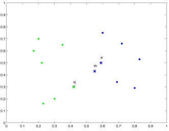
15 Figure 2.I- A two class two dimensional example. For an instance xi the OCNN algorithm successively computes its nearest enemy xj and the same-class border prototype xk.
Chidananda introduced another method for instance condensation using the concept of mutual neighbourhood [Chi79]. The proposed technique is based on the CNN algorithm with the major difference being its initialization. The Mutual Neighbourhood Value (MNV) of every sample is determined, which is computed with respect to the nearest enemy of every instance. The initial prototype that is selected and moved to an initially empty set S is the one with the lowest MNV. Each sample remaining in the original set is then classified according to S, and only misclassified instances are maintained. This process, similar to CNN, ends only when the final output set can classify all instances successfully. During the second stage of the algorithm an evaluation of the remaining instances takes place. Hence, to deal with redundant samples, an instance xi is eliminated from S if its removal results in no misclassifications. When all instances are treated, the algorithm terminates and the final subset contains highly informative samples that are close to the class boundaries.
instance is checked and, if it can be classified correctly by the remaining prototypes of S is discarded. According to Wilson [Wil00], this algorithm is extremely sensitive to noise compared to RNN. From the three methods proposed, IB3, which is also an additive algorithm, is the most effective. Only instances that can be characterized as acceptable are moved in to S. An instance xi is retained if it is not classified correctly by its nearest acceptable instance. The confidence interval that determines acceptability is defined as:
!
p
+
z
22
r
±
z
p p
(
"
1
)
r
+
z
24
r
21
+
z
2r
(2.2)
where z is the confidence factor1, r is the number of classification attempts of the given instance of S, and p is the classification accuracy based on n. An instance is considered acceptable and retained by IB3 if its accuracy is higher than the upper bound of the confidence interval. While every instance that has lower acceptability than the lower limit is removed immediately from S, if an instance is within the confidence interval it is not discarded until the very end of the process.
Another algorithm, called Fast Condensed Nearest Neighbour, was recently proposed in [Ang07a], which discards redundant and harmful instances to largely reduce the size of the training set X. FCNN uses a subset S, which in the initial state holds the centroids of the classes of X. For every instance xi of S, FCNN denotes two sets A and B, where A contains all Voronoi neighbours of xi, i.e. instances that are closer to xi than to any other prototype in S, while B holds the Voronoi enemies of xi. During each iteration a representative instance from B, with respect to xi, is inserted in S and sets A and B for all instances are updated. This procedure continues until all elements of S have no Voronoi enemies, meaning B is empty for every xi belonging to S. In the specific work, two different rules to update S are analysed, depending on the way of selecting the representative sample. In the first case, FCNN1 selects the nearest neighbour of xi in B, while in the other case the centroids of B are selected. The latter algorithm is called FCNN2. Additionally, two rules, the triangle inequality and k-Nearest Neighbour, are used, in order to further reduce the computation time and error rate of the algorithm respectively. FCNN is another instance selection method that discards centre instances; hence, S consists mainly of instances close to the decision boundary. In order to further improve the performance of Fast Condensation Nearest Neighbour, a new method of condensed nearest neighbour was introduced in [Ang07b], the Parallel FCNN. In this case, the entire training set is divided in k subsets X1, X2…Xk that are then assigned to one of k parallel nodes P1,…, Pk. Each node uses the FCNN algorithm described before to
17 reduce the number of instances. Computational time required is then reduced as all nodes can communicate with each other to compute the final training set S.
[image:17.595.155.477.369.623.2]The modified condensed nearest neighbour (MCNN), which is also an instance reduction method based on Hart’s algorithm, was proposed in [Sus02]. MCNN initializes a subset S of the original set X, holding just one instance as a representative prototype for each class. Two different cases have been proposed for selecting the initial representatives, either by computing the sample mean of each class and then selecting the closest prototype to the computed value or by selecting the centroids of every class (as seen in Fig. 2.II). The entire set of instances is then classified according to the representative prototypes and all misclassified instances are moved to another set, from which new representative are selected using the same method as before. S is then updated and the training set is once more evaluated in a similar manner until all samples in the training set are classified correctly. The MCNN algorithm also includes a deletion operator to further improve its performance. So every prototype in the final subset S is evaluated and the ones found superfluous are discarded, leading to an even smaller output subset.
Figure 2.II- A two class two dimensional example similar to the one used in Fig. 2.I. The representative prototypes of the two classes are indicated by “!”.
18
!
x
i"
x
z+
#
<
x
i"
x
j (2.3)where xz is a same class instance and xj represents instances of other classes !(xj)"!(xi). This method is simplified to CNN if #=0, and is further enhanced in [Cho06]. The second method described, involves a matrix manipulation similar to Gates proposal in [Gat72] with the addition of the ‘dead-zone’ threshold.
In 2006 another data reduction method based on condensed nearest neighbour was presented, Generalised CNN [Cho06]. GCNN aimed to select a smaller subset S of the initial training set using an implementation very similar to the one introduced in [Har68]. In Condensed Nearest Neighbour an instance xi is retained as long as:
!
x
i"
q
"
x
i"
p
>
0
(2.4) where p is the nearest same-class prototype and q is the nearest different-class prototype of xi. In the case of GCNN the rule to retain a prototype is modified as follows:!
x
i"
q
"
x
i"
p
>
#$
nfor
# %
[0,1)
(2.5) where !n is the minimum distance between prototypes of different classes. It is obvious that CNN is a special case of GCNN for "=0. The algorithm randomly selects a prototype from each class in order to initialize S, and then the process is similar to CNN as all samples are checked individually with the misclassified ones being moved to a new set. From this set a new prototype for each class is selected and added to S. The process, as explained, is iterative and terminates when all prototypes of the original set are correctly classified. It should be mentioned that the selection of the prototype to be moved in S can be done either randomly [Cho06], or according to a specific rule (such as centroids or mean of samples) [Sus02].A density-based reduction algorithm for identifying and removing outliers was proposed in [Cao08]. This method defines a score for every instance in the training set, the density-similarity-neighbor based outlier factor (DSNOF), which is a measure of how much an instance is considered an outlier. According to this value computed, harmful instances are recognized and discarded. During the first step of the algorithm the k-distance2 neighbours of every instance
!
xi"X and its density are determined.
!
D
(
x
i)
=
N
k(
x
i)
kd
(
x
i)
(2.6)Where D is the density, kd is the k-distance of xi and
!
N
k(
x
i)
is the size of the k distance neighbourhood. DSNOF constructs the similar density series (SDS) of xi in a matrix that consists of its similarity neighbours in descending order. In order to compute the DSNOF of an instance xi, the average series cost of xi has to be calculated:# K-distance of a point
!
x
"
X
is the distance d(x,o) between x and an instance in X such that: 1) For at least k points!
o'"X\
{ }
x it holds that!
d(x,o')"d(x,o) #$ For at most k-1 instances
!
19
!
ASC
(
x
i)
=
d
(
ao
k)
k
k=1n
"
(2.7)where d(aok) is the distance between two adjacent instances in SDS. The final step is the calculation of DSNOF, which is expressed as:
!
DSNOF
(
x
i)
=
N
k(
x
i)
ASC
(
x
i)
ASC
(
o
)
o"Nk(xi)#
(2.8)DSNOF is the probability of a data point being an outlier, hence, instances with high such values, which exceed a certain threshold set by the user, are considered outliers and can finally be removed.
2.3
Neighbourhood based Approaches
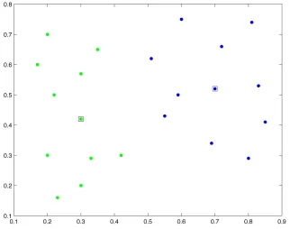
In the nearest neighbour approach only the distance between instances is taken into consideration to define the relative neighbourhood. On the contrary, two new methods introduced in [Cha96], the Nearest Centroid Neighbourhood (NCN) and Nearest Mean Neighbourhood (NMN), use not only closeness but also symmetry to define the neighbourhood of a prototype. During the first step of the process the nearest neighbour of xi is determined, xj, and the centroids Mjk of xj and every other instance xk of the remaining training set
!
X "
{
xi,xj}
are computed. The instance xz, which produces theclosest centroid to xi, in terms of Euclidean distance, is the one selected to define the Neighbourhood. In order to resolve ties, the instance that lies the farthest from the neighbour found previously is selected. As a result, the algorithm determines the neighbours that lie symmetrically around an instance, and spread in all directions as illustrated in Figure 2.III(a). In a similar manner to NCN, instead of computing the centroids between instances, NMN chooses the median to determine the neighbourhood of each instance in the training set.
This neighbourhood-based technique can be efficiently employed for data reduction as proposed in [Loz03], where the geometrical distribution of every instance is determined by computing its Nearest Centroid Neighbourhood. The neighbourhood of every prototype includes all instances computed by the NCN algorithm until its nearest enemy is reached. Then for every region of same class instances, a sample
!
xi"X is
neighbourhoods, in case any of the removed instances contribute to more than one neighbourhood. The algorithm terminates when all instances of the entire training set are treated. But, in order to further improve the classification capability of the model and accurately deal with the problem of border instances being removed, some additional steps were introduced. At the end of the process the condensed training set is used to classify the initial training set, and all misclassified instances are added to the final subset. There is also a second variation of the described method, which instead of selecting a representative prototype for each neighbourhood computes its centroid. As a result, the output of this method is a reduced set of newly generated prototypes.
[image:20.595.116.510.248.413.2](a) (b)
Figure 2.III- A two class two dimensional example. (a) NCN of a sample pattern x defined by the same-class instances indicated by “!”. (b) Neighbourhood of instance xi after Lozano’s method has been applied.
21
!
"
(
x
i,
x
j)
=
HVDM
(
x
i,
x
j)
#
s
(
x
i)
(2.9)where s(xi) is the similarity of the representative of Ni and HVDM is the Value Difference Metric described in [Sta86], and xj is assigned to class of the representative prototype that provides minimum score value ". So space is partitioned into neighbourhoods and search is performed only within the representatives and not through the entire training X.
A nearest neighbour method that computes local neighbourhoods for classification was introduced in [Dom02]. The adaptive metric nearest neighbour algorithm (ADAMENN) proposed a new distance metric, the Chi-squared distance, which is capable of producing more homogeneous neighbourhoods. ADAMENN is an adaptive algorithm for pattern classification. Similarly, another adaptive metric technique for producing neighbourhoods was presented in [Has96]. In this case linear discriminant analysis was used to determine the suitable metric. In general, neighbourhoods and neighbourhood relations are very important concepts in the field of machine learning. Initially, topological algorithms that deal with neighbourhood spaces were designed to operate merely as classifiers, such as [Owe84] and [Sal91], or distance metrics [Wei09], in order to exceed the performance of other local classifiers as the k-NN rule. However, neighbourhood based techniques are now considered a very powerful tool that is widely used in various applications of machine learning, such as instance reduction, which has already been presented in this section, or for feature selection [Hu08].
2.4
Graph based Approaches
Figure 2.IV- Voronoi polygons [cs.sunysb.edu]
Another method equivalent to Voronoi diagrams is Gabriel graphs, which are formed when two Gabriel neighbours are connected with an edge. Two points xi and xj, are Gabriel neighbours when the disk having line segment xixj as its diameter contains no other points. This method is used in the Hybrid Gabriel-Graph algorithm introduced in [Bha05]. In order to compute the Gabriel neighbours of the samples in the training set, a framework called GSASH, Gabriel spatial approximation sample hierarchy, is proposed by Bhattacharya. GSASH is a graph, at which every node corresponds to a data item and nodes that are Gabriel neighbours are connected by an edge. The original training set is edited in the beginning by using Gabriel neighbours, so instances that are misclassified by their Gabriel neighbours are permanently discarded. This is a technique based on Wilson’s editing method [Wil72]. After filtering, in order to remove redundant instances from the training set, all samples that their Gabriel neighbours belong to the same class are removed. During the third and final step of the algorithm, the iterative case filtering (ICF) algorithm [Bri02] is used on the reduced training set to obtain the final output subset. So, instead of the k-NN method GSASH uses Gabriel neighbours to classify all new samples.
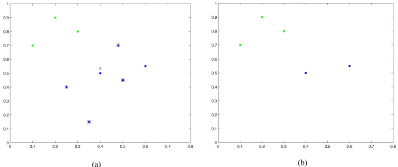
In [Muh03], the geometrical neighbourhood of every instance xi of X is determined using the Relative Neighbourhood Graph method [Tou80] and instances belonging to different classes are either discarded or relabeled. This editing technique is very efficient for noise and outliers removal, because it uses cutting edge weights to decide whether an edge between two instances should be cut or not (Fig. 2.V). For an instance xi belonging to a class li the matching null hypothesis, which is the probability of an instance in the neighbourhood of xi not belonging to the same class, is defined as:
!
H
o=
1
"
p l
( )
i (2.10)23
!
J
i=
w
ijI
i(
j
)
j=1 Ni
"
(2.11)where k is the number of instances in the neighbourhood of xi, wij is the weight of the edge between xi and xj and I are independent and identically distributed random variables, according to Bernouilli law [Muh03]. Based on the value of J under the null hypothesis samples can be optimized as good, doubtful or bad and thresholds are set in order to distinguish between them. When all instances of the training set are evaluated, bad and doubtful ones are selected and checked individually. From these instances, the ones that have good instances lying within their neighbourhood are optimized according to the majority of their k-nearest neighbours, while samples with no good instances within their k-NN are discarded. This method tries to condense the training set and simultaneously increase class separability.
(a) (b)
Figure 2.V- A two class two dimensional example. (a) The Relative Neighbourhood graph is depicted. The edges between the two classes are cut off.
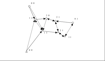
Another graph-based algorithm is Hit Miss Networks (HMN). These ‘networks’ are directed graphs of instances in the training set [Mar08]. For every sample, the nearest neighbours from all classes are determined and an edge between the sample and its neighbours is defined; a hit edge is an edge between instances of the same class, while a miss edge is defined if instances belong to different classes. As a result, every instance of X has a number of outgoing edges equal to the total number of classes. A hit and a miss degree are computed for every node of the training set, as can be observed in Fig. 2.VI. Based on the hit and miss degrees computed by the HMN algorithm, the following deletion criterion is applied:
!
Figure 2.VI- Hit Miss Network of a two class two dimensional data set. The two numbers next to each sample pattern indicate its respective hit (solid lines) and miss (dash lines) degrees.
This rule tends to discard isolated instances with zero hit degree, along with noisy instances. HMN can lead to the removal of a very large number of instances that may cause a drop in the classification accuracy of the algorithm. Thus, to avoid large losses of important information, three different heuristics are employed. Firstly, a threshold is set for the number of vectors belonging to each class. If this number falls below the threshold set, all discarded instances of the specific class with hit degrees greater than zero are restored. A second heuristic involves multi-class training sets (more than 3 classes). All instances that have non-zero hit degree along with a small valued miss degree are restored. The threshold proposed in [Mar08] is
!
L
2 . Finally, a threshold is set for every
class and instances with a greater number of hit edges than the 25% of their own class are retained. These instances are likely very close to the class centers contributing to cluster identification.
Based on HMN two other algorithms, Class Conditional Instance Selection (CCIS) [Mar10] and Laplace Instance Filtering (LIF) [Mar09] have been introduced. The first method is an enhanced version of HMN that makes use of two directed graphs, the within-class graph
!
G
wc=
(
V
,
E
wc)
, which is for same class instances and the edge matrix for a vertex v is defined as:!
E
wc=
{
u
"
X
:
#
( )
u
=
#
( )
v
,
u
"
1
NN v
( )
}
(2.13) and for enemy instances the between-class graph!
G
bc=
(
V
,
E
bc)
that is defined in a similar manner with an edge matrix:0 1
1 1 2 1
2 0 0 0
1 2
2 1 1 3
[image:24.595.110.538.65.316.2]25
!
E
bc=
{
u
"
X
:
#
( )
u
$
#
( )
v
,
u
"1
NE v
( )
}
(2.14) where NE(.) defines the nearest enemy of v. Using the Kullback-Leibler divergence [Lin91],!
K p
(
1,
p
2)
( )
v
=
p
1( )
v
log
p
1( )
v
1
2
(
p
1( )
v
+
p
2( )
v
)
(2.15)
where p1(.) and p2(.) are two discrete probability distributions over X. Denoting by pw(.) and pb(.) the within and between-class degrees of a vertex divided by the total in degree of Gwc and Gbc respectively, the final class conditional score is given by:
!
CCS v
( )
=
K p
(
w,
p
b)
( )
v
"
K p
(
b,
p
w)
( )
v
(2.16) So, CCIS displays negative scores for instances that contribute more to the between-class divergence and retains the ones with higher scores. This algorithm demonstrates considerable improvement in the condensation capability compared to its predecessor HMN.On the other hand, the latter algorithm, LIF, is of significant importance as it is the first method to introduce Laplacian graphs to instance selection. So, the Laplace score is defined as the discrete Laplace operator for the between-class graph acting on the degree function of the within-class graph. For a vertex u in the between-class graph connected to the set of vertices v, the Laplace score is defined as
!
L
( )
g
( )
u
=
1
d u
( )
g u
( )
d u
( )
"
g v
( )
d v
( )
#
$
%
%
&
'
(
(
u~v)
(2.17)where
!
d u
( )
is the degree function in the between-class graph and is the degree of the given vertex in the within-class graph. The above equation can be rewritten in matrix notation as!
L
( )
g
=
L
BCW
WC1
n"1 (2.18)where is the normalized Laplacian matrix for the between-class graph,
!
W
WC is affinity matrix for the within-class graph, and is a column vector with all its elements equal to one. The normalization of the Laplacian matrix is performed so that the rows of the affinity matrix sum to one. Therefore,!
L
BC=
I
"
D
BC"1 2W
BCD
BC"1 2=
1
if
u
=
v
"
1
d u
( )
d v
( )
if
u
~
v
Based on the computed score, similar to HMN, a deletion criterion is employed to make a decision for every instance, with samples displaying negative values being removed from the training set. The basic application of the LIF algorithm is to identify and remove outliers since it operates as a noise filter.
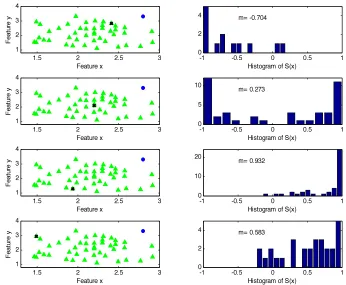
A k-nearest neighbour model that uses a weighted sum of the influence of different classes on instances is proposed in [Hua07]. This method determines the neighbourhoods N that accurately represent the entire training set
!
X =
{
x1,...xi,...xn}
"Rd. After normalising all the input samples, a threshold # and a
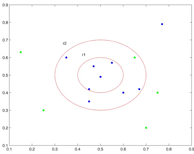
density control value p are set, as well as a ‘0’ tag that is assigned to every instance. This threshold represents the maximum acceptable value of noise allowed in a neighbourhood, as can be seen in Figure 2.VII. The next step of the algorithm is the computation of the density of every class li:
!
p
i=
m
i2
n
(2.20)where mi is the number of instances belonging to the specific class. Choosing an instance xi with a ‘0’ tag, the algorithm performs a search of its nearest neighbour that does not satisfy the following condition:
!
k(l
i)
r
"
p
ip
(2.21)where k(li) is the number of instances belonging to class of xi, r is the radius from point xi and p is the density of the region determined. The neighbourhoods N that satisfy condition (2.22) are chosen as representative candidates, otherwise the tag of xi becomes ‘-1’.
!
1
"
d x
(
i,
x
j)
r
#
$
%
%
&
'
(
(
xj)ci*xj+Ni*xj+X
,
1
"
d x
(
i,
x
j)
r
#
$
%
%
&
'
(
(
j=1,j-i n
,
(2.22)
The candidates found are then scanned to determine the one with the largest number of instances that is set as the class representative3, while all instances covered by it are tagged as ‘1’. The algorithm terminates when all instances are treated, while new samples are classified with respect to the computed representatives instead of the original set of instances.
27 Figure 2.VII- The different radii define different error zones. r1 indicates a zero error allowance. r2 defines an area where a certain amount of noise is permitted.
2.5
Instance Weight Learning
Instance weight learning (IWL) is a form of lazy learning, which has been used not only for regression, dimensionality reduction and various other applications, but also for noise and outlier removal, as well as for prototype reduction [Atk97]. In IWL different weights w with
!
w
i"
R
d, are assigned to every instance xi of the original set
!
X =
{
x1,...xi,...xn}
"Rd, and as explained in [Kan08] these weights show if and how important an instance is. Although the majority of these methods employ IWL on the distance metric in order to improve the classification error of the k-NN algorithm like [Fer07], [Par06a], there exist some cases where IWL has been used directly for prototype reduction. An example of such a method is the adaptive distance metric proposed in [Ric99], where misclassified prototypes are moved towards the right class. An asymmetric weight is assigned to each prototype of the subset and nearest neighbour classification is applied using a local asymmetrically weighted similarity metric (LASM):
!
"
(x, y)
=
w
i(x, y) x
i#
y
2 i=1d
$
%
&
'
(
)
*
(2.23)A subset of the original set is selected and two functions, reinforcement R and punishment P, are defined. Weights are assigned and can be defined as:
!
w
i(
x,y)
=
w
i0
(x)
if
y
"
x
iw
1i(
x)
otherwise
#
$
where w is the weight, xi is the prototype and y is the query. Weights are initialized in the beginning and a test sample y is selected. Then the nearest neighbour prototype xi of sample y is determined and if both belong to the same class R(.) is used, otherwise P(.) is applied. The reinforcement and punishment steps are expressed as:
!
R
i0w(x), x, y
(
)
=
w
i0
(x)
"
aw
i0(x) x
i
"
y
if y
<
x
iw
i0(x)
if y
#
x
i$
%
&
(2.25)!
R
i1(
w
(
x
),
x
,
y
)
=
w
i1
(
x
)
"
aw
1i(
x
)
x
i"
y
if
y
#
x
iw
1i(
x
)
if
y
<
x
i$
%
&
(2.26)!
P
i0(
w
(
x
),
x
,
y
)
=
w
i0
(
x
)
+
"
2
1
#
2
w
i0
(
x
)
#
1
(
)
x
i#
y
if
y
<
x
iw
i0(
x
)
if
y
$
x
i%
&
'
(
'
(2.27)!
P
i1(
w
(
x
),
x
,
y
)
=
w
i1
(
x
)
+
"
2
1
#
2
w
i1
(
x
)
#
1
(
)
x
i#
y
if
y
$
x
iw
1i(
x
)
if
y
<
x
i%
&
'
(
'
(2.28) where !"
#[0,1]and$
#[0,1] are the reinforcement and punishment rates respectively. The algorithm terminates when all training samples are classified correctly.On the other hand, condensation methods that employ IWL use various heuristics to compute the different weights. As a result, the processes each algorithm employs in order to determine which instances should be discarded and which retained vary largely. Paredes and Vidal in [Par00b] proposed such a reduction technique that assigns weights to prototypes and finally discards the ones displaying the highest weight values. Each prototype xi is assigned a weight wI and the weighted prototype dissimilarity is defined as:
!
y"xi wp =wi y"xi where wi#
[
0,$]
(2.29) In the next step f and e, which are the same and different class nearest prototypes of xi,are determined and then the ratio
!
x
i"
f
wpx
i"
e
wp is minimized, so that small weights are assigned to prototypes that are close to the acceptance region of their own class. Minimization is provided using the following update equations:!
w
f=
w
f"
µ
x
"
f
wpw
ex
"
e
wp (2.30)!
w
e=
w
e"
µ
w
xix
"
f
wpw
e2x
"
e
wp (2.31)29 exhibits a great improvement in terms of the performance of the method. To conclude, the final version of the specific condensing algorithm is a method that combines the concepts of IWL for error minimization as proposed in [Par06a] and IWL for prototype reduction [Par00b], which was introduced in [Par06b].
A recently proposed method for supervised instance-weight learning [Deh07] uses a similarity metric µ(X) to obtain the optimal weights for every instance xi. This method achieves condensing of the original training set by optimizing the weights of misclassified instances, which are discarded at the end of the process. The similarity metric between xi and instance xj is defined as:
!
µ
(
xj,xi)
=1" xj "xi
z"y (2.32)
where z and y are the two instances that provide the maximum possible distance that can occur in the training set. The weights w are incorporated indirectly in the similarity metric in the search of the nearest neighbour of every instance xi.
!
w
=
max
{
µ
(
x
j,
x
i)
w
i|
i
=
1,...,
n
}
(2.33) In the initial state, all samples are retained, hence, all weights are set to 1, and an instance xi belonging to a class li is randomly selected from X for removal by setting!
wi =0. Then,
all same class instances that are correctly classified along with enemy instances that are misclassified are also removed. All these samples remain unaffected by the change in the weight of xi. For every remaining instance in the reduced set a score is computed using function (2.21) and compared to a threshold !, such that
!
x
j"
l
iiff Sc
(
x
j)
<
#
.!
Sc(xj)=
max
j
{
µ
(xj,xk)wkk" j}
µ
(xj,xi)(2.34)
The purpose of this method is to optimize the classification accuracy by optimizing the threshold. So the threshold that leads to the minimum misclassifications is determined and chosen to train the algorithm. Ultimately, samples that do not contribute to the improvement of classification accuracy are discarded since a weight of zero is assigned to them.
![Figure 2.IV- Voronoi polygons [cs.sunysb.edu]](https://thumb-us.123doks.com/thumbv2/123dok_us/8073140.227260/22.595.220.406.56.242/figure-iv-voronoi-polygons-cs-sunysb-edu.webp)