On the development of a meshless method to study multibody systems using computational fluid dynamics

(1)

On the Development of a Meshless Method to Study

Multibody Systems Using Computational Fluid Dynamics

Thesis submitted in accordance with the requirements of the University of Liverpool for the degree of Doctor in Philosophy

by

David J. Kennett (MMath)

(2)

(3)

(4)

(5)

Abstract

Multibody systems, which consist of several separate or interconnected, rigid or ﬂexible

bodies, occur frequently in problems of aerospace engineering. Such problems can

be difficult to solve using conventional finite volume methods in computational fluid

dynamics. This is particularly so if the bodies are required to undergo translational or

rotational displacements during time-dependent simulations, which occur, for example, with cases involving store release or control surface deﬂection. These problems are

generally limited to those when the movements are small or known a-priori. This

thesis investigates the use of the meshless method to solve these diﬃcult multibody systems using computational ﬂuid dynamics, with the aim of performing moving-body

simulations involving large scale motions, with no restrictions on the movement. An implicit meshless scheme is developed to solve the Euler, laminar and

Reynolds-Averaged Navier-Stokes equations. Spatial derivatives are approximated using a least

squares method on clouds of points. The resultant system of equations is linearised and solved implicitly using approximate, analytical Jacobian matrices and a preconditioned

Krylov subspace iterative method. The details of the spatial discretisation, linear solver

and construction of the Jacobian matrix are discussed, and results which demonstrate the performance of the scheme are presented for steady and unsteady ﬂows in two and

three-dimensions.

The selection of the stencils over the computational domain for the meshless solver is vital for the method to be used to solve problems involving multibody systems

accu-rately and eﬃciently. The computational domain is obtained using overlapping point

distributions associated with each body in the system. Stencil selection is relatively straight forward if the point distributions are isotropic in nature; however, this is rarely

the case in computations that solve the Navier-Stokes equations. A fully automatic

method of selecting the stencils is outlined, in which the original connectivity and the concept of a resolving direction are used to help construct good quality stencils with

limited user input. The methodology is described, and results, that are solutions to the

(6)

(7)

Acknowledgements

I would like to acknowledge my supervisors Professor Ken Badcock and Professor

George Barakos for their assistance and support. I particularly wish to thank Pro-fessor Badcock without whom I would certainly have been lost. His encouragement

and ideas to this work are very much appreciated. Thanks also to the other members

of the Computational Fluid Dynamics Laboratory at the University of Liverpool, both past and present, with special thanks to Dr Sebastian Timme for his invaluable help in

this project.

I would also like to thank the members of the Advanced Technology Centre at BAE

Systems for welcoming me and making my industrial placement very productive and

enjoyable. I am especially grateful to Nick Leppard for his help and guidance on this visit.

Last, but not least, my friends and family, near and far, shall not be forgotten for their support and patience.

(8)

(9)

Declaration

I conﬁrm that the thesis is my own work, that I have not presented anyone else’s work as

my own and that full and appropriate acknowledgement has been given where reference has been made to the work of others.

David J. Kennett

(10)

(11)

List of Publications

Kennett, D. J., Timme, S., Angulo, J. J., and Badcock, K. J., “Semi-Meshless

Stencil Selection on Three-Dimensional Anisotropic Point Distributions with Parallel

Implementation,” AIAA Paper 2013–0867, Presented at the 51st AIAA Aerospace

Sciences Meeting, Grapevine, Texas, Jan 2013.

Kennett, D. J., Timme, S., Angulo, J. J., and Badcock, K. J., “Semi-Meshless

Stencil Selection for Anisotropic Point Distributions,” International Journal of

Computational Fluid Dynamics Vol. 26, Nos. 9–10, 2012, pp. 463–487

Kennett, D. J., Timme, S., Angulo, J. J., and Badcock, K. J., “An Implicit

Meshless Method for Application in Computational Fluid Dynamics,” International

Journal for Numerical Methods in Fluids Vol. 71, No. 8, 2012, pp. 1007–1028

Kennett, D. J., Timme, S., Angulo, J. J., and Badcock, K. J., “An Implicit

Semi-Meshless Scheme with Stencil Selection for Anisotropic Point Distributions,”

(12)

(13)

List of Figures

1.1 Domain decomposition methods . . . 3

1.2 Form of a meshless domain . . . 5

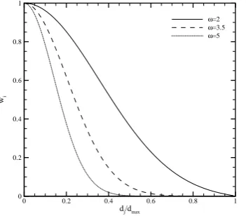
2.1 Eﬀect of parameter on the weighting function . . . 26

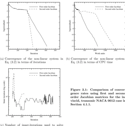
3.1 Comparison of convergence rates using ﬁrst and second order Jacobian

matrices . . . 49

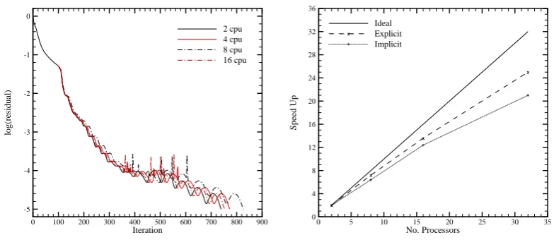
3.2 Parallel solver performance . . . 52

4.1 NACA 0012 aerofoil connectivities . . . 53

4.2 Transonic inviscid ﬂow for NACA 0012 aerofoil at Mach 0.8 and zero

degrees angle of attack using a quadratic polynomial reconstruction . . . 54

4.3 Supersonic inviscid ﬂow for NACA 0012 aerofoil at Mach 1.2 and 7.0

degrees angle of attack using a quadratic polynomial reconstruction . . . 55

4.4 Laminar ﬂow for NACA 0012 aerofoil at Mach 0.5, angle of attack 3.0

degrees and Reynolds number of 5000 using a quadratic polynomial

re-construction . . . 56

4.5 Laminar ﬂow over circular cylinder with Reynolds number of 40 . . . 58

4.6 Instantaneous contour plot of thexcomponent of velocity for the circular

cylinder, unsteady case with Reynolds number of 100 . . . 59

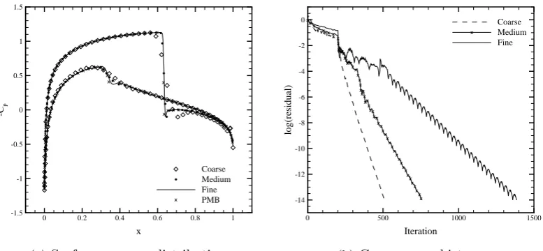
4.7 Pressure distributions and convergence histories for RAE 2822 aerofoil

case 9 . . . 60

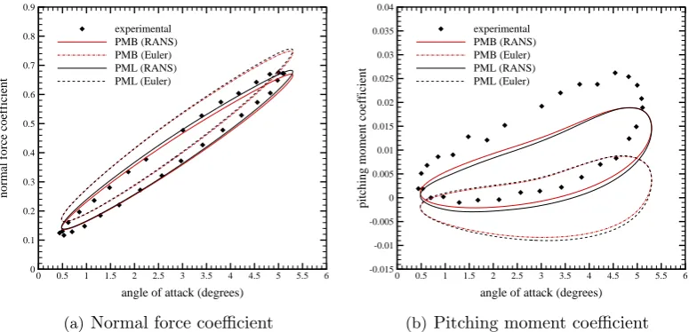
4.8 Normal force and pitching moment coeﬃcients for forced pitching motion

of AGARD CT1 test case . . . 61

4.9 Unsteady pressure distributions of AGARD CT1 test case . . . 61

4.10 Initial, steady state pressure contours and surface pressure distribution

for AGARD CT8 test case . . . 62

4.11 Comparison of real and imaginary parts of surface pressure distribution

for AGARD CT8 test case . . . 63

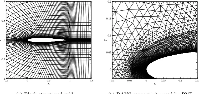
4.12 Stencils used by PML for three dimensional ﬂow solver validation . . . . 64

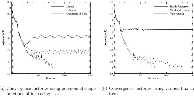
4.13 Comparison of convergence histories using shape function

(18)

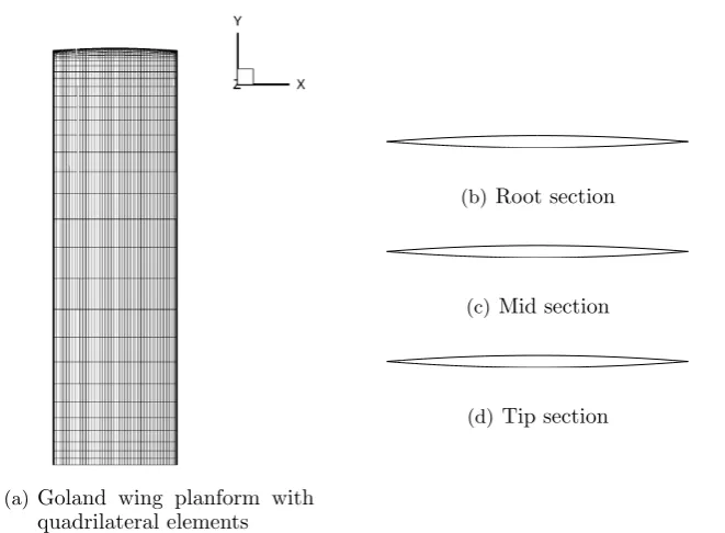
4.14 Goland wing planform with quadrilateral elements and cross sections . . 65

4.15 Pressure coeﬃcients for the Euler equations using quadrilateral and tri-angular elements at three freestream Mach numbers and two spanwise locations for the Goland wing . . . 66

4.16 MDO wing planform and cross sections . . . 67

4.17 Comparison of computed inviscid pressure coeﬃcients with PMB for the MDO wing test case . . . 67

4.18 ONERA M6 wing planform and cross sections . . . 68

4.19 Comparison of computed inviscid pressure coeﬃcients with PMB and experiment for the ONERA M6 wing test case . . . 69

5.1 Common neighbourhood concepts based on geometric criteria . . . 75

5.2 The partitioning process of the quadtree . . . 76

5.3 Candidate point search and stencil selections using nearest neighbour algorithms and anisotropic point distributions . . . 77

5.4 Required input for preprocessor . . . 79

5.5 Tests to determine if edges intersect using bounding boxes . . . 80

5.6 Boolean addition and subtraction of two overlapping cylinders . . . 81

5.7 Boundary intersection and reallocation diagrams for two bodies requiring Boolean addition . . . 82

5.8 Blanking point operations . . . 83

5.9 Situation with possible multiple ﬂaggings . . . 83

5.10 Comparison of results using classical nearest neighbour algorithm and presented stencil selection method for solution of the Blasius boundary layer on anisotropic point distributions . . . 85

5.11 Deﬁning the initial resolving vector and method of summation of over-lapping stencils . . . 86

5.12 Deﬁning coordinate system and parameters for the merit function . . . . 87

5.13 Results for biplane conﬁguration solving the Euler equations at Mach 0.5 and zero degrees angle of attack . . . 90

5.14 Results for biplane conﬁguration at inviscid ﬂow conditions Mach 0.755 and angle of attack 0.016 degrees . . . 91

5.15 Results for biplane configuration at inviscid flow conditions of Mach 0.755, angle of attack 0.016 degrees with a coarse, medium and fine upper aerofoil point distribution . . . 92

5.16 Results for the laminar biplane case at Mach 0.8, angle of attack 10 degrees and Reynolds number 500 . . . 93

(19)

5.18 Results for the RANS biplane case at Mach 0.7, angle of attack 1.49

degrees and Reynolds 9 million . . . 95

5.19 Input connectivities of the main body and control surface geometries . . 96

5.20 Close-up of boundary layer region at the intersection between the body and control surface . . . 97

5.21 Point distribution of the main body and control surface configuration at various angles of deflection, with pressure coefficient plots at turbulent flow conditions Mach 0.2, zero degrees angle of attack and Reynolds number 5 million . . . 98

5.22 Element bounding boxes in three-dimensions . . . 100

5.23 Method of redeﬁning the solid boundaries after intersection . . . 101

5.24 Blanking point operations in three-dimensions . . . 102

5.25 Determining the resolving vector using the principal axes of inertia . . . 103

5.26 Directions of anisotropy for stencils in three-dimensions . . . 104

5.27 Selection of points in basis for three-dimensional point distributions . . 105

5.28 Comparison of PML ﬂow solution and convergence history using initial grid connectivity and stencil selection methods on a Goland wing at freestream Mach number 0.9 and 0 degrees angle of attack . . . 106

5.29 Conﬁguration of the fuselage and wing input geometries, and new ele-ments that are created by the preprocessor as a result of the geometries intersecting for the DLR-F6 test case . . . 107

5.30 Surface pressure coeﬃcient plots for the DLR-F6 test case at Mach 0.8 and zero degrees angle of attack . . . 108

5.31 Resultant geometry of the OSF Case 2 when components are assembled 109 5.32 Surface pressure coeﬃcient plots for the OSF Case 1, at Mach 0.85 and 2.12 degrees angle of attack . . . 110

5.33 Pressure contours for OSF Case 2 at Mach 0.85, angle of attack 2.12 degrees . . . 111

6.1 Reconstruction of the stencils in regions with diﬀerent ﬂow types using the adaptive selection method and a new parameter . . . 114

6.2 Points moving in and out of the computational domain . . . 115

6.3 Point distributions at maximum control surface deﬂections . . . 116

6.4 Normal force and pitching moment coeﬃcients for unsteady forced con-trol surface deﬂection case . . . 117

(20)

6.6 View of stencils along the outer region of the input domain of the smaller

aerofoil, before and after the adaptive scheme has been applied, for the

laminar store release case . . . 120

6.7 Pressure coeﬃcient contours at two time steps for the Goland wing and store body case at inviscid ﬂow conditions Mach 0.5 and zero degrees angle of attack . . . 121

6.8 Transonic store release from OSF using prescribed motion . . . 122

6.9 Close up of missile, pylon and wing conﬁguration for the OSF store release test case . . . 123

7.1 Limitations in the summing of resolving vectors from two overlapping stencils . . . 127

7.2 Issues regarding point locations . . . 128

C.1 Ray-triangle intersection test . . . 148

C.2 Testing if the triangles lie in the same plane . . . 149

C.3 Tests to see if the triangles intersect using the intervals of the triangles on the line of intersection between the planes containing them . . . 150

C.4 Flag points belonging to two intersecting triangles . . . 152

C.5 Deﬁne the edges to be used in triangulation . . . 153

C.6 Candidate points per edge to be used in triangulation . . . 154

C.7 Remove non-conforming boundary points from candidate list . . . 155

C.8 Overlap of triangles belonging to same body . . . 156

C.9 Overlap of triangles belonging to opposite bodies . . . 157

(21)

List of Tables

1.1 Summary of classiﬁcation of meshless methods . . . 8

4.1 Convergence of lift, drag and moment coeﬃcients for inviscid transonic

case using linear and quadratic reconstructions using coarse, medium

and ﬁne point distributions . . . 54

4.2 Convergence of lift, drag and moment coeﬃcients for inviscid supersonic

case using linear and quadratic reconstructions using coarse, medium

and ﬁne point distributions . . . 55

4.3 Convergence of lift, drag and moment coeﬃcients for laminar case using

linear and quadratic reconstructions using coarse, medium and ﬁne point

distributions . . . 56

4.4 Angle of separation and drag coeﬃcients for laminar ﬂow over circular

cylinder with Reynolds number of 40 . . . 57

4.5 Comparisons of computed Strouhal number, mean pressure and mean

friction drag coeﬃcients . . . 59

4.6 Real and imaginary lift and moment coeﬃcients for AGARD CT8 test

case . . . 63

5.1 Timings for each stage of the preprocessor in seconds and as a percentage

of total computational time for the subsonic biplane case . . . 89

of total preprocessor time for the DLR-F6 case . . . 109

5.3 Components of the Open Source Fighter cases . . . 110

6.1 Timings for each stage of the laminar two-dimensional store case

prepro-cessor in seconds and as a percentage of total time . . . 118

6.2 Average timings for each stage of the preprocessor in seconds and as a

percentage of total time for the Goland wing and store body case. . . . 121

6.3 Size and quantity of additional components for the OSF store release case122

(22)

(23)

List of Symbols

a = speed of sound

A = Jacobian matrix (=∂R/∂p)

b, c, d = meshless shape function derivatives

c = chord length

Cd = drag coeﬃcient

Cf = skin friction coeﬃcient

Cl,Cm = coeﬃcients of lift and pitching moment

Cp = pressure coeﬃcient

cp,cv = coeﬃcients of speciﬁc heat

E = total energy

fi,fv = inviscid and viscous ﬂuxes in xdirection

gi,gv = inviscid and viscous ﬂuxes in y direction

hi,hv = inviscid and viscous ﬂuxes in zdirection

I = identity matrix

I = inertia tensor

k = reduced frequency

k = turbulence kinetic energy

L = reference length scale

m = pseudo-time level

m = order of polynomial

M_∞ = freestream Mach number

M = number of points on which local ﬂux depends

n = number of points in stencil

N = number of points in computational domain

N = shape function

n = unit normal vector

n = real-time level

P r,P rt = Prandtl number and turbulent Prandtl number

p = pressure

(24)

p = vector of base monomials

p = vector of primitive variables

q = heat ﬂux vector

R = residual vector

R = gas constant

Re = chord Reynolds number

t = real-time

T = temperature

t = unit tangential vector

u = vector of Cartesian velocity components

v = resolving vector

w = weighting function

w = vector of conservative variables

Greek Symbols

α = freestream angle of attack

α = pitch angle

α = vector of reconstructed polynomial coeﬃcients

β = control surface angle of deﬂection

γ = smallest distance in initial stencil

γ = ratio of speciﬁc heats

δ = boundary layer thickness

δij = Kronecker delta

ϵ = increment or tolerance

ζ = mapped coordinate system

η = spanwise location

η = basis vector

κ = thermal conductivity

µ,µt = dynamic viscosity and turbulent (eddy) viscosity

e

ν = intermediate variable of Spalart–Allmaras turbulence model

ξ = vector of basis coeﬃcients

ρ = density

τ = stress tensor

τ = pseudo-time

ϕ = ﬂow variables

ˆ

ϕ = meshless approximating function

ψ = ﬂux limiter

(25)

Subscripts

a = amplitude

e = eﬀective value

e = average of ﬂow variables within a set

h = halo value

i = interior point

i = star point

j = neighbouring point

L = left side of Riemann problem

o = orthogonal

R = right side of Riemann problem

t = turbulent

v = viscous model

0 = steady state solution, mean value or initial value

∞ = freestream value

Acronyms

6-DOF = six-degree of freedom

BILU = block incomplete lower-upper

CFD = computational ﬂuid dynamics

CFL = Courant-Friedrichs-Lewy

DLR = German Aerospace Center

GCR = generalised conjugate residual

MDO = multidisciplinary optimisation

MLS = moving least squares

MPI = message passing interface

MUSCL = monotonic upstream–centered scheme for conservation laws

NS = Navier–Stokes

ONERA = French Aerospace Lab

OSF = open source ﬁghter

PMB = parallel multiblock

PML = parallel meshless

POU = Partition of unity

RANS = Reynolds–averaged Navier–Stokes

SA = Spalart–Allmaras

(26)

(27)

Chapter 1 Introduction

The prediction of ﬂuid ﬂow involving moving aircraft components is a challenging prob-lem. An example of such an application is in store release, in which the store, a weapon

or countermeasure device, is released from the aircraft at high speed. Store

separa-tion analysis includes determining the trajectory during the initial stage of the release, and the identiﬁcation of safe separation zones to avoid mid-air collisions between the

store and the aircraft that released it. For this, important parameters such as the

miss distance, which is the smallest distance between any part of the store and the aircraft during the early part of the trajectory, are needed for all of the diﬀerent load

conﬁgurations and ﬂight conditions that are possible for the aircraft in question.

Originally, such parameters could only be determined with ﬂight tests, in which the stores were dropped from an aircraft at gradually increasing speeds until the store came

close to or actually hit the aircraft [1]. These tests were very dangerous for the test

pilots, and expensive in terms of time, implementation and the possible loss of aircraft. For many years wind tunnels were the only alternative; though with the recent advances

in computer hardware it is becoming more feasible to numerically compute the required

parameters using computational fluid dynamics (CFD). Such methods were first used to provide a solution for a store in an aircraft flow field in the 1970s [2, 3]. The continuing

development of computer resources and numerical algorithms, has meant that CFD has

matured to a state where it can work in conjunction with wind tunnel data and ﬂight tests in aerodynamic design.

The numerical methods employed in CFD require some discretisation of the

compu-tational domain: this is most commonly achieved through the use of a mesh, also called a grid. The mesh consists of a set of non-overlapping cells, which in some way conform

to the geometry of the problem, and ensure the conservation of the ﬂow variables. The

fluid flow over the geometry is simulated by transforming the governing equations of fluid dynamics into a discretised algebraic form, which is solved on the mesh to obtain

numerical (as opposed to analytical) solutions. For a store release case, these equations

(28)

on the store. This data is then used by a six-degree of freedom (6-DOF) module to

solve the rigid body equations of motion, and, thus, predict the store trajectory at each

time step. The computational domain for such simulations must include, at the very least, the aircraft from which the store is released and the store itself; hence, they form

what is called a multibody system. By classiﬁcation multibody systems may be static;

but the ﬂuid-structure interaction between the various bodies in the store release case inevitably leads to changing geometries during the time-dependent computation. This

means that there are elemental changes in the conﬁguration over time as the bodies

move relative to one another. The diﬃculties in handling such changes within a dis-cretised domain to account for this movement, is one of the important issues in the

simulation of this class of problem.

1.1 Moving-body problems in CFD

The most intuitive way to simulate moving-body problems is to generate a new grid at

each time step, with the bodies in the new locations as predicted by the calculations

made in the previous step. This means that each successive discretisation will require an interpolation of the ﬂow solutions between the grids, which leads to inaccuracies that

arise from the large number of interpolations that are needed. Also, as grid generation

can be a diﬃcult and time consuming process, remeshing the geometry after each time step is a very unattractive proposition. These disadvantages mean that researchers

have looked to alternative, more elaborate techniques.

One such technique is to deform the mesh to account for the body movement. In

this approach, the boundaries move according to the 6-DOF model after each time step, while the cells of the mesh expand and contract to accommodate the movement,

while keeping the connectivity unchanged between time steps [4–8]. This method is

relatively easy to implement into a CFD solver, and is adequate for motions that are simple. Problems arise when the bodies undergo large scale changes in their position,

meaning that the required mesh deformations are excessive: then the mesh quality

deteriorates and so must be reviewed during each iteration. Reference [9] presents a method in which the mesh is completely regenerated when it exhibits bad quality

measures. A local remeshing procedure is used in Ref. [10], in which a hole is cut in the

domain where the mesh quality has deteriorated; this region is then remeshed using an unstructured grid generator, thus, reducing where solution interpolation must occur.

Alternative methods arise by a decomposition of the domain into a set of simpler

subdomains. For example, it is convenient to generate independent grids around each

body separately, as subdomains, which can then be composited together in some way. If the grids meet at an interface, as in Fig.1.1(a), then they can slide past one

an-other to simulate the relative movement between the bodies. The meshes adjacent to

(29)

(a)Sliding mesh method (b) Overset grid method

Figure 1.1: Domain decomposition methods.

number of cell faces; hence, solutions must be passed through the interface by means

of an interpolation. This method requires that the motion of the bodies be known a-priori, and is restricted to movement along the interface. Applications, for which it has

been used with a great deal of success for time-dependent simulations, include

turbo-machinery [11], where non-matching and rotating cell faces are used for the simulation of the ﬂow between adjacent blade rows of engines; a study of noise generation from

propeller and propeller-wing conﬁgurations [12]; and the analysis of helicopter

aerody-namics [13], for which the unsteady ﬂow over a fuselage and rotor blades is computed for a helicopter in forward ﬂight. The restriction that the exact location of the bodies

must be known after each time step means, however, that there are limited

applica-tions to the sliding mesh approach; and it cannot be used to simulate many multibody problems with unknown geometry changes, such as those that occur in store release

cases.

A more ﬂexible method is obtained if instead of the domains meeting at the

inter-face, they are allowed to overlap, as shown in Fig.1.1(b). This means that the grids can move rigidly with their associated body components, and therefore, in theory, the

bodies can move in any direction relative to one another during the computation. This

grid movement can be performed without any deformation or remeshing, and communi-cation between the grids is achieved through data interpolation. This method is called

the overset grid method, though it is also commonly known as the Chimera method,

and was introduced in Ref. [14] by Steger et al. in 1983. The overset grid strategy not only has the beneﬁt of being able to simulate diﬃcult moving-body problems, but it can

also alleviate some of the diﬃculties in generating a full ﬁnite volume mesh, particularly

for multibody systems. The technique of overlapping grids to form the computational domain means that the engineer can construct meshes around bodies, or components

of bodies, independently, which is simpler and less time consuming than generating the

(30)

overset grid codes have been developed, such as those in Refs. [15–21]; these, and other

codes, have been used to solve moving-body problems in a wide range of applications

including helicopter flight [22, 23], tiltrotor flight [24], flow through a turbine [25] and store release [1, 26–32].

The use of overlapping grids means that a preprocessor stage is required to ﬁrst

cre-ate a computational domain on which the ﬂow solver can opercre-ate. This stage basically

consists of three steps: hole cutting, identiﬁcation of interpolation cells and identiﬁ-cation of corresponding donor cells. The hole cutting stage is necessary for regions of

grids that fall into solid bodies, or other non-ﬂow regions, when the overlap occurs:

these grid regions are removed from the computational domain. Interpolation cells are needed to establish the communication of the ﬂow solution between the grids; for each

grid, these cells will lie along hole boundaries and in other regions where interpolation boundaries are identiﬁed. Donor cells are then required from the other grids to create

stencils with the interpolation cells to make the inter-grid communication possible. In

steady state problems these procedures only need to be performed once, as the grid geometries remain invariant during the simulation. For problems with moving-bodies

the preprocessor stage has to be done after each time step, when the relative orientation

of the overset grids changes.

Unfortunately, these interpolation/donor cell identiﬁcation steps can be very diﬃ-cult. Ideally the donor and recipient cells will be of the same size in the overlap region;

if this is not the case, such as when one grid is highly reﬁned, this mismatch can cause

serious errors in the interpolation. This is because cells with lower resolution do not capture the ﬂow features that form in the areas of high resolution; and, consequently,

the magnitude of numerical error increases with the gradients of the ﬂow variables being

communicated [33]. This diﬃculty is often dealt with by the inclusion of another grid as a transition between the mismatching grids. This will increase the computational costs,

as a three-fold grid overlap in three-dimensions can be expensive, and additional

com-plexities in the above steps may arise. Also, the possibility of this happening at multiple geometric orientations during an unsteady, moving-body simulatation means that this

ﬁx is not ideal. There is also the problem of orphan points, which are interpolation

cells for which no valid interpolation is possible; this can happen, for example, if there is insuﬃcient overlap of the grids. Accuracy can also be compromised if an instance

occurs such that the donor elements in a grid are also interpolation locations. This communication of ﬂow data between grids is more problematic for viscous cases. These

diﬃculties mean that despite the successful applications of the Chimera method, there

are still limitations on its automatic use in moving-body problems when the bodies can move anywhere in the domain.

The above techniques all use the ﬁnite volume method, which uses cells to enforce

the conservation of mass, momentum and energy of the ﬂuid; as such, there is a clearly

(31)

if a cell comes into contact with another cell that has been used to discretise the ﬂow

around another body, then how to deal with the subsequent form of the cells, and

the ﬂuid inside each, is a major concern. This problem of the collision of such rigid structures invites the idea of breaking the restrictions that the cells impose. If only

the nodes were used, then there should be no problem in moving bodies relative to one

another: this is the basic idea behind the meshless method.

Meshless methods are characterised by the domain Ω requiring only a

distribu-tion of points for the soludistribu-tion of the equadistribu-tions. The ﬂow variables ϕ are each

represented by an approximating function ˆϕ, and are calculated by the use of

lo-cal clouds, or stencils. In the ﬁnite volume method, the surrounding cells

con-tribute to the stencil of each cell; in the meshless technique, each point i has a local

subdomain of neighbouring points Ωi that forms the stencil, as shown in Fig. 1.2.

O

0

O

1

O

2

O

3

O

4

O

5

O

1-½

O

2-½

O

3-½

O

5-½

O

4-½

Q

i

Q

i i

Figure 1.2: Form of a meshless domain.

As cells are not used at all, then some of

the diﬃculties associated with grid genera-tion can be avoided. In a similar manner

to the Chimera method, one can generate a

distribution of points around each body sep-arately, which adequately resolves the

geo-metric features, and the union of the point

distributions can then form the full compu-tational domain on which the solver directly

operates. Any incremental changes in the

geometry due to the bodies moving during a simulation will not require a complete regeneration of the points: only the local

sten-cils must change if the points within have moved. This is also beneﬁcial in the design

stage of aerospace vehicles: if only one component of the geometry needs to be changed, then only a regeneration of the points where the changes have occured is necessary.

As the separate distribution of points around each body is treated as an entity by the ﬂow solver, then, unlike with the Chimera method, there is no interpolation process

involved. This means that the rigorous and costly identiﬁcation of donor and

interpo-lation cells is not required, as the equations are solved directly in the regions where the point distributions overlap. It also means that there is no restriction on the resolution

of the various point distributions that overlap; and the bodies are, therefore, free to

move in any position relative to one another. This robustness is highly desirable with the large scale movements involved in some moving-body problems. The construction

of the stencils on the set of points may, however, be equally as diﬃcult as the

identiﬁ-cation of the interpolation stencils for the Chimera method. Research into algorithms for stencil selection are very important to determine if the method has the potential

to be a practical alternative to the Chimera method for problems involving multibody

(32)

1.2 Meshless methods

The Smoothed Particle Hydrodynamics (SPH) method [34, 35] is generally considered

to be the ﬁrst meshless method; and was introduced in 1977 to model astrophysical phenomena. Despite its initial success, it was only after the 1990s that SPH was applied

to a wider range of problems, such as impact, magnetohydrodynamics, heat conduction

and computational mechanics [36, 37]. In the SPH method an integral representation of a function, called a kernel approximation, is used to solve the governing partial

diﬀerential equations using a Lagrangian approach. The Reproducing Kernel Particle

Method [38] was proposed to correct the lack of consistency in SPH, by adding a correction function to the base kernel approximation, and so improving the accuracy.

Another class of meshless method, which was proposed later and has its origin in

data ﬁtting, can be obtained if one uses a moving least squares (MLS) interpolation to determine the approximation functions used for the governing equations. The Diﬀuse

Element Method [39] was the ﬁrst to use such a procedure; it was later reﬁned and

modiﬁed in the Element Free Galerkin (EFG) method [40]. EFG has become one of the most popular of the meshless methods, and has been applied to a wide range of

problems, such as fracture and crack propogation, wave propogation, acoustics and

ﬂuid ﬂow [41–44].

As pointed out in Ref. [45], each of these methods share many common features,

and, in most cases, MLS methods are identical to kernel methods. Any kernel method in

which the parent kernel is identical to the weight function of a MLS approximation, and is rendered consistent by the same basis, is identical. In other words, a discrete kernel

approximation which is consistent must be identical to the related MLS approximation. Underlying the two methods is the concept of the partition of unity (POU), which

provides a rational method for constructing localised approximations to global functions

with a greater degree of ﬂexibilty. The POU concept is used in the hp-cloud method [46] in conjunction with a MLS interpolation.

For all of these methods, the approximation function ˆϕwithin each subdomain Ωi,

for the pointi, can be expressed in the form

ˆ

ϕi(x) =

∑

j

Nj(x)ϕj (1.1)

where the sum is taken over each of the pointsj in the subdomain, andNj is the local

shape function. This form is also used in many ﬁnite element, including ﬁnite volume,

discretisations. The major diﬀerence, however, is that the local shape functions are

not reciprocal: this means that the shape function between a point and its neighbour within one stencil, is not the same as when the star is a point within the stencil of

the neighbouring point. Reciprocal shape functions mean that all interior ﬂuxes cancel

(33)

the domain boundaries. As a result, the meshless scheme cannot guarantee the

conser-vation of the ﬂow variables in the same way that conventional ﬁnite volume methods

can. The non-reciprocal shape functions make meshless calculations much slower than their mesh based counterparts; and, more importantly, the non-conservation may lead

to reduced accuracy. How much the lack of strict conservation will aﬀect the solution,

especially for turbulent ﬂows, is an area of ongoing research; though the issue has lead to doubts about the use of meshless methods in the scientiﬁc community.

As the various meshless methods are theoretically similar, a more useful way of

clas-sifying them is by their implementation. Generally, meshless methods can be classed as either Galerkin type methods or point collocation methods. Galerkin type methods

solve the weak form of the governing equations; formulations based on this form can

produce a stable set of algebraic equations, though integration procedures are required since the weak form satisﬁes the global integral form of the governing equations. This

integration is often done by the use of a background grid, which is used to create a

structure to deﬁne the quadrature points; consequently, such methods are not truly meshless. In practical terms though they can still be called meshless, as the grid

re-quired is very simple, and does not need to be compatible with the points in the domain.

The Meshless Local Petrov-Galerkin method [47], however, is based on the weak form, though it has a local nature in which the integral in the weak form is satisﬁed over

a local domain. As such, a global background integration is not required: only much simpler local integrals. This scheme has been used to solve the incompressible

Navier-Stokes equations in Ref. [48]. Point collocation methods, on the other hand, solve the

strong form of the governing equations on the set of points. Although obtaining the exact solution for a strong form system is often more diﬃcult and less stable, point

collocation methods are less complicated to implement, and are much less costly as

no background grid integration is required. It is for their speed and ﬂexibility that point collocation methods are generally preferred in CFD. The clouds of points are

used to solve the equations by ﬁrst discretising the derivatives of the partial diﬀerential

equation. This is done using an equivalent form of Eq. (1.1), which can be written

∂ϕˆi

∂x =

∑

j̸=i

b(i)j(ϕj−ϕi) (1.2)

where b(i)j is another local shape function for the subdomain i, associated with the

derivative of ˆϕi with respect to x; in this form, these shape functions must obey the

property _∑

j

b(i)j = 0 (1.3)

which is the equivalent of the partition of unity; and is called the partition of nullity for

(34)

Method System Approximation

Smoothed Particle Hydrodynamics Strong kernel

Reproducing Kernel Particle Method Strong or weak kernel

Diﬀuse Element Method Weak MLS

Element Free Galerkin Weak MLS

Meshless Local Petrov-Galerkin Weak MLS

Finite point method Strong MLS

hp-cloud Weak POU, MLS

Table 1.1: Summary of classiﬁcation of meshless methods by system as strong or weak, and approximation by kernel, moving least squares (MLS), or partition of unity (POU).

performing a local least squares approximation. Least squares methods already see wide

use in more traditional CFD methods, often as a means of reconstructing higher order variables in ﬁnite volume schemes [49]; meshless collocation methods are eﬀectively an

extension of this, in that we use least squares to directly compute the ﬂux derivatives.

The discretisation of the unknown function and its derivatives are deﬁned only by the position of the points, which means that domain overlap and multibody conﬁgurations

can be accommodated [46].

The ﬁrst use of point collocation meshless methods to solve problems in CFD was

by Batina [50], in which the Euler and Navier-Stokes equations were solved using an un-weighted least squares discretisation. This method was then used in Ref. [51] for simple

three-dimensional problems. This work can be seen as a precursor to the ﬁnite point

method developed by O˜nate et al., which was used for convection-diﬀusion problems

and compressible ﬂuid ﬂow [52, 53]. Improvements to the scheme include a suitable

mapping for increased stability [54], and an iterative QR decomposition method for

more robust shape function computation [55].

Most meshless methods used for CFD in the literature (including this work) use the ﬁnite point method or some variant. An example of such a variant is in the use of

a Taylor series representation of the approximating function, as opposed to a

polyno-mial representation. A Taylor series representation has been used in the Least-Squares Kinetic Upwind Method (LSKUM) [56, 57], which uses a meshless discretisation of the

Boltzmann equation, leading to an upwind scheme at the Euler level after taking

mo-ments. The stencils used are split stencils; and are selected according to the coordinate positions of the neighbouring points. The use of such stencils gives split ﬂux

deriva-tives and the upwind character to LSKUM. Praveen developed the Kinetic Meshless

Method [58], which diﬀers from LSKUM primarily in that a single stencil is used at each point; the upwinding is then introduced with the help of a modiﬁed least squares

approximation, called the dual least squares approximation. Katz and Jameson [59]

(35)

framework using grid connectivities. A multicloud algorithm, which enables simple

and automatic coarsening procedures to accelerate convergence for explicit schemes,

was also presented in Ref. [60]. A comparison is made between methods based on Taylor expansion, polynomial basis and radial basis function schemes in Ref. [61]. It

is shown that for transonic ﬂows with shocks, both the polynomial and Taylor series

representations performed well; however, there was a slight improvement in the lift and drag coeﬃcients when a polynomial representation is used.

A summary of the meshless methods described brieﬂy in this section is given in

Table 1.1; for a more detailed overview of the methods see Refs. [45, 62, 63].

1.3 Features of meshless methods in CFD

Another potential benefit of meshless methods is in the reduced effort required on behalf of the user to obtain CFD results. The lack of a mesh means that there is no predefined

connectivity; this provides ﬂexibility in adding or deleting points from a domain during

a computation for the purpose of automatic, adaptive reﬁnement. Such techniques are designed to capture physical features, for example shock waves, with high resolution. In

ﬁnite volume methods, this involves an often complicated procedure of splitting the cells in the areas of high gradient: the so called h-adaptivity. As meshless methods require

only a set of arbitrarily distributed points, an operation placing additional points in

these high gradient areas is a much simpler task. These regions are often identiﬁed by the use of some sort of error estimate at each point, which checks the resolution of the

solution. In a similar manner, one can easily take points away from regions where the

ﬂow is constant to save computational costs. The use of adaptive procedures means that reduced eﬀort is required in generating the points; and accurate computation of

the smaller scales of the ﬂow ﬁeld can be made, especially when we do not have a-priori

information concerning the solution.

Some examples in the literature include Ref. [64], which uses an error indicator to construct a list of points to be reﬁned; additional points are then inserted to surround

each of the points in the list. This is used in conjunction with an increased order of

polynomial in the approximating function, to form the full hp-adaptivity technique. Error estimates that use the diﬀerence in gradients at points and their neighbours

are also seen in Refs. [65] and [66]. The former adds the additional points using a

Voronoi/Delaunay technique; the latter adds points at the midpoint of the edge to be reﬁned. Instead of inserting and deleting points from the domain, one can alternatively

move the points around so that the errors in the estimators are minimised. This will

keep the computational costs constant between the reﬁnement stages, as the points

gradually approach the vicinity of the important ﬂow features. This movement is

generated using a spring analogy between the points in Ref. [67], while a reference

(36)

The ﬂexibility of meshless methods means that they can be used alongside other

CFD techniques. One such example is in the enforcement of boundary conditions for

embedded boundary systems: these systems arise in the use of non-conforming grids. The most common type of grid used is the Cartesian mesh due to ease of generation,

low storage requirements and low operation counts per cell compared to body-ﬁtted

grids; also, the lack of skewness and distortion of the cells often leads to improved convergence properties. The use of such grids means that the cells will often extend

through the surface of solid components. In ﬁnite volume boundary embedded schemes,

this problem can be overcome by the use of cut-cell methods. These methods can be very complicated, and lead to extremely small cells near the boundary, which may

not be ideal. Instead, one can use the meshless method to implement the boundary

conditions, which is much simpler. Reference [69] uses such a scheme to impose inviscid, slip boundary conditions on aerofoils: a simple ﬁnite diﬀerence numerical method is

used on the Cartesian nodes, and the surface points have meshless stencils formed from

the points making up the intersected cells. Additional points can be added in the sparse regions between the boundaries and Cartesian cells, formed as a result of the

intersection with the body geometry, to improve the stencil quality and resolution in

this region. Reference [70] presents a similar method to solve the Euler equations, but a ﬁnite volume method is used on the Cartesian mesh, and a simpler meshless approach

is employed in discretising the surface.

In the schemes outlined above, only a small fraction of the computational domain

is meshless. As meshless methods are typically more computationally expensive than

ﬁnite volume methods, these techniques exploit the advantages of the meshless method, but keep the costs low. To perform viscous calculations, however, it is not practical

to use solely unit aspect ratio Cartesian cells throughout the domain, as can be used for inviscid calculations. For this reason, the boundary embedded scheme has been

extended to other methods, using more of a hybrid of meshless, and ﬁnite diﬀerence

or ﬁnite volume techniques to solve the Navier-Stokes equations. The meshless clouds are preferred to resolve the viscous ﬂow features, so there are more meshless layers

of points than with the boundary embedded schemes. The Upwind Least Squares

based Finite Diﬀerence solver [71, 72] is one of the few meshless solvers to solve the Reynolds-Averaged Navier-Stokes (RANS) based turbulent ﬂow equations; this is done

in Ref. [73] using a hybrid of body-ﬁtted cells, Cartesian cells and points in which the

meshless computations take place. The body-ﬁtted cells have very high aspect ratio to capture the turbulent eﬀects, so are only a few layers thick, the Cartesian cells are

generated in the inviscid region, and the meshless points are located in the interface.

A preprocessor stage is needed to cut holes in the domain where grids overlap other grids and solid bodies; this preprocessor stage is also to classify each of the points, as

there are multiple solution methods involved. The points obtained from the body-ﬁtted

(37)

computing least squares derivatives on highly stretched point distributions; the points

from the Cartesian grid use a ﬁnite diﬀerence methodology to compute the derivatives

inexpensively; and a traditional, least squares meshless procedure is used on the points that fall between the body-ﬁtted and Cartesian point distributions.

Hybrid methods have also been used to solve three-dimensional ﬂow problems. A

Singular Value Decomposition Generalised Finite Diﬀerence scheme [74] solves viscous

problems using meshless clouds generated from the boundary surfaces in successive layers. The support nodes are selected simply by using the closest points contained

within the cells of the background Cartesian mesh, thus, the procedure can operate

across the diﬀerent grid schemes. This method has been used further in Ref. [75] for the problem of bodies undergoing large boundary movement, namely free falling and

rotating spheres: the Cartesian nodes remain stationary, while the meshless nodes move

with the motion of the bodies with which they are associated. A similar hybrid method was used in Ref. [76]; in this paper, blocks of Cartesian grids were generated, inside

which a box is cut to contain the geometry of the problem. The box is then ﬁlled with

meshless points, generated from an unstructured grid generator; and transition points, which form the vertices of the Cartesian cells next to the boundary of the meshless

region, provide the communication between the two regions. This solver format was used to study a time-dependent, inviscid store release case.

1.4 Stencil selection

Some of the solvers and methods described above may, on ﬁrst thought, seem

contra-dictory, since point distributions obtained from meshes are used to perform meshless computations. One can argue, however, that meshes have strict requirements regarding

the domain decomposition, which is lost when a solver uses only the point locations:

the concept of the cell and volume, the fundamental parts of a mesh, are ignored by a meshless solver (or the meshless part of a hybrid solver). The use of generated grids

for meshless computations means that there will be an adequate distribution of points

to resolve the geometric features that make up the problem. It also means that any type of grid can be used by the meshless solver, irrespective of its topology; and the

quality of the grids is not as strict as for the ﬁnite volume solvers, so requirements

such as positive volume, orthogonality, smoothness and skewness are not an issue. As mentioned, some of the diﬃculties associated with generation are alleviated further

when one generates points for a meshless computation around bodies, or components

of bodies, individually; the full point distribution is then obtained from combining these point distributions. Nevertheless, some eﬀort must still be expended in obtaining the

points; and, unless a generic, fully automatic point generation strategy is imposed, it

(38)

As well as obtaining the points for meshless methods, how the points form a

con-nectivity is also a concern. The stencils for each point used by the meshless solver take

the form of a set of neighbouring points on which the least squares approximations can take place. The full connectivity obtained in the meshing process has been used in

many papers concerning meshless solvers; the most common way is to simply use the

nodes from neighbouring cells in the grid connectivity to form the stencils. The test cases for which they are used are generally steady state problems for the purpose of

solver validation; the points are therefore stationary, and so there is no reason to change

the connectivity. Unsteady calculations with ﬁxed grid connectivities are performed in Ref. [77], in which an aerofoil is allowed to pitch and plunge within a ﬁxed domain. The

points change position to accommodate this movement, though the stencil

connectivi-ties do not change due to the mapping used during the point movement. The motion of the points during the simulation are very similar to those in the ﬁnite volume mesh

deformation method described earlier.

The main reason for the development of meshless methods, however, is for their greater ﬂexibility and freedom in the domain decomposition. This means that the points

that make up the domain would not start with a full connectivity; and so one would

need a method to establish the stencils for each point in a preprocessor stage. Therefore, the problem of stencil selection is unavoidable if meshless methods are to satisfy their

purpose for practical CFD calculations, otherwise the more established ﬁnite volume

methods could be used instead. As the choice of points in a stencil can seriously aﬀect accuracy and cost, this process is crucial if the method is to be competitive with ﬁnite

volume methods. Despite its importance, the problem of appropriate stencil selection

is, unfortunately, one that has not been addressed a great deal in the literature [78]. The construction of the local clouds is not trivial, and, although some papers have been

published on this subject, which are to be discussed, there does not appear to be a fully

robust, eﬃcient method for choosing the best stencils from any point distribution.

The points chosen for each stencil must be adequate for the least squares approxi-mations to take place; so there must be a minimum number of points that make up the

clouds to result in an overdetermined linear system. The points must not be arranged

to give a singular least squares matrix: so they cannot be collinear in two-dimensions, or coplanar in three-dimensions. One must also choose the points so that the functions

derived approximate the fluid flow accurately; for example, a boundary layer cannot be resolved accurately if a point that lies inside the highly viscous region uses flow values

from points deep within the inviscid region of the ﬂow in its stencil. Making sure that

this is not the case for random point distributions, particularly if they are not well spread or isotropic, is very diﬃcult.

Other issues include cost and automation. For any CFD problem in which the

bodies do not move, the stencil selection only has to be done once; as a result, there is

(39)

if the time taken to create the connectivity is less than the time needed to completely

mesh the problem. For use with time-dependent, moving-body problems, in which the

movement is not limited or known beforehand, the stencils will have to be selected after each time step when the points move relative to one another. Therefore, there can be no

user input for such cases; and as many stencil selection processes must take place within

the course of a computation, the selection must be done quickly and automatically.

A simple quadrant procedure in two-dimensions is described in Ref. [46], in which

the closest points in each quadrant around a given point are chosen for the stencil.

This is an improvement on a very simple nearest neighbour approach; and ensures that there are points in all directions around the point at which the ﬂow variables

are calculated, which means that the resultant stencils will be well-conditioned. A

Delaunay triangulation of local candidate points is presented in Ref. [79], in which the points that make up the triangles around the point (the ﬁrst layer) are retained for

the stencil. This method is eﬀectively a meshing procedure, with the stencils looking

similar to those of unstructured grids. Reference [80] uses a Gauss-Jordan pivoting method on a set of points to select the best points so that the shape functions satisfy

the Kronecker-delta property

bij =

{

1 ifi=j

0 ifi̸=j

This means that the consistency conditions and the partition of unity will be satis-ﬁed; though it means that the number of points in the stencil will always be equal to

the number of unknown coeﬃcients in the function to be approximated. Stencils are

selected with the property of positivity for the Laplace operator in Ref. [81]; positive stencils obey the POU of Eq. (1.3), and have a central local shape function coeﬃcient

b(i)i that is negative, while the neighbouring coeﬃcients are positive. This means that

the values ofb(i)j in Eq. (1.2) are all positive; and so a local minimum cannot decrease,

and a local maximum cannot increase. These stencils lead to an M-matrix structure,

which is beneﬁcial for linear solvers; however, there are necessary assumptions on the

point distributions that are made to ensure that positive stencils always exist. Geomet-rically, this condition is a cone criterion, in which points must be contained within a

cone with a deﬁned opening angle in whichever direction the cone points. If this is not

the case, then the points are deﬁned as not distributed nicely, and positive stencils are not guaranteed. A black box rule is given in Ref. [82] to select stencils of ﬁve points,

which are the nearest neighbours that satisfy a regularity restriction in the selecting

area. To do this, there are conditions which include restrictions on the collinearity of the points, and whether these points lie on a deﬁned quadratic curve.

The stencil selection methods described above can be classed as purely meshless

(40)

connec-tivity. Although this approach is ideal, the diﬃculties associated have lead to methods

that use some limited or initial connectivity as a guide to produce stencils: these

ap-proaches can be classed as semi-meshless. The hybrid schemes described in Section 1.3 use the body-ﬁtted and Cartesian mesh connectivities to form the meshless clouds in

the interface, so fall into this category. Similarly, a method in which clouds are formed

using the cell structures of grids is given in Ref. [83]. The grids are overlapped fully like in the Chimera method, and intersecting cells from each mesh form the stencils

that link them. The original connectivities are used throughout the rest of the domain

for the meshless solver. A set of lines eminating from boundary walls, deﬁned as a semi-mesh, is used in Ref. [84] as an aid in the stencil selection. These lines are used

to measure the orthongonality of the points; and a merit function is used that balances

the point distances and this orthogonality, to rank the neighbouring candidate points as the best to form the stencil.

As noted in Ref. [85], the type of stencils selected should depend on the equations

that are to be solved; and so a stencil selection algorithm should be developed, for a

speciﬁc set of equations, with this in mind. The reference, for example, uses the Laplace operator, which is isotropic, so the stencils should mimic this property; however, such

stencils could cause instabilities if a hyperbolic class of equation is to be solved, and

other stencil methods are preferable. The Navier-Stokes equations are not isotropic; and so the use of isotropic point distributions (or those with near unit aspect ratio)

are not practical to solve them. Instead, the point distributions are anisotropic in

regions near the boundary wall or in the wake, to capture high gradient ﬂows eﬃciently; consequently, a stencil selection algorithm that is to be used to solve the Navier-Stokes

equations should be developed with point distributions of this sort in mind. It means

that classic nearest neighbour algorithms (or variants of) are generally not sufficient for the task of selection over the entire domain. This poses difficulties regarding the efficient

selection of accurate, well-conditioned stencils on such point distributions, which this

thesis proposes to address.

1.5 Aim of work and outline of thesis

The aim of this work is the development of a CFD technique for the simulation of

moving-body ﬂows. The meshless method is used to solve the ﬂow equations globally

on a domain consisting of overlapping point distributions, which have been generated around each of the bodies independently. These point distributions are used to solve the

Navier-Stokes equations, so are anisotropic in form. Using overlapping point

distribu-tions, which are obtained from structured grids, means that there should be a suﬃcient number of points around the bodies to resolve the ﬂow; and moving-body cases can

be simulated by moving the input domains belonging to the bodies individually. The

(41)

initial connectivity of the individual point distributions as a guide, so the method can

be classiﬁed as semi-meshless; though the method is not a hybrid method, and putting

precedence on a single grid, or regions of several grids is not performed. For this work, we also avoid adding, moving or removing points from the domain to achieve the

sten-cils. The majority of the work presented is with regards to the development of a new

code at the University of Liverpool that has been written partly for the purpose of solving multibody problems, called Parallel MeshLess (PML) [86–91]. This thesis is

divided into two parts, for each of the main functions of the code: Part I consists of

Chapters 2, 3 and 4, and concerns the development of the meshless ﬂow solver; Part II consists of Chapters 5 and 6, and concerns the stencil selection method and application

to multibody systems.

Chapter 2 outlines the Navier-Stokes equations, which are the governing equations

of ﬂuid dynamics that are solved in this work. The spatial discretisation of these

equations using the meshless method is described: the method closely resembles the

ﬁnite point scheme mentioned earlier, in that the meshless approximation takes the form of a polynomial function, which is found using a weighted least squares method.

The calculation of the shape functions that are used to ﬁnd the ﬂux derivatives, and

the method of enforcement of the required boundary conditions is described.

Chapter 3 presents the temporal discretisation and the method of integration to

solve the diﬀerential equations provided by the meshless discretisation. The equations are solved implicitly using an iterative, preconditioned Krylov subspace method with

approximate, analytical Jacobian matrices. The parallelisation of the solver, so that

calculations can run on several computers, is also described.

Chapter 4 concerns validation to build conﬁdence in the PML ﬂow solver. Standard

inviscid, laminar and turbulent test cases for various steady and unsteady ﬂows are

computed in two and three-dimensions; and the results are compared with experimental data and other ﬁnite volume CFD solvers.

Chapter 5 presents the stencil selection method that is used to create the

connectiv-ity between the points that is used by the meshless ﬂow solver for multibody systems. The algorithm is described for two and three-dimensional cases; and is designed to

select robust stencils from any point distribution, regardless of their relative positions

and form. The novel concept of the resolving vector for accurate resolution of the ﬂow features is used for this purpose, and is applied to various steady state problems.

Chapter 6 uses the stencil selection method of Chapter 5, and is applied to

multi-body systems in which some of the bodies are moving in time-accurate computations. The additional complexities of simulating ﬂows with moving-bodies, such as point

ve-locities and solution interpolation, are described; and the method is tested ﬁnally by

(42)

(43)

Part I

(44)

(45)

Chapter 2 Spatial Discretisation

2.1 Navier-Stokes equations

The governing equations of ﬂuid dynamics considered are the Navier-Stokes equations.

These equations are derived from the principle of conservation of mass (continuity), momentum (Newton’s second law) and energy (the ﬁrst law of thermodynamics) of the

ﬂuid. For a Newtonian, isotropic ﬂuid with no heat sources, body forces or volumetric

heating, the Navier-Stokes equations can be written, for density ρ, components of

Cartesian velocityui and total energyE, in diﬀerential, conservative form as

∂ρ

∂t +

∂(ρui) ∂xi

= 0

∂(ρui)

∂t +

∂(ρuiuj) ∂xj

+ ∂p

∂xi

= ∂τij

∂xj ∂(ρE)

∂t +

∂ ∂xj

[uj(ρE+p)] =

∂ ∂xj

(uiτij−qj) (2.1)

wheret is the time, pis the pressure, τij is the viscous stress tensor and qi is the heat

ﬂux vector. Respecting Stokes’ hypothesis for an isotropic, Newtonian ﬂuid, the viscous

stress tensor can be written in component form as

τij =µ

[(

∂ui ∂xj

+∂uj

∂xi

)

−2

3δij

∂uk

∂xk

]

whereµis the coeﬃcient of viscosity (dynamic viscosity) andδij is the Kronecker delta

symbol. The heat ﬂuxes can be obtained using Fourier’s law of thermal conduction,

which states that

qi=−κ

∂T ∂xi

whereκ is the thermal conductivity andT is the temperature. To close this system of

On the development of a meshless method to study multibody systems using computational fluid dynamics