Analysis of stochastic fluid queues driven by local time processes

arXiv:0709.1456v1 [math.PR] 10 Sep 2007

Analysis of stochastic fluid queues driven by local

time processes

Takis Konstantopoulos∗ Andreas E. Kyprianou† Paavo Salminen‡0 Marina Sirvi¨o‡

July 12, 2018

Abstract

We consider a stochastic fluid queue served by a constant rate server and driven by a process which is the local time of a certain Markov process. Such a stochastic system can be used as a model in a priority service system, especially when the time scales involved are fast. The input (local time) in our model is always singular with respect to the Lebesgue measure which in many applications is “close” to reality. We first discuss how to rigorously construct the (necessarily) unique stationary version of the system under some natural stability conditions. We then consider the distribution of performance steady-state characteristics, namely, the buffer content, the idle period and the busy period. These derivations are much based on the fact that the inverse of the local time of a Markov process is a L´evy process (a subordinator) hence making the theory of L´evy processes applicable. Another important ingredient in our approach is the Palm calculus coming from the point process point of view.

Keywords: Local time, fluid queue, L´evy process, Skorokhod reflection, performance analysis, Palm calculus, inspection paradox.

AMS Classification: 60G10, 60G50, 60G51, 90B15.

1

Introduction

This paper extends the results of Mannersalo et al. [13] who introduced a fluid queue (or storage process) driven by the local time at zero of a reflected Brownian motion and served by a deterministic server with constant rate. The motivation provided in [13] is that the system provides a macroscopic view of a priority queue with two priority classes. Indeed, in such a system, the highest priority class (class 1) goes through as if the lowest one does not exist, whereas the lowest priority class (class 2) gets served whenever no item of the highest priority is present. In telecommunications terminology, class 2 only receives whatever bandwidth remains after class 1 served. As argued in [13], if the highest priority queue is, macroscopically, approximated by a reflected Brownian motion, the lowest priority

∗_{School of Mathematical and Computer Sciences, Heriot-Watt University, Edinburgh EH14 4AS, UK} †_{Department of Mathematical Sciences, The University of Bath, Bath BA2 7AY, UK}

‡_{Department of Mathematics, ˚Abo Akademi University, Turku, FIN-20500, Finland}

queue is driven by the cumulative idle time of the first one, which is approximated by the local time of the reflected Brownian motion at 0.

In view of Internet networking applications, such as the service provision amongst several classes of service (e.g. streaming video and expedited data), the fluid or macroscopic model is thus quite appropriate for obtaining a better picture of the situation and for performance analysis and design. From a mathematical point of view, the model is a rare example of a non-trivial fluid queue whose performance characteristics (such as steady-distribution) can be computed explicitly. If, in addition, we take into account the heavy-tailed nature of traffic on the Internet, it seems reasonable to consider a L´evy process as a model for class 1 queue. This provides motivation for studying a queue whose input is the local time of a reflected L´evy process.

More generally, let X be a Markov process and Lits local time at a specific point. The fluid queue driven by X refers to the stochastic system defined by

Qt=Q0+Lt−t+It, t≥0,

whereQt≥0 for all t≥0, andI is a non-decreasing process, starting from 0, such that

Z ∞

0

1

Thus,Qis obtained by Skorokhod reflection and I is necessarily given by

It=− inf

0≤s≤t[(Q0+Ls−s)∧0];

see [8]. By considering, instead of 0, an arbitrary initial time, we can define a proper stochastic dynamical system (see Appendix A for details) which, under natural conditions, admits a unique stationary version. To this we refer frequently throughout the paper.

We remark also that in Kozlova and Salminen [10] the situation in whichX is a general one-dimensional diffusion is analysed. Moreover, Sirvi¨o (n´ee Kozlova) [16] studies the case where L is constructed as the inverse of a general subordinator (without specialising the underlying processX).

This paper follows ideas which were developed in [16] in the context of reflection of the inverse of a subordinator. However, (1) it connects the abstract framework with the case where the subordinator is the local time of a reflected L´evy process (motivated by applications in priority processing systems) (2) it uses, as much as possible, a framework based on Palm probabilities (see, in particular, Section 4–Theorem 3 and Section 5–Lemma 2), and (3) explicitly discusses the possible types of sample path behaviour of the process of interest (Q); for illustration, see Figures 1, 2 and 3: Figure 1 concerns the case where Q

has continuous sample paths but with parts which are singular with respect to the Lebesgue measure. Figure 2 concerns the case whereQhas paths with isolated discontinuities (positive jumps) and linear decrease between them. Figure 3 concerns the case whereQhas absolutely continuous paths. The cases are exhaustive. Despite the wide variety of sample paths (depending on the type of underlying L´evy process Y), the mathematical framework and formulae derived have a uniform appearance.

version of X. In Section 4 we derive the stationary distribution of the buffer content and present a number of examples. In Section 5 we examine the idle and busy periods, and, in particular, characterise the distributions of their starting and ending times. The analysis is carried out first under the condition that the time at which the system is observed is a typical point of and idle or a busy period. Finally, the distributions of typical idle and busy periods are derived.

2

The background Markov process and its local time

We first construct the underlying Markov process X which models the highest priority class. This process will be taken to be the stationary reflection of a spectrally one-sided L´evy process

Y = (Yt, t∈R)

with two-sided time and Y0 = 0 (see Appendix B). A L´evy process is called spectrally

negative if its L´evy measure Π satisfies

Π((−∞,0))>0 and Π((0,+∞)) = 0,

and spectrally positive if

Π((−∞,0)) = 0 and Π((0,+∞))>0.

Clearly, ifY is spectrally positive then−Y is spectrally negative, and vice versa. To avoid trivialities we shall throughout assume that

|Y|does not have monotone paths

which rules out the cases that Y is an increasing or decreasing subordinator.

We also discuss the characteristics of its local time at 0. Appendix A summarises the notation and results on the Skorokhod reflection problem and its stationary solution. Ap-pendix B summarises some facts on L´evy processes with one sided jumps indexed byR_{. We}

will throughout denote byP a probability measure which is invariant under time shifts, and by Px the conditional probability measure whenX0 =x. We define the Laplace exponent

of a spectrally one-sided L´evy process as a function ψY :R+→Rgiven for θ≥0 by

ψY(θ) :=

(

logEeθ(Yt+1−Yt)_{, if Y is spectrally negative ,}

logEe−θ(Yt+1−Yt)_{, if Y is spectrally positive.}

Thus we insist that ψY be defined onR+, and define its right inverse

ΦY(q) := sup{θ≥0 : ψY(θ) =q}, q≥0. (1)

We use also the notation

Yt:= sup 0≤s≤t

Ys and Yt:= inf

0≤s≤tYs, t≥0,

and recall the duality lemma for L´evy processes (see, e.g., Bertoin [2, p. 45]):

{Yt−Y(t−s)− : 0≤s≤t}

d

where= means equality in distribution. Hence,d sup

0≤s≤t

Yt−Y(t−s)−=d Yt,

which is equivalent with

Yt−Yt d

=Yt. (3)

In this paper, we will mainly study the L´evy process Y with the time parameter taking values in the whole of R _{(see Appendix B). The Skorokhod reflection mapping associated}

with{Yt : t∈R} is defined (see Lemma 8 in Appendix A) via

Xt:=Rte Y := sup

−∞<s≤t

(Yt−Ys), t∈R.

In the remaining of this section we give conditions for the existence of the stationary process1 e

RY = (Rte Y, t∈R_{), compute its marginal distribution, and define the local time process L}

of ReY at 0 which will be used for the construction of the fluid queue. A few words about the definition of L are in order. We adopt the point of view theL is a stationary random measure on (R_,B_{), i.e.}

L(s, s+t] =L(0, t]◦θs, t≥0, s∈R,

where θs is the shift on the canonical space (see Appendix B), which regenerates together

with X at each pointt at which Xt= 0. It is known that L is a.s. continuous if and only

if the point x = 0 is regular for the closed interval (−∞,0] for the process X, and this is equivalent to inf{t >0 : Yt≤0}= 0,P0-a.s. Furthermore,Lis a.s. absolutely continuous if

and only if, in addition to the above, the pointx= 0 is irregular for the open interval (0,∞) for the process X, and this is equivalent to inf{t > 0 : Yt > 0} > 0, P0-a.s. If L is a.s.

continuous then it is not difficult to attach a physical meaning to it as a cumulative input process to a secondary queue. For mathematical completeness, we shall also consider the case whereLis a.s. discontinuous, in which case it can be shown to have a discrete support. In the continuous case, L can be defined uniquely module a multiplicative constant. We shall make the normalization precise later. In the discontinuous case, there is more freedom; however, insisting that its inverse be a subordinator, we are left with only one choice. The discontinuous case appears only once below and the construction of Lis discussed there. In all cases, the support of the measure Lis the closure of the set {t∈R_{:Xt= 0}.}

Associated to the measure (L(B), B∈B_{) we can define a cumulative local time process,}

denoted (abusing notation), by the same letter, and given by:

Lt:=

(

L(0, t], t≥0,

−L(t,0], t <0.

The right-continuous inverse process is

L−_x1 := (

inf{t >0 : L(0, t]> x}, x≥0

sup{t <0 : L(t,0]< x}, x <0. (4)

In case L is P-a.s. continuous, the process (L−1

x , x ∈ R) has, under P0, independent

in-crements and a.s. increasing paths (i.e. it is a, possibly killed, subordinator). This is an additional requirement that needs to be imposed when Lis not P-a.s. continuous.

Throughout the paper, we denote by Px the probability P, conditional onX0 =x. 1_{That this process is Markov is easy to see due to the independence of the increments of}

2.1 Stationary reflection of a spectrally negative L´evy process

Suppose that the processY is a spectrally negative L´evy process with non-monotone paths; see expression (53).

Proposition 1. Let Y ={Yt : t∈R} be a spectrally negative L´evy process with two-sided

time. Assume that its Laplace exponentψY(θ) = logEeθY1,θ >0, is such that ψ_Y′ (0+)<0.

Then

X ={Xt:=Rte Y : t∈R}

is the unique stationary solution of SDS (the Skorokhod dynamical system, see Appendix A) driven by Y. The marginal distribution of X is exponential with mean 1/ΦY(0).

Proof. SinceE[Yt+1−Yt] =ψ′Y(0+)<0, existence and uniqueness of the stationary solution

is guaranteed by Corollary 2 of Appendix A. That ΦY(0)>0 is a direct consequence of the

definition of ΦY (see (1)). To derive the marginal distribution ofX consider for β ≥0

E[e−βX0_{] = lim}

t→∞E0[e

−β(Yt−Yt)_{] = lim}

t→∞E0[e −βYt_]

SinceY is spectrally negative its over all supremum, sup_s≥0Ys,is exponentially distributed

with mean 1/ΦY(0) (see, e.g., Bertoin [2, p. 190] p. 190 or Kyprianou [11, p. 85]).

In view of Proposition 1, we assume that

ψ_Y′ (0+)∈[−∞,0),

which is equivalent to

ΦY(0)>0.

It is easily seen that, for a non-monotone spectrally negativeY, a necessary and sufficient condition for continuity of L is that Y has unbounded variation paths. This is further equivalent to: σ >0 or R₋0₁|y|Π(dy) =∞.

In the alternative case, when the paths of Y are of bounded variation, the number of visits of Y to its running infimum forms a discrete set. So n(s, t] := P_u∈R

1

finite for all −∞< s < t <∞. Let nt:=n(0, t] ift≥0, andnt:=−n(t,0] if t <0, and let

(e_j, j ∈Z) be a collection of i.i.d. exponentials with mean 1, independent of Y. We adopt the following construction forL.

L(s, t] = X

ns<i≤nt

e_i, −∞< s≤t <∞.

In both cases, the process (L−_x1, x∈R_{) is a subordinator underP0, withL}−1

0 = 0,P0-a.s.

IfLis continuous, this property is immediate from the definition ofL. IfLis discontinuous,

L−1 has independent increments due to our choice of the exponential jumps of L. Since

ψ′

Y(0+)< 0, we have Yt → ∓∞, as t → ±∞, P-a.s., and this implies that Lt → ±∞, as

t→ ±∞,P-a.s. Thus, it is not possible for L−1

x to explode for finitex.

Regardless of the continuity of the paths of L, we always have the following:

Proposition 2. Let Y and X be as in Proposition 1 and L the local time at 0 of X.Then

the local time L can be normalized to satisfy

E0e−qL −1

and, moreover,

E0L−x1=x/ΦY(0), x ∈R, ELt=tΦY(0), t∈R. (6)

Proof. For the Laplace exponent of L−_x1 in (5), we refer to Bingham [3, p. 731] (a result due to Fristedt [5]) and Kyprianou [11] and Kyprianou and Palmowski [12]: The “ladder process” (L−_x1, X_L−1

x ), x≥0) is a L´evy process with values in

R2

+ and Laplace exponent

b

κ(α, β) = logE0e

−αL−1

1 −βXL−₁1₌ α−ψY(β)

ΦY(α)−β

obtained by Wiener-Hopf factorisation for a spectrally negative process; see Bertoin [2, p. 191, Thm. 4]. Setting β = 0 we obtain E0[e−αL

−1

1 ] =e−α/ΦY(α)_{, as claimed. From this, we}

obtain E0L−x1 = x/ΦY(0), by differentiation. Using the strong law of large numbers, we

have limx→∞L−x1/x= 1/ΦY(0),P0-a.s., and, given that (L−x1, x >0) is the right-continuous

inverse function of (Lt, t > 0)–see (4), we have limt→∞Lt/t = ΦY(0), P0-a.s., and P-a.s.

Since L is a stationary random measure, we have ELt =C t for some constant C. Hence,

we immediately have thatC = ΦY(0), and this proves (6).

We shall later need theP-distribution of the random variable

D:= inf{t >0 : Xt= 0}. (7)

SinceX0 is exponential with rate ΦY(0), we haveP(X0 >0) = 1. So if 0≤t < D, we have

Xt=X0+Yt,P-a.s. Therefore

D= inf{t >0 : Yt<−X0}, P −a.s.

Let

τ−x := inf{t >0 :Yt<−x}.

Therefore,

E[e−θD] =

Z ∞

0

P(X0∈dx)E[e−θτ−x]

=

Z ∞

0

ΦY(0)e−ΦY(0)x

Z(θ)(x)− θ

ΦY(θ)

W(θ)(x)

dx

= ΦY(0)

ψY(ΦY(0))ΦY(θ)−θΦY(0)

ΦY(θ) ΦY(0) [ψY(ΦY(0))−θ]

= ΦY(0) ΦY(θ)

, (8)

where the overshoot formula (61) given in the Appendix B (see also Bingham [3, p. 732]) and the Laplace transforms (56), (57), for the scale functionsW(θ)_,Z(θ)_{, were used.}

2.2 Stationary reflection of a spectrally positive L´evy process

We can repeat the construction in the subsection above for a spectrally positive L´evy process

Proposition 3. Let Y ={Yt : t∈ R} be a spectrally positive L´evy process with two sided

time and Laplace exponent ψY. Assume that its Laplace exponent ψY(θ) = logEe−θY1 is

such that ψ′_Y(0+) > 0. Then the process {Xt := Rte Y : t ∈ R} is the unique stationary

solution to the SDS driven by Y. The stationary distribution of X is given for β≥0 by

E[e−βX0_{] = lim}

t→∞E0[e

−β(Yt−Yt)] = lim

t→∞E0[e −βYt)_]

=ψ_Y′ (0+) β

ψY(β)

. (9)

Proof. Notice that in this case, by the assumption onψY,

E[Yt+1−Yt] =−ψY′ (0+)<0,

and, hence,Y drifts to−∞.Let Z :=−Y. Clearly, Z is spectrally negative,

Xt=Yt−Yt=Zt−Zt,

andZ drifts to +∞.The classical result due to Zolotarev [18] (see also Bingham [3] Propo-sition 5 p. 725) says that the stationary distribution of X is as given in (9).

We shall therefore assume that

ψ′_Y(0+)∈(0,∞).

Hence ΦY =ψ−_Y1 and so

Φ′_Y(0+) = 1/ψ′_Y(0+)∈(0,∞).

It is easily seen that, starting from 0, the process Y hits (−∞,0] immediately, P-a.s., and this ensures continuity of the local time L. Moreover, we may and do normalize L so that

L(s, t] =− inf

s<u≤tY(s, u]. (10)

The continuity of Limplies that

{L−_x1 : x≥0}={τ−x : x≥0}, (11)

where τ−x := inf{t > 0 : Yt < −x} = inf{t > 0 : Zt > x}. Note that (L−x1, x ∈ R) is

a subordinator under P0, with L−01 = 0, P0-a.s. Furthermore, since Yt drifts to ∓∞ as

t→ ±∞,L−1 is proper (not killed).

Let us briefly comment on the special case where, starting from X0 = 0, the interval

(0,∞) will be first visited by X at an a.s. positive time. It is known [2, Ch. 7] that this occurs if and only ifY has bounded variation, i.e.

Y(s, t] =dY(t−s) +

Z

(s,t] Z

(0,∞)

y η(du, dy), (12)

wheredY is the drift, andR₀1y Π(dy)<∞. Since we exclude the case whereY is monotone,

we must have dY <0. In that case, with (10) as the definition ofL, it is known that for all

s≤t,

L(s, t] =|dY|

Z t

s

1

Proposition 4. Let Y be as in Proposition 3 and L the local time at 0 of X. Then

E0[e−qL −1

x _{] =e}−ΦY(q)x_{, q ≥0. (14)}

Moreover,

E0L−x1 =xΦ′Y(0+), x≥0, ELt=t ψ′Y(0+), t≥0. (15)

Proof. Formula (14) follows from (11) and the well known characterisation of the distribution of the first hitting timeτ_x+,see, e.g., Bingham [3] p. 720. By differentiating (14), we obtain the first part of (15), and using an ergodic argument–as in the proof of the second part of (6)–we obtain the second part of (15).

We now compute the P-distribution of D= inf{t >0 : Xt= 0}, by arguing as earlier:

we haveD= inf{t >0 :−Yt> X0}, and, since−Y is spectrally negative, we use the hitting

time formula (60) of Appendix B to obtain

E[e−θD] =E[e−ΦY(θ)X0_{] =ψ}′

Y(0+)

ΦY(θ)

ψY(ΦY(θ))

=ψ_Y′ (0+) ΦY(θ)

θ , (16)

where we also used (9) and the fact that ΦY◦ψY is the identity.

3

Construction of (the stationary version of ) the fluid queue

with local time input

We wish to construct a fluid queue driven by

b

L(s, t] =L(s, t]−(t−s),

where L is the local time at zero of the Markov processX. The process X is a stationary Markov process which is the reflection of a spectrally negative (Section 2.1) or a spectrally positive (Section 2.2) L´evy process. In either case, L is a stationary random measure with rate (see (6) and (15))

µ=EL(s, s+ 1] = (

ΦY(0), if Y is spectrally negative

ψ′_Y(0+), if Y is spectrally positive . (17)

The fluid queue started from levelx at time 0 is, as explained in Appendix A, the process

(R0,tLb(x), t≥0).

From Corollary 2 in Appendix A we immediately have:

Theorem 1. If µ < 1 there is a unique stationary version of the fluid queue driven by Lb

and is given by

Qt=Rte Lb = sup

−∞<u≤t

(Lbt−Lbu), t∈R. (18)

Thus, the following assumptions will be made throughout the paper:

[A1] µ <1

Assumption [A1] is so that we can construct a stationary version of Q (as in Theorem 1). If Y is spectrally positive and of bounded variation non-monotone paths then its drift dY

must be negative. If, however, |dY| ≤1 then–see (13)–L(s, t]≤t−sfor all s < tand so Q

will be identically equal to 0.

Physically, we think ofQa stationary fluid queue whose cumulative input between times

sand tisL(s, t] and whose maximum potential output ist−s. Unlike X, the processQ is

not Markovian. However, since Qhas been built on the probability space supporting X, it makes sense to consider, for eachx≥0, the probability measurePx defined asP conditional

on {X0 =x}.

Since L is a random measure allows us to consider the Palm distribution with respect to it, namely the probability measure defined by

PL(A) =µ−1E

Z

(0,1]

1

Since PL is also given as the value of the Radon-Nikod´ym derivative

PL(A) =µ−1

E

1

dt

_t=0

it follows that PL expresses conditioning with respect to the event that t= 0 is a point of

increase of L. But L is the local time of X at zero. Therefore, the support ofL is the set of zeros ofX. We thus have

Theorem 2. The Palm measure PL coincides with P0.

This observation allows us to use the formulae of Appendix A involving Palm probabil-ities.

4

Stationary distribution of the fluid queue

We are interested in computingP(Qt ∈ ·), a probability measure which is the same for all

t. We will use three properties of L. First, duality, i.e. that Y has the same distribution when time is reversed, see (2), implies that

(L(0, t], t≥0)= (d L[t,0), t≤0), underP and underPL.

Second, the process

L−_x1= inf{t≥0 :L(0, t]> x}, x≥0

is a subordinator under P0. Third, the Palm measurePL coincides withP0.

Recall thatψY(θ) has been defined as logEeθ(Yt+1−Yt)whenY is spectrally negative and

as logEe−θ(Yt+1−Yt) _{when Y is spectrally positive. The reason is that it is customary to}

have θ≥0 in both cases. Recall also that ΦY(q) = sup{θ≥0 :ψY(θ) =q}. The stationary

distribution of Q will be expressed in terms of ψY. For earlier works on this problem, we

refer to [15] for diffusion local times and [16] for the inverse of a general subordinator. The present formulation in Theorem 3 is in particular tailored for the local time ofX.The proof makes use of the Palm probability which is a new ingredient.

Lemma 1. Let R_:=R_{∪ {+∞,−∞}, If h:}R_→R _{is right-continuous and non-decreasing}

then h−1_{(x) := inf{t: h(t) > x}, x∈R, is right-continuous non-decreasing, h}−1 _{:R→ R,}

and, for all t∈R_,

h−1(h(t−)−)≤h−1(h(t)−) ≤t≤h−1(h(t−))≤h−1(h(t)). (19)

Furthermore, (h−1)−1 =h.

Theorem 3. (i) IfXis the reflection of a spectrally negative L´evy processY withψ′

Y(0+)<

0, ψY(1)>0 then

P0(Q0 > a) =e−ψY(1)a, P(Q0 > a) = ΦY(0)e−ψY(1)a, a≥0.

(ii) If X is the reflection of a spectrally positive L´evy process Y with 0< ψ′

Y(0+)<1 and

dY <−1 in the case of bounded variation, then

P0(Q0 > a) =e−θ ∗_a

, P(Q0 > a) =ψY′ (0+)e−θ ∗_a

, a≥0,

where θ∗>0 is defined by ψY(θ∗) =θ∗.

Proof. By the construction of Qand duality, we have P(Q0 ≤a) =P(supu≥0(Lu−u)≤a).

At this point we note that our assumptions imply that the process{Lt−t:t≥0}does not

have monotone paths. The event {sup_t≥0(Lt−t)≤a} can be expressed in terms ofL−1:

{sup

t≥0

(Lt−t)≤a}={sup x≥0

(x−L−_x1)≤a}.

To justify this (recall that in case (i) L is not necessarily continuous), we first assume that

Lt≤t+afor all t≥0. HenceLL−1

x ≤L

−1

x +afor all x≥0. Since (Lemma 1)

L_L−1

x ≥x, x≥0.

we have x ≤ L−1

x +a for all x ≥ 0 and thus supx≥0(x −L−x1) ≤ a. Assume next that

x−L−1

x ≤ 0 for all x ≥ 0. Then limε↓0L−x−1ε = L−x−1 ≥ x−a for all x ≥ 0. Therefore,

L−_(L1

t)−≥Lt−afor allt≥0. Since (by Lemma 1 again) L−_(L1

t)− ≤t, t≥0,

we obtain L−_(L1

t)− ≥t−a for allt≥0 and this gives supt≥0(Lt−t) ≤a. We first compute

theP0-distribution ofQ0:

P0(Q0> a) =P0(sup x≥0

(x−L−_x1)> a), a≥0.

Under P0, the process

{Λx :=x−Lx−1 : x≥0}, (20)

is a spectrally negative L´evy process with bounded variation paths. Letting

σa:= inf{x: Λx> a},

and applying Lemma 10 of Appendix B, we have

P0(Q0> a) =P0(σa<∞) = lim q↓0E0

e−qσa_{= lim}

q↓0 e

The function ΦΛ(q) is given by

ΦΛ(q) = sup{θ≥0 :ψΛ(θ) =q}, q≥0

(see (55)), where

ψΛ(θ) = logE0eθΛ1=θ+ logE0e−θL −1 1 .

If Y is spectrally negative, then we use Proposition 2 for an expression for logE0e−θL −1 1 . IfY is spectrally positive we use Proposition 4. We obtain:

ψΛ(θ) = (

θ−_Φθ

Y(θ), if Y is spectrally negative, θ−ΦY(θ), if Y is spectrally positive.

(22)

In both cases, Q0 is exponential underP0. with parameter ΦΛ(0), which has different value

in each case. Letµbe the rate of L (see (17)). Using equation (51), we have

P(Q0 > a) =µPL(Q0 > a) =µP0(Q0 > a) =µe−ΦΛ(0)a, a≥0. (23)

The proof will be complete, if we show that

ΦΛ(0) = (

ψY(1), if Y is spectrally negative,

θ∗, if Y is spectrally positive.

Note that ΦΛ(0) is the positive solution of ψΛ(θ) = 0. If Y is spectrally negative, we see,

from the first of (22), thatψΛ(θ) = 0 iff ΦY(θ) = 1 and, by the definition of ΦY, the latter

is true iff θ = ψY(1). Thus, ΦΛ(0) = ψY(1). If Y is spectrally positive, ψΛ(θ) = 0 iff

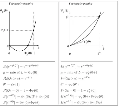
Table showing the basic characteristics of the system in both cases Φ (0) Y ψ Y(θ) 000 111 000 111 0 0 0 0 0 0 0 0 0 0 0 0 0 0 0 1 1 1 1 1 1 1 1 1 1 1 1 1 1 1

Y spectrally negative

θ 0 1 0 ψ Y(1)

E0[e−qL −1

x _{] =e}−xq/ΦY(q) µ= rate ofL = ΦY(0)

P0(Q0 > a) =e−θ ∗_a

θ∗_=ψ

Y(1)

P(Q0 = 0) = 1−ΦY(0)

E[e−θX0_{] = Φ}

Y(0)/(θ+ ΦY(0))

E[e−θD] = ΦY(0)/ΦY(θ)

ψ Y(θ) θ∗ θ∗ 0 0 1 1 00000000000000000000000 11111111111111111111111 0 0 0 0 0 0 0 0 0 0 0 0 0 1 1 1 1 1 1 1 1 1 1 1 1 1 0 0 0 1 1 1 Y spectrally positive

θ 0

0

ψ Y(0)

E0[e−qL −1

x _{] =e}−xΦY(q) µ= rate of L=ψ′

Y(0+)

P0(Q0 > a) =e−θ ∗_a

θ∗=ψY(θ∗)

P(Q0= 0) = 1−ψ′Y(0)

E[e−θX0_{] =ψ}′

Y(0+)θ/ψY(θ)

E[e−θD_{] =ψ}′

Y(0+) ΦY(θ)/θ

4.1 Example 1: Fluid queue driven by the local time of a reflected

Brow-nian motion

ConsiderY to be a Brownian motion with drift (see also [15], [13], [10]):

Yt:=σBt−µt, t∈R,

where σ >0, µ > 0. Here B = (Bt, t∈ R) is a standard Brownian motion with two-sided

time. In other words, (Bt, t≥0), (B−t, t≥0) are independent standard Brownian motions

with B0 = 0 (although specification of B0 does not affect the results below). The L´evy

measure here is 0. ConsiderY as in Section 2.2 and let

ψY(θ) = logE[e−θY1] =

1 2σ

2_θ2_{+µθ, θ >0.}

Define

Xt=Rte Y = sup

−∞<s≤t

σ(Bt−Bs)−µ(t−s), t∈R.

Lemma 3 gives the distribution ofX0 under P:

Ee−βX0 _=ψ′

Y(0+)

β ψY(β)

= ₁ µ

2σ2β+µ

i.e. exponential with rate 2µ/σ2. Let L be the local time at zero of X. The rate of L–see (17)–is ψ′

Y(0+) =µ. Assumeµ <1. LetLb(s, t] =L(s, t]−(t−s) and letQbe defined by

Qt=Rte L,b t∈R.

Theorem 3 gives the distribution of Q0 under P:

P(Q0 > a) =ψY′ (0+)e−θ ∗_a

=µe−2(1−µ)a/σ2, a≥0.

Here, θ∗ _{was found from ψ}

Y(θ∗) = θ∗. Thus Q0 is a mixture of an exponential with rate

2(1−µ)/σ2 and the constant 0 which is assumed with probabilityµ.

4.2 Example 2: fluid queue driven by the local time of a compound

Pois-son process with drift

Suppose that, forα >0,

Yt=St−αt, t∈R,

where S is a compound Poisson process with only positive jumps, jump rate λ and jump size distribution F. For simplicity, we take F to be exponential with rate δ > 0, i.e.

F(dx) =δe−δx_{dx. Then}

ψY(θ) = logEe−θ(Yt+1−Yt)=αθ−λ

Z

[0,∞)

(1−e−θx)F(dx) =αθ− λθ

δ+θ, θ >0.

The assumption 0< ψ′(0+)<1 implies that 1 +λ/δ > α > λ/δ. Moreover, the assumption

|dY|>1 implies additionally that α >1. We can define the background stationary Markov

process by

Xt=RetY = sup

−∞<s≤t

(St−Ss−α(t−s)), t∈R.

We have

Ee−βX0 ₌ α−λm

α−λR_[0,∞)1−e_β−βxF(dx).

Unlike the previous example, here P(X0 = 0) = limβ↑∞Ee−βX0 =α−λ/δ >0. The local timeL of X at 0 has rate

µ=ψ_Y′ (0+) =α−λ/δ.

The assumptions onα imply thatµ <1 and hence we can construct the stationary process

Qby Qt=Rte Lb, whereLb(s, t] =L(s, t]−(t−s). We have

P(Q0 > x) =µe−θ ∗_x

where θ∗ = ψY(θ∗) = λ(α−1)−1 −δ. Note that the latter is positive since α > 1 and

1 +λ/δ > α.

4.3 Example 3: fluid queue driven by the local time of a risk-type process

Let

whereb >0,S is anα-stable subordinator, 0< α <1, with

Ee−θ(St+1−St)_=e−cθα_{, θ >0,}

and c is a positive constant. Thus, S is a (1/α)-self-similar process, i.e. (Sκt, t ∈ R) =d

(κ1/αSt, t ∈ R). We here have ESt = +∞ for t > 0 and St → ∞ faster than linearly, so

Yt→ −∞, as t→ ∞, a.s. Similarly,St→ −∞ ast→ −∞, a.s. So the stationary reflection

of Y

Xt=Rte Y = sup

−∞<s≤t

b(t−s)−(St−Ss), t∈R,

exists uniquely, due to Lemma 8. Physically, Xt is the content of a queue with linear input

(arriving at rateb) and jump-type service represented byS. Alternatively, X is a so-called risk process in the theory of risk. We have

ψY(θ) = logEe−θ(Yt+1−Yt)=bθ−cθα, θ≥0.

We refer to Section 2.1 and, specifically, Lemma 1, for the distribution of X0 which is

exponential with rate µ >0 whereµ satisfiesψY(µ) = 0, i.e.

µ= (c/b)1/(1−α).

The local time L of X at zero is such that t 7→ L(0, t] is a.s. right-continuous (but not continuous) with rateµ. Assuming that µ <1, or

c < b,

we can further let Lb(s, t] =L(s, t]−(t−s) and let Qbe defined by

Qt=RetL,b t∈R

(see Lemma 1.) Theorem 3 gives the distribution of Q0 underP0 and under P. We have,

P0(Q0 > x) =e−(b−c)x, P(Q0> x) = _c

b

1

1−α

e−(b−c)x, x≥0.

4.4 Example 4: fluid queue driven by the local time of a risk-type process

with a Brownian component

Take

Yt= 3bt+σBt−St,

whereS is the inverse local time of an independent Brownian motion. Assumeσ2 >0. We have

ψY(θ) = logEeθ(Y1−Y0)= 3bθ+

1 2σ

2_θ2_−2cθ1/2_{, θ >0,}

wherecis a scaling parameter. Since limt→∞Yt=−∞, a.s., Lemma 8 allows us to construct

Xt=Rte Y. Here, Y is spectrally negative, and so, as shown in Lemma 1

P(X0 > x) =e−µx, x >0,

whereµ >0 and

Letting

δ= 1 +b3σ−2c−2,

we find

µ= 2

c σ2

2/3_(δ7_{+ 1)}1/3_{+ (δ}7₋₁₎1/3

δ2 .

Here,P(X0= 0) = 0. As in Proposition 2, thisµis the rate of the local timeL ofX. Note

that, since Y has unbounded variation paths, the local timeL is a.s. continuous. Assuming thatµ <1, which is equivalent to

ψY(1) =b+

1 2σ

2_{−c >0,}

we constructQas before: Qt=Rte L, tb ∈R. From Theorem 3 we have that

P(Q0 > x) =µe−(b+ 1 2σ

2_−c)x

, x >0.

5

Idle and busy periods

In this section we study idle and busy periods of the fluid queue process {Qt : t ∈ R} as

defined in (18). We work under the assumptions that Y is either spectrally negative or spectrally positive and that 0 < µ < 1, where µ is the rate of L–see (17). Under these assumptions, the process Qconstructed above is stationary and the sets

{t∈R_{: Qt−>0, Qt= 0} ≡ {g(n) : n∈}Z_} {t∈R_{: Qt−= 0, Qt>0} ≡ {d(n) : n∈}Z_}

are a.s. discrete, with elements denotedg(n), d(n), respectively. We need a convention for their enumeration, and here is the one we adopt.

First,

· · ·< g(−1)< g(0)≤0< g(1)< g(2)<· · ·,

Second,

g(n)< d(n)< g(n+ 1), n∈Z_.

Let N1 (resp. N2) be the random measure (point process) that puts mass 1 to each of the

pointsg(n) (resp.d(n)). Notice that the point processesN1, N2 are jointly stationary.

The intervals (g(n), d(n)) are called idle periods, while the intervals (d(n), g(n+ 1)) are calledbusy periods. An observed idle periodis, by definition, equal in distribution to an idle period, given that the idle period contains a fixed timetof observation. By stationarity, we may take the time of observation to bet= 0. In other words,

observed idle period := (g(0), d(0))|Q0 = 0 =d (g(0), d(0))|g(0)<0< d(0).

Here,= denotes equality in distribution under measured P. Similarly,

observed busy period := (d(0), g(1)) |Q0>0=d (d(0), g(1))|d(0)<0< g(1). (24)

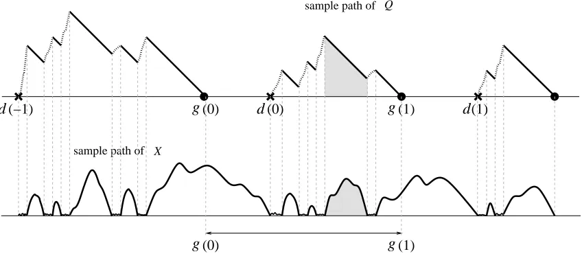
Q

sample path of

X

sample path of

g(1)

g(0)

g(0) g(1)

(−1) (0)

d d d(1)

Figure 1: Typical behaviour ofQand the background Markov process X when the underlying L´evy processY has unbounded variation paths. By convention, the origin of time is contained between g(0)and d(0). Note that excursions of X away from0 correspond to intervals over which Q decreases.

Lemma 2. Let(Ω,F_{, P)be a probability space endowed with aP-preserving flow(θt, t∈}R₎

[see Appendix A]. LetN1, N2be jointly stationary simple random point processes (Ni◦θt(B) =

Ni(B+t), t∈R, B∈B(R), i= 1,2) with points {ti(n), n∈Z}, i= 1,2, such that

· · ·< t1(−1)< t1(0)≤0< t1(1)< t1(2)<· · · ,

and

t1(n)< t2(n)< t1(n+ 1), for alln∈Z.

Let M be the random measure which is defined through its derivative with respect to the Lebesgue measure as

M(dt)/dt =X

n∈Z

1

Assume that N1 has finite intensity. Let PM be the Palm measure with respect to M. Then

EM[e−αt2(0)+βt1(0)] =

αEM[e−αt2(0)]−βEM[e−βt2(0)]

α−β , α, β >0. (25)

Proof. It is easy to see that M is also stationary, i.e.M◦θ_t(B) =M(B+t). Let P_Ni be the Palm measure with respect to Ni,i= 1,2 and let λbe the intensity ofN1 (which is–due to

the law of large numbers–the same as the intensity ofN2). It follows easily from Campbell’s

formula that M has finite intensity: λM = λEN1[t2(0)−t1(0)] < ∞. The Palm exchange formula2 _betweenP

M andPN1 yields

λMEM[Y] =λEN1 Z t1(1)

t1(0)

Y◦θ_t M(dt) =λE_N1 Z t2(0)

t1(0)

Y◦θ_tdt, (26)

2_{In [1] p. 21 the formula is given and proved for point processes but the generalization for arbitrary}

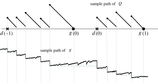
g(1) g(0)

Q

sample path of

(−1) (0)

d d

sample path of Y

Figure 2: Typical behaviour of Q and the background L´evy process Y, in case that Y is spectrally negative with bounded variation paths.

for any bounded random variable Y. Apply (26) with Y = e−αt2(0)+βt1(0)_{. Since t} 1(0) =

sup{t ≤ 0 : N1({t}) = 1}, t2(0) = inf{t > t1(0) : N2({t}) = 1}, and PN1(t1(0) = 0 <

t2(0)) = 1, we have t1(0)◦θt = −t, t2(0)◦θt = t2(0)−t, PN1-a.s. on {t1(0) < t < t2(0)}. Therefore, Y◦θ_t=e−αt1(0)_e(α−β)t_,P

N1-a.s. on{t1(0)< t < t2(0)}, and so

λMEM[e−αt2(0)+βt1(0)] =λ

EN1[e

−βt2(0)_]−E

N1[e −αt2(0)_]

α−β . (27)

Arguing in a similar manner, through the exchange formula between M and N2, we obtain

λMEM[e−βt2(0)+αt1(0)] =λ

EN2[e

αt1(0)_]−E

N2[e

βt1(0)_]

β−α . (28)

Settingβ = 0, and thenα = 0, in (27) we obtain:

λMEM[e−αt2(0)] =λ

1−EN1[e −αt2(0)_]

α ], (29)

λMEM[eβt1(0)] =λ

1−EN1[e−βt2(0)]

β . (30)

On the other hand, with α= 0 in (28), we have

λMEM[e−βt2(0)] =λ1−EN2[e βt1(0)_]

β . (31)

The exchange formula between N1 andN2 shows that the right hand sides of (30) and (31)

are equal. Substituting these and (29) into (27) we obtain the result.

5.1 Observed idle periods

We are interested in the distribution of the idle period (g(0), d(0)), given that Q0 = 0.

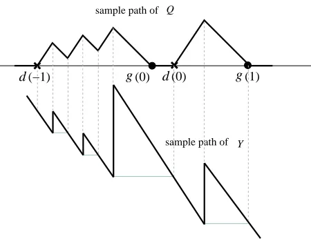
(0)

d

g(0) g(1)

sample path of Y

Q

sample path of

(−1)

d

Figure 3: Typical behaviour of Q and the background L´evy process Y, in case that Y is spectrally positive with bounded variation paths. Here, only the case where the jump part of

Y is compound Poisson is depicted. When Qt >0 and Xt= 0, we see that Qt increases at

rate |dY| −1, where dY <−1 is the drift of Y.

since this is an event with probability 1. If Q0 = 0 then Qt will remain 0 at least until X

hits 0, since Q cannot increase unless there is an accumulation of local time L, and this can happen only when X is 0. Recall that the first hitting time of 0 by X is denoted by

D= inf{t >0 :Xt= 0}. IfQ0 = 0, the first time thatQbecomes positive has been denoted

by d(0). Our claim is:

Lemma 3. Given that Q0 = 0 the ending time of the idle period is a.s. equal to D, i.e.,

P(d(0) =D|Q0= 0) = 1.

Proof. From the argument above we have that D ≤d(0) a.s. on {Q0 = 0}. Suppose that

there is Ω0⊂Ω with P(Ω0)>0 such thatQ0 = 0 andD < d(0) a.s. on Ω0. If Q0 = 0 and

D < d(0) then

Qt= sup D≤u≤t

{L(u, t]−(t−u)} ≡0, for all t∈(D, d(0)).

This implies that

L(u, t]≤t−u, for all D < u < t < d(0),

which means that, forω∈Ω0,L(ω,·) is absolutely continuous on some right neighbourhood

of D. IfY is spectrally negative or ifY is spectrally positive but not of bounded variation, thenL is a.s. singular on any right neighbourhood of D, and we obtain a contradiction. If

Y is spectrally positive with bounded variation paths then L is absolutely continuous and is given by (13). In this case, Q increases at rate |dY| −1 >0 whenever it is positive and

this shows immediately that here, too, D=d(0) a.s. on{Q0 = 0}.

Remark 1. The result in Lemma 3 can alternatively be expressed by saying that the process (Lt−t : t ≥ 0) is under P0 initially increasing. In [13] Proposition 6.3 this is proved in

Using Lemma 2, we shall reduce the problem to that of finding the distribution of

D = inf{t > 0 : Xt = 0} given that Q0 = 0. Let N1 (resp. N2) be the point process with

points{g(n} (resp.{d(n)}). ThenM(dt)/dt=

1

PM =P(· |Q0= 0).

Formula (25), together with Lemma 3, then gives

E[e−αd(0)+βg(0) |Q0 = 0] =

αE[e−αD|Q0 = 0]−βE[e−βD|Q0 = 0]

α−β . (32)

To compute the distribution ofD given Q0= 0 we need the following two lemmas.

Lemma 4. Let

G:= sup{t <0 : Xt= 0}.

Then it holds

{Q0= 0}={QG+G≤0}.

Proof. Since Xt>0 for allt∈(G, D), we have

L(s, t] = 0, G≤s≤t≤D.

Recall that

Qt=Rs,tLb(Qs) = sup s≤u≤t

b

L(u, t]∨ Qs+Lb(s, t]

So, ifG≤s≤t≤D, we have Lb(s, t] =L(s, t]−(t−s) =−(t−s), i.e.

Qt= (Qs−(t−s))+, G≤s≤t≤D.

If we assume thatQ0 = 0, we haveG≤g and so

0 =Qg = (QG−(g−G))+,

which implies that QG+G=g≤0.

Lemma 5. (i) Conditional on X0, the random variables QG, G, D are independent (under

P).

(ii) For all x≥0,t≥0,

P(QG> t) =Px(QG> t) =P0(Q0 > t) =e−θ ∗_t

.

where θ∗ = ψY(1) if Y is spectrally negative or is equal to the unique positive solution of

θ∗ _=ψ

Y(θ∗) ifY is spectrally positive.

(iii) QG is independent of(G, D) (under P).

Proof. (i) The independence follows from the strong Markov property at G (at which

XG = 0) and Markov property at 0. Indeed, first observe that G is a stopping time with

respect to the filtration {F_{t := σ(X−s,0 ≤ s ≤ t), t ≥ 0}. Second, QG = RG}e _Lb ₌

sup_s≤GLb(s, G] = sup_s≤G L(s, G]−(G−s)and soQG

1

to F′

t := σ(X−s, s > t) for all t. This proves independence between QG and G. Third, D

is measurable with respect to F′′

0 = σ(Xs, s ≥ 0). So, conditionally on X0, the random

follows from the strong Markov property at G. Let, as usual, F_{−G = {A ∈ σ(X−s, s ≥}

0) : A∩ {−G≤t} ∈F_{−t}. SinceQG=Q0}◦θ_G,

P(QG> t) =P(Q0◦θG> t) =EP(Q0◦θG> t|F−G) =EPXG(Q0 > t) =P0(Q0 > t) =e

−θ∗_t

where the latter follows from Theorem 3. (iii) This is immediate from (i) and (ii).

Proposition 5 (distribution of observed idle period). Fix α, β≥0, α6=β.

(i) When Y is spectrally negative we have

Ee−αd(0)+βg(0) |Q0= 0

= ΦY(0) 1−ΦY(0)

ψY(1)

α−β

α α−ψY(1)

ΦY(α)−1

ΦY(α) −

β β−ψY(1)

ΦY(β)−1

ΦY(β)

.

(ii) When Y is spectrally positive we have

Ee−αd(0)+βg(0) |Q0= 0= ψ

′

Y(0+)

1−ψ′

Y(0+)

θ∗ α−β

α−ΦY(α)

α−θ∗ −

β−ΦY(β)

β−θ∗

,

where θ∗ _{>0 is defined by ψ}

Y(θ∗) =θ∗.

Proof. From Lemma 5 we have that D, QG are conditionally independent given X0 and G.

Hence

E[e−θD

1

=E[e−θD|X0, G] (1−eθ ∗_G

)

=E[e−θD−e−θD+θ∗G|X0, G],

where the second line was obtained from the facts (all consequences of Lemma 5) that (i)

D, Gare conditionally independent given X0, (ii)QG, Gare also conditionally independent

given X0, and (iii) QG is independent of X0 and exponentially distributed with parameter

θ∗= (

ψY(1), ifY is spectrally negative

ψY(θ∗), ifY is spectrally positive

(33)

Taking expectations we get

E[e−θD

1

and, using Lemma 4,

E[e−θD |Q0= 0] =

E[e−θD]−E[e−θD+θ∗G]

P(Q0= 0)

.

We now use a version of Lemma 2, formulated for excursions of general stationary processes; Pitman [14, Corollary p. 298; references therein]. The random measuresN1, N2 correspond

to the beginnings and ends of excursions of the stationary process (Xt, t ∈ R), and, since

the Lebesgue measure, while PM = P. Applying Pitman’s result–an analogue of formula

(25)–gives

E[e−αD+βG] = αE[e

−αD_]−βE[e−βD_]

α−β . (34)

The joint Laplace transform of D, G is thus expressible in terms of the Laplace transform of D. Combining the last two displays we obtain:

E[e−θD|Q0 = 0] =

1

P(Q0= 0)

θ∗ θ−θ∗

n

E[e−θ∗D]−E[e−θD]o.

Using this in (32) results in

E[e−αd(0)+βg(0) |Q0= 0] = 1

P(Q0 = 0)

θ∗ α−β

×

α

α−θ∗ E[e −θ∗_D

]−E[e−αD]− β

β−θ∗ E[e −θ∗_D

]−E[e−βD]

(35)

So far, the arguments are general and hold for both spectrally negative and positive L´evy processes Y, as long as θ∗ is taken as in (33). Substituting next the expression for the Laplace transform of D from (8), (16) for the spectrally negative, respectively positive, case, we obtain the result.

5.2 Observed busy periods

In this section we follow ideas in [16]. We are interested in the distribution of the observed busy period, as defined in (24). On the conditioning event {Q0 > 0}, we have, by our

enumeration convention,

g(0)< d(0)<0< g(1), P−a.s.

Using Lemma 2 with N1 (resp. N2) the point process with points {d(n)}(resp. {g(n}), we

have

E[e−αg(1)+βd(0) |Q0 >0] = αE[e

−αg(1) _|Q

0 >0]−βE[e−βg(1) |Q0>0]

α−β , α, β >0. (36)

Recall the evolution equation forQ:

Qt=Qs+L(s, t]−(t−s)− inf

s≤u≤t{Qs+L(s, u]−(u−s)}. (37)

Lets= 0 and assumeQ0 >0. SinceX0>0,P-a.s., we haveL(0, t] = 0 for all 0< t < D=

inf{r >0 :Xr = 0}, and so,

Qt=Q0−t− inf

0≤u≤t{Q0−u}=Q0−t, a.s. on {Q0 >0, t < D},

which implies that

g(1) = (

Q0, a.s. on{0< Q0 < D},

g(1)◦θD, a.s. on{Q0 > D}.

Now, if Q0> D, we have QD−=Q0−D, so from (37),Q evolves as

QD+t=Q0−D+L[D, D+t]−t, t≥0,

ans as long as QD+t>0. This implies that, a.s. on{Q0> D},

g(1)◦θD−D= inf{t >0 : Q0−D+L[D, D+t]−t= 0}.

Therefore (38) becomes

g(1) = (

Q0, a.s. on {0< Q0< D},

D+ inf{t >0 : Q0−D+L[D, D+t]−t= 0}, a.s. on {Q0 > D}.

(39)

Consider now the inverse local time process, with the origin of time placed atD, i.e.

L−_D1_;x := inf{t >0 : L[D, D+t]> x}, x≥0.

By the strong Markov property forXat the stopping timeDwe have that theP-distribution of (L−_D1_;x, x≥0) is the same as theP0-distribution of (L−x1, x≥0), which has been identified

in Propositions 2 and 4: Thus, (L−_D1_;x, x≥0) is a (proper) subordinator. Consider next the spectrally negative L´evy process

e

Λx:=x−L−D1;x, x≥0.

Notice that P(Λe0 = 1). The Laplace exponent of Λ is the functione ψΛ of (22). Define the

hitting time of level −abyΛe

σ(Λ;e a) := inf{x >0 : Λex <−a}, a >0,

Formula (61) gives us the Laplace transform of σ(Λ;e a) in terms of the scale functions of Λ,e defined in (56) and (57). Combining them, we obtain

Z ∞

0

e−θa E[e−qσ(Λ;ea)]da= 1

ψΛ(θ)−q

ψΛ(θ)

θ −

q

ΦΛ(θ)

=:H(q)(θ). (40)

As can be easily seen from Lemma 1, for anya >0,

inf{t >0 : t−L[D, D+t]≥a}= inf{x >0 : Λex <−a}+a=σ(Λ;e a) +a.

Using this in (39), we obtain

g(1) = (

Q0, a.s. on {0< Q0 < D},

Q0+σ(Λ;e Q0−D), a.s. on {Q0 > D}.

It is useful to keep in mind thatΛ is independent ofe Q0−D, by the strong Markov property

of X at D. We are now ready to compute the Laplace transform appearing on the right hand side of (36):

E[e−αg(1);Q0>0] =E[e−αg(1); 0< Q0 < D] +E[e−αg(1);Q0 > D]

=E[e−αQ0_{; 0< Q}

0< D] +E[e−α(Q0+σ(Λ;eQ0−D);Q0 > D]

=E[e−αQ0_;Q

Recall that P(Q0 > x) =µe−θ ∗_x

, and so

E[e−αQ0_;Q

0 >0] =µ θ

∗

α+θ∗. (42)

To compute the second and the third terms we need some elementary properties of expo-nentially distributed random variables which we state without proof.

Lemma 6. Let T be an exponentially distributed r.v. with parameter λand(X, Y), X≥0,

Y ≥0, be a two-dimensional r.v. independent ofT. ThenX andT−X−Y are independent given T > X+Y. Moreover,

E[e−α(T−X−Y)|T > X+Y] = λ

α+λ,

E[e−αX;T > X+Y] =E[e−(α+λ)X−λY].

Use (37) once more with s=G= sup{t <0 : Xt = 0}, andt= 0, taking into account

the fact that L is not supported on (G,0), to obtain

Q0 =QG+G, a.s. on{Q0 >0}.

Since QG is exponentially distributed with parameter θ∗ and independent of (G, D) (from

Lemma 5), we have, applying Lemma 6, the following result:

Lemma 7. Given Q0> D, the r.v.’s Q0−Dand D are independent. Moreover,

E[e−α(Q0−D)_|Q

0 > D] =

θ∗ α+θ∗,

E[e−αD;Q0 > D] =E[e−(α+θ

∗_)D+θ∗_G

].

Using Lemma 7, we write the last term of (41) as follows:

E[e−αQ0 _(1−e−ασ(Λ;eQ0−D)_);Q 0 > D]

=P(Q0> D)E[e−αD e−α(Q0−D) (1−e−ασ(Λ;eQ0−D))|Q0> D]

=P(Q0> D)E[e−αD |Q0> D]E[e−α(Q0−D) (1−e−ασ(Λ;eQ0−D))|Q0> D]

=E[e−(α+θ∗)D+θ∗G]E[e−αV (1−e−ασ(eΛ;V))], (43)

where, in the last term, we introduced a random variableV, exponentially distributed with parameterθ∗, independent of everything else (due to the fact thatQ0−D, conditionally on

being positive, is exponential with parameter θ∗_{, independent ofΛ). The first term of (43)e} can be computed as in (34). We have, for all α, β ≥0, α6=β,

E[e−αD+βG] = ΦY(0)

α−β

_α

ΦY(α)

− β

ΦY(β)

,

and for the spectrally positive case, for allα, β ≥0, α6=β,

E[e−αD+βG] =ψ′_Y(0+)ΦY(α)−ΦY(β)

Note that taking account of the definition (22) of ψΛ for both the spectrally negative and

positive cases, and the fact that ψΛ(θ∗) = 0, one sees that generically for both cases, for all

α≥0,

E[e−(α+θ∗)D+θ∗G] = µ

α(α−ψΛ(α+θ

∗_{)). (44)}

For the second term of (43) we have, using (40),

E[e−αV(1−e−ασ(Λ;eV))] = θ ∗

α+θ∗ −θ ∗Z ∞

0

e−θ∗ve−αvE[e−ασ(Λ;ev)]dv

= θ ∗

α+θ∗ −θ

∗_H(α)_(α+θ∗₎

= θ ∗

α+θ∗ −

θ∗

ψΛ(α+θ∗)−α

_ψ

Λ(α+θ∗)

α+θ∗ −

α

ΦΛ(α)

= θ ∗

α+θ∗

α+θ∗_−Φ

Λ(α)

ΦΛ(α)

α ψΛ(α+θ∗)−α

(45)

Multiplying (44) and (45) we obtain the following expression for (43):

E[e−αQ0_(1−e−ασ(Λ;eQ0−D)_);Q

0 > D] =

µθ∗

α+θ∗ −

µθ∗ ΦΛ(α)

This, together with (42) and (41), yields:

E[e−αg(1) |Q0>0] = θ

∗ ΦΛ(α)

.

Using (36), we finally come to rest at the following main result.

Proposition 6 (distribution of observed busy period). For α, β >0, α6=β,

E[e−αg(1)+βd(0)|Q0>0] =

θ∗ α−β

_α

ΦΛ(α) −

β

ΦΛ(β)

where ΦΛ is the right inverse of ψΛ which is given in (22) and (cf. Theorem 3)

(i) θ∗ >0 is defined by ψY(1) in the case thatY is spectrally negative,

(ii) θ∗>0 is defined by ψY(θ∗) =θ∗ in the case that Y is spectrally positive.

5.3 Typical idle and busy periods

We now consider the problem of identifying the distribution of a typical idle and a typical busy period of Q. We place the origin of time at the beginning of such a period, by considering the appropriate Palm probability. Let Ng (resp.Nd) be the point process with

points{g(n)} (resp.{d(n)}), the beginnings of idle (resp. of busy) periods, and letPg (resp.

Pd) be the Palm probability with respect toNg (resp. Pd).

(0)

Using (29) we have

1−µ λ αE[e

−αd(0)_|Q

0= 0] = 1−Eg[e−αd(0)],

where µ=P(Q0 >0) and λis the common rate of Ng and Nd. The right side is precisely

what we need. Everything in the left side is known (see Prop. 5) except the rateλ. Consider first the case whenY is spectrally negative. Using Prop. 5(i) withβ = 0 we get

1−µ λ

ΦY(0)

1−ΦY(0)

ψY(1)

α α−ψY(1)

ΦY(α)−1

ΦY(α)

= 1−Eg[e−αd(0)].

Taking limits as α → ∞–and since ΦY(α)→ ∞–we find the value of λand so the Laplace

transformEg[e−αd(0)] of the typical idle period. The result is in Proposition 7(i) below.

We repeat the procedure for the spectrally positive case and, using Proposition 5(ii), we obtain:

1−µ λ

ψ_Y′ (0) 1−ψ′

Y(0)

θ∗α−ΦY(α)

α−θ∗ = 1−Eg[e

−αd(0)_].

Note that limθ→∞ψY(θ)/θ=∞if Y is of unbounded variation, and so limα→∞ΦY(α)/α=

0. Thus, we can findλand Eg[e−αd(0)]–see Proposition (7)(ii) below.

But ifY is spectrally positive (with non-monotone paths) and of bounded variation then

L is absolutely continuous and has a drift dY–see (13). We can easily see, e.g. from (12),

that

ψY(θ) = logE[e−θ(Y1−Y0)] =|dY|θ−

Z ∞

0

(1−e−θy)Π(dy),

and, sinceR₀∞(y∧1)Π(dy)<∞, we obtain limθ→∞ψY(θ)/θ=|dY|. So limα→∞ΦY(α)/α=

1/|dY|. Again, we can findλand Eg[e−αd(0)]–see Proposition (7)(iii) below.

Proposition 7 (distribution of typical idle period). Fix α >0. Let Pg be Palm probability

with respect to the beginnings of idle periods of Q.

(i) When Y is spectrally negative we have

λ= ΦY(0)ψY(1), Eg[e−αd(0)] = 1− α

ΦY(α)

ΦY(α)−1

α−ψY(1)

.

(ii) When Y is spectrally positive andR₀1yΠ(dy) =∞, we have

λ=ψ_Y′ (0)θ∗, Eg[e−αd(0)] = 1−θ∗

α−ΦY(α)

α−θ∗ ,

where θ∗ >0 satisfies θ∗=ψY(θ∗).

(iii) When Y is spectrally positive andR₀1yΠ(dy)<∞, we have

λ=ψ′_Y(0)θ∗

1− 1

|dY|

, Eg[e−αd(0)] = 1−

θ∗ 1− 1

|dY|

α−ΦY(α)

α−θ∗ ,

where θ∗ >0 satisfies θ∗=ψY(θ∗), and dY is the drift defined in (12)-(13).

Remark 2. By Assumption [A2]–see Section 3–we havedY <−1 and so the constant above

In the same vein, we obtain the Laplace transform Ed[e−αg(1)] of a typical busy period.

Notice that, under Pd, we have d(0) = 0, and so the first busy period to the right of the

origin of time is the interval (d(0), g(1)). We have,

µ λαE[e

−αg(1)_|Q

0 >0] = 1−Ed[e−αg(1)].

Using Proposition 6 withβ = 0, we have

µθ∗ λ

α

ΦΛ(α)

= 1−Ed[e−αg(1)].

From the expression (22) forψΛ(θ) we find limθ→∞ψΛ(θ)/θ= 1. So, limα→∞α/ΦΛ(α) = 1.

Therefore:

Proposition 8 (distribution of typical busy period). Fixα >0. LetPd be Palm probability

with respect to the beginnings of busy periods of Q. LetψΛ be defined as in (22), and letΦΛ

be its right inverse function. Then

λ=µθ∗, Ed[e−αg(1)] = 1−

α

ΦΛ(α)

,

where µ= ΦY(0), θ∗=ψY(1), if Y is spectrally negative; and µ=ψ′Y(0), θ∗>0 is defined

through θ∗_=ψ

Y(θ∗), if Y is spectrally positive.

Corollary 1. The mean duration of a typical idle period is(1−µ)/λ, while the mean dura-tion of a typical busy period isµ/λ, whereµ is given by (17) andλis given in Propositions 7, 8.

Remark 3. By the relation between P and the Palm probability Pd it follows that the

typical idle (respectively busy) periods are stochastically smaller than the observed idle (respectively busy) periods, see [1]. In particular, the means of the former are shorter than the means of the latter. (This is usually referred to as the “inspection paradox”.) This gives us several inequalities between different quantities associated with the L´evy process Y. To give an example, we compare the mean durations of idle periods in the spectrally negative case. From Proposition 5 we have

Ee−αd(0) |Q0= 0=

ΦY(0)ψY(1)

1−ΦY(0)

ΦY(α)−1

ΦY(α)(α−ψY(1))

=: ΦY(0)ψY(1) 1−ΦY(0)

F(α).

It follows that

Ed(0)|Q0 = 0=−

ΦY(0)ψY(1)

1−ΦY(0)

F′(0).

Since d(0) and−g(0) are identical in law, the mean duration of the observed idle period is

Ed(0)−g(0)|Q0 = 0=−2ΦY(0)ψY(1)

1−ΦY(0)

F′(0).

Notice that, using the functionF,we may write from Proposition 7

and

Eg[d(0)] =F(0).

Now, by the “inspection paradox”,

Eg[d(0)]≤Ed(0)−g(0)|Q0 = 0,

which, after some manipulations, is equivalent with

(1−ΦY(0))2 ≤2 ΦY(0)2−ΦY(0) + Φ′Y(0)ψY(1).

Example 5 (continuation of Example 1): Consider Yt = σBt−µt, and assume 0 <

µ <1. Here the rate of beginnings of idle (or busy) periods is

λ=ψ_Y′ (0)θ∗ = 2µ(1−µ)

σ2 .

The mean duration of a typical idle period of Qis

σ2

2µ,

while the mean duration of a typical busy period ofQ is

σ2

2(1−µ).

To find, e.g., the distribution of a typical busy period, we use Proposition 8. We have, see (22),

ψΛ(q) =q−ΦY(q),

where ΦY is the inverse function ofψY, i.e.

ΦY(q) =

p

µ2_{+ 2σ}2_q2_−µ

σ2 ,

and ΦΛ is the inverse function ofψΛ, i.e.

ΦΛ(α) =

(1−µ) + 2σ2α+p(1−µ)2_{+ 4σ}2_α

2σ2 ,

and so the Laplace transform of the typical busy period is

Ed[e−αg(1)] =

(1−µ) +p(1−µ)2_{+ 4σ}2_α

(1−µ) + 2σ2_α+p_(1−µ)2_{+ 4σ}2_α.

A

On Skorokhod reflection, fluid queues, and stationarity

it is nevertheless interesting to isolate those properties that are not based on specific dis-tributional assumptions (such as Markovian property or independent increments) but are consequences the more general stationary framework.

Let (Ω,F_{, P) be a probability space together with aP-preserving flow (θt, t∈}R_{). That}

is, for each t ∈ R_{, θt : Ω → Ω is measurable with measurable inverse, θ0 is the identity}

function,θt◦θs =θs+t, for alls, t∈R, andP(θtA) =P(A) for all t∈R,A∈F. Consider a

processW = (Wt, t∈R) with stationary increments, i.e. (Wt−Ws)◦θu=Wt+u−Ws+u for

all s, t, u∈R_{. We let E denote expectation with respect toP.}

Following [8], we define the“Skorokhod Dynamical System” (abbreviated SDS henceforth) driven by W as a 2-parameter stochastic flow:

Rs,tW(x) := [x+Wt−Ws]− inf

s≤u≤t[(x+Ws−Wu)∧0] (46)

:= sup

s≤u≤t

(Wt−Wu)∨(x+Wt−Ws) x≥0, s≤t. (47)

Thus, for each s < t, we have a random elementRs,tW taking values in the space ofC(R₊₎

of continuous functions from R_{+ into itself. The family (Rs,tW, − ∞ < s < t <∞) is a}

stochastic flowbecause the following composition rule (semigroup property) holds for each

ω∈Ω:

Rs,tW=Ru,tW◦Rs,u_W, s≤u≤t,

Rt,tW(x) =x, t∈R_{, x≥0,}

It is a stationary stochastic flow because, for each x∈R_{+, we have:}

Rs,tW(x)◦θu=Rs+u,t+uW(x), − ∞< s≤t <∞, u∈R.

We say that the processZ=Zt, t∈R constitutes a stationary solution of the SDS driven

by W if Zis W-measurable and if

Zt=Rs,tW(Zs), s≤t,

Zt◦θu =Zt+u, t, u∈R.

Existence and uniqueness is guaranteed under some assumptions:

Lemma 8. Assume that sup_−∞<s≤0Ws <∞, and limt→∞Wt <∞, P-a.s. Then there is

a unique stationary solution to the Skorokhod dynamical system driven by W. This is given by

Zt= sup

−∞<u≤t

(Wt−Wu) =:Rte W. (48)

Quite often, in addition to stationarity of the flow, we also also assume ergodicity, namely that each A ∈ F _{that is invariant under θt for all t, has P(A) equal to 0 or 1. Owing to}

Birkhhoff’s individual ergodic theorem Lemma 8 immediately yields:

Corollary 2. Under the ergodicity assumption, and if EW1 < 0, then there is a unique

For the purposes of this paper, assume that W is of the form

Wt−Ws=A(s, t]−β(t−s), s≤t, (49)

whereA is a locally finite stationary random measure, and

0< β < α:=EA(0,1). (50)

LetPA be the Palm probability, see [1], [6], with respect toA:

PA(C) = 1

αE

Z

(0,1]

1

.

The following is a consequence of Theorem 3 of [8]:

Lemma 9 (distributional Little’s law). Let Z be the unique stationary solution to the SDS driven byW of the form (49). Assume that (50) holds. Then, for any functionψ: [0,∞)→ R_{, which is continuous on (0,∞), we have (Theorem 3 of [8])}

Eψ(Z0) =

1− α

β

ψ(0) + α

βEAψ(Z0).

In particular,

P(Z0 > x) = α

βPA(Z0> x), x >0, P(Z0>0) = α

β. (51)

It should be noted that the decomposition (49) of W is not unique; nevertheless, (51) holds, regardless of which decomposition of W we choose.

B

Exit times for spectrally negative L´

evy processes

In this section we consider a spectrally negative L´evy process and some facts regarding the first time the process exits an unbounded interval. Let Y = (Yt, t ∈ R) be a spectrally

negative L´evy process and L´evy measure Π. In other words, letB be a standard Brownian motion, η an independent Poisson random measure on R_×R_{− such that}

Eη(dt, dy) =dtΠ(dy), Π{0}= 0,

Z

R−

(y2∧1)Π(dy) <∞, (52)

let a∈R_{,σ ≥0, and define, for −∞< s≤t <∞,}

Y(s, t] =a(t−s) +σ(Bt−Bs)

+ Z

(s,t] Z

(−∞,−1]

y η(du, dy) + Z

(s,t] Z

(−1,0)

y [η(du, dy)−duΠ(dy)]. (53)

Notice that we have thus defined only the increments of Y; the exact value of Y0 is

unim-portant; we may, arbitrarily, set