Scalable Planning and Learning for Multiagent POMDPs: Extended Version

Scalable Planning and Learning for Multiagent POMDPs:

Extended Version

Christopher Amato

CSAIL, MIT

Cambridge, MA 02139

[email protected]

Frans A. Oliehoek

Informatics Institute, University of Amsterdam

Dept. of CS, University of Liverpool

[email protected]

Abstract

Online, sample-based planning algorithms for POMDPs have shown great promise in scaling to problems with large state spaces, but they become intractable for large action and observation spaces. This is partic-ularly problematic in multiagent POMDPs where the action and observation space grows exponentially with the number of agents. To combat this intractability, we propose a novel scalable approach based on sample-based planning and factored value functions that exploits structure present in many multiagent settings. This approach applies not only in the planning case, but also in the Bayesian reinforcement learning setting. Ex-perimental results show that we are able to provide high quality solutions to large multiagent planning and learning problems.

1

Introduction

Online planning methods for POMDPs have demonstrated impressive performance (Ross et al., 2008) on large problems by interleaving planning with action selection. The leading such method, partially observable Monte Carlo planning (POMCP) (Silver and Veness, 2010), achieves performance gains by extending sample-based methods based on Monte Carlo tree search (MCTS) to solve POMDPs.

While online, sample-based methods show promise in solving POMDPs with large state spaces, they be-come intractable as the number of actions or observations grow. This is particularly problematic in the case of multiagent systems. Specifically, we consider multiagent partially observable Markov decision processes (MPOMDPs), which assume all agents share the same partially observable view of the world and can coordi-nate their actions. Because the MPOMDP model is centralized, POMDP methods apply, but the fact that the number ofjointactions and observations scales exponentially in the number of agents renders current POMDP methods intractable.

To combat this intractability, we provide a novel sample-based online planning algorithm that exploits mul-tiagent structure. Our method, calledfactored-value partially observable Monte Carlo planning (FV-POMCP), is based on POMCP and is the first MCTS method that exploitslocality of interaction: in many MASs, agents interact directly with a subset of other agents. This structure enables a decomposition of the value function into a set of overlapping factors, which can be used to produce high quality solutions (Guestrin, Koller, and Parr, 2001; Nair et al., 2005; Kok and Vlassis, 2006). But unlike these previous approaches, we will not assume a factored model, but only that the value function can be approximately factored. We present two variants of FV-POMCP that use different amounts of factorization of the value function to scale to large action and observation spaces.

Not only is our FV-POMCP approach applicable to large MPOMDPs, but it is potentially even more im-portant for Bayesian learning where the agents have uncertainty about the underlying model as modeled by Bayes-Adaptive POMDPs (BA-POMDPs) (Ross et al., 2011). These models translate the learning problem to a planning problem, but since the resulting planning problems have an infinite number of states, scalable sample-based planning approaches are critical to their solution.

1

We show experimentally that our approach allows both planning and learning to be significantly more efficient in multiagent POMDPs. This evaluation shows that our approach significantly outperforms regular (non-factored) POMCP, indicating that FV-POMCP is able to effectively exploit locality of interaction in both settings.

2

Background

We first discuss multiagent POMDPs and previous work on Monte Carlo tree search and Bayesian reinforcement learning (BRL) for POMDPs.

2.1

Multiagent POMDPs

An MPOMDP (Messias, Spaan, and Lima, 2011) is a multiagent planning model that unfolds over a number of steps. At every stage, agents take individual actions and receive individual observations. However, in an MPOMDP, all individual observations are shared via communication, allowing the team of agents to act in a ‘centralized manner’. We will restrict ourselves to the setting where such communication is free of noise, costs and delays.

An MPOMDP is a tuplehI, S,{Ai}, T, R,{Zi}, O, hiwith: I, a set of agents; S, a set of states with

designated initial state distributionb0;A= ×iAi, the set of joint actions, using action sets for each agent,i;

T, a set of state transition probabilities: Ts~as0 _{= Pr(s}0_{|s, ~a), the probability of transitioning from statestos}0

when actions~aare taken by the agents;R, a reward function:R(s, ~a), the immediate reward for being in states and taking actions~a;Z =×iZi, the set of joint observations, using observation sets for each agent,i;O, a set

of observation probabilities:O~as0~z_{= Pr(~z|~a,s}0_{), the probability of seeing observations~ogiven actions~awere}

taken and resulting states0;h, the horizon.

An MPOMDP can be reduced to a POMDP with a single centralized controller that takes joint actions and receives joint observations (Pynadath and Tambe, 2002). Therefore, MPOMDPs can be solved with POMDP solution methods, some of which will be described in the remainder of this section. However, such approaches do not exploit the particular structure inherent to many MASs. In Sec. 4, we present a first online planning method that overcomes this deficiency.

2.2

Monte Carlo Tree Search for (M)POMDPs

Most research for (mutliagent) POMDPs has focused onplanning: given a full specification of the model, determine an optimal policy,π, mapping past observation histories (which can be summarized by distributions b(s)over states called beliefs) to actions. An optimal policy can be extracted from an optimal Q-value function, Q(b,a) = P

sR(s,a) +

P

zP(z|b,a) maxa0Q(b

0_,a0_{), by acting greedily. ComputingQ(b,a), however, is}

complicated by the fact that the space of beliefs is continuous.

2.3

Bayesian RL for (M)POMDPs

Reinforcement learning (RL)considers the more realistic case where the model is not (perfectly) known in advance. Unfortunately, effective RL in POMDPs is very difficult. Ross et al. (2011) introduced a framework, called the Bayes-Adaptive POMDP (BA-POMDP), that reduces the learning problem to a planning problem, thus enabling advances in planning methods to be used in the learning problem.

In particular, the BA-POMDP utilizes Dirichlet distributions to model uncertainty over transitions and ob-servations. Intuitively, if the agent could observe states and observations, it could maintain vectorsφandψ of counts for transitions and observations respectively. Letφa_ss0 be the transition count of the number times

states0resulted from taking actionain statesandψ_sa0_zbe the observation count representing the number of

times observationzwas seen after taking actionaand transitioning to states0. These counts induce a proba-bility distribution over the possible transition and observation models. Even though the agent cannot observe the states and has uncertainty about the actual count vectors, this uncertainty can be represented using the POMDP formalism— by including the count vectors as part of the hidden state of a special POMDP, called a BA-POMDP.

The BA-POMDP can be extended to the multiagent setting (Amato and Oliehoek, 2013), yielding the Bayes-Adaptive multiagent POMDP (BA-MPOMDP) framework. BA-MPOMDPs are POMDPs, but with an infinite state space since there can be infinitely many count vectors. While a quality-bounded reduction to a finite state space is possible (Ross et al., 2011), the problem is still intractable; sample-based planning is needed to provide solutions. Unfortunately, current methods, such as POMCP, do not scale well to multiple agents.

3

Exploiting Graphical Structure

POMCP is not directly suitable for multiagent problems (in either the planning or learning setting) due to the fact that the number of joint actions and observations are exponential in the number of agents. We first elaborate on these problems, and then sketch an approach to mitigate them by exploiting locality between agents.

3.1

POMCP for MPOMDPs: Bottlenecks

The large number of joint observations is problematic since it leads to a lookahead tree with very high branching factor. Even though this is theoretically not a problem in MDPs (Kearns, Mansour, and Ng, 2002), in partially observable settings that use particle filters it leads to severe problems. In particular, in order to have a good particle representation at the next time step, the actual joint observation received must be sampled often enough during planning for the previous stage. If the actual joint observation had not been sampled frequently enough (or not at all), the particle filter will be a bad approximation (or collapse). This results in sampling starting from the initial belief again, or alternatively, to fall back to acting using a separate (history independent) policy such as a random one.

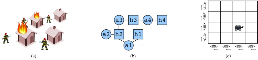
The issue of large numbers of joint actions is also problematic: the standard POMCP algorithm will, at each node, maintain separate statistics, and thus separate upper confidence bounds, for each of the exponentially many joint actions. Each of the exponentially many joint actions will have to be selected at least a few times to reduce their confidence bounds (i.e., exploration bonus). This is a principled problem: in cases where each combination of individual actions may lead to completely different effects, it may be necessary to try all of them at least a few times. In many cases, however, the effect of a joint action is factorizable as the effects of the action of individual agents or small groups of agents. For instance, consider a team of agents that is fighting fires at a number of burning houses, as illustrated in Fig. 1(a). The rewards depend only on the amount of water deposited on each house rather than the exact joint action taken (Oliehoek et al., 2008). While this problem lends itself to a natural factorization, other problems may also be factorized to permit approximation.

3.2

Coordination Graphs

In certain multiagent settings,coordination (hyper) graphs (CGs)(Guestrin, Koller, and Parr, 2001; Nair et al., 2005) have been used to compactly represents interactions between subsets of agents. In this paper we extend

(a) (b) (c)

Figure 1: (a) Illustration of ‘fire fighting’ (b) Coordination graph with 4 houses and 3 agents (c) Illustration of a sensor network problem on a grid that is used in the experiments.

this approach to MPOMDPs. We first introduce the framework of CGs in the single shot setting.

A CG specifies a set of payoff componentsE ={Qe}, and each componenteis associated with a subset

of agents. These subsets (which we also denote usinge) can be interpreted as (hyper)-edges in a graph where the nodes are agents. The goal in a CG is to select a joint action that maximizes the sum of the local payoff componentsQ(~a) = P

eQe(~ae).

1 _{A CG for the fire fighting problem is shown in Fig. 1(b). We follow the}

cited literature in assuming that a suitable factorization is easily identifiable by the designer, but it may also be learnable. Even if a payoff functionQ(~a)does not factor exactly, it can be approximated by a CG. For the moment assuming astateless problem(we will consider the case where histories are included in the next section), an action-value function can be approximated by

Q(~a)≈X e

Qe(~ae), (1)

We refer to this as the linear approximation ofQ, since one can show that this corresponds to an instance of linear regression (See Sec. 5).

Using a factored representation, the maximizationmax~aPeQe(~ae)can be performed efficiently via

vari-able elimination (VE) (Guestrin, Koller, and Parr, 2001), or max-sum (Kok and Vlassis, 2006). These algo-rithms are not exponential in the number of agents, and therefore enable significant speed-ups for larger number of agents. The VE algorithm (which we use in the experiments) is exponential in theinduced widthwof the coordination graph.

3.3

Mixture of Experts Optimization

VE can be applied if the CG is given in advance. When we try to exploit these techniques in the context of POMCP, however, this is not the case. As such, the task we consider here is to find the maximum of anestimated factored functionQˆ(~a) = P

eQˆe(~ae). Note that we do not necessarily require the best approximation to the

entireQ, as in (1). Instead, we seek an estimationQˆfor which the maximizing joint action~aM _{is close to the}

maximum of the actual (but unknown) Q-value:Q(~aM_)≈Q(~a∗_).

For this purpose, we introduce a technique calledmixture of experts optimization. In contrast to methods based on linear approximation (1), we do not try to learn a best-fit factored Q function, but directly try to estimate the maximizing joint action. The main idea is that for each local action~aewe introduce an expert that predicts

thetotalvalueQˆ(~ae) =E[Q(~a)|~ae]. For a joint action, these responses—one of each payoff componente—

are put in a mixture with weightsαeand used to predict the maximization joint action:arg max~aPeαeQˆ(~ae).

This equation is the sum of restricted-scope functions, which is identical to the case of linear approximation (1), so VE can be used to perform this maximization effectively. In the remainder of this paper, we will integrate the weights and simply writeQˆe(~ae) =αeQˆ(~ae).

1_{Since we focus on the one-shot setting here, the Q-values in the remainder of this section should be interpreted as those for one specific}

~a1

~ o1

~a2

~ o1

~a2

~

o1 _~o2

Figure 2: Factored Statistics: joint histories are maintained (for specific joint actions and observations specified by~aj_and~ok_{), but action statistics are factored at each node.}

The experts themselves are implemented as maximum-likelihood estimators of the total value. That is, each expert (associated with a particular~ae) keeps track of the mean payoff received when~aewas performed, which

can be done very efficiently. An additional benefit of this approach is that it allows for efficient estimation of upper confidence bounds by also keeping track of how often this local action was performed, which in turns facilitates easy integration in POMCP, as we describe next.

4

Factored-Value POMCP

This section presents our main algorithmic contribution: Factored-Value POMCP, which is an online planning method for POMDPs that can exploit approximate structure in the value function by applying mixture of ex-perts optimization in the POMCP lookahead search tree. We introduce two variants of FV-POMCP. The first technique,factored statistics, only addresses the complexity introduced by joint actions. The second technique, factored trees, additionally addresses the problem of many joint observations. FV-POMCP is the first MCTS method to exploit structure in MASs, achieving better sample complexity by using factorization to generalize the value function over joint actions and histories. While this method was developed to scale POMCP to larger MPOMDPs in terms of number of agents, the techniques may be beneficial in other multiagent models and other factored POMDPs.

4.1

Factored Statistics

We first introduceFactored Statisticswhich directly applies mixture of experts optimization to each node in the POMCP search tree. As shown in Fig. 2, the tree of joint histories remains the same, but the statistics retained at for each history is now different. That is, rather than maintaining one set of statistics in each node (i.e, joint history~h) for the expected value of each joint actionQ(~h,~a), we maintain a set of statistic for each component ethat estimates the valuesQe(~h,~ae)and corresponding upper confidence bounds.

Joint actions are selected according to the maximum (factored) upper confidence bound:

max

~ a

X

e

Ue(~h,~ae),

WhereUe(~h,~ae),Qe(~h,~ae) +cplog(N~_h+ 1)/n~aeusing the Q-value and the exploration bonus added for

that factor. For implementation, at each node for a joint history~h, we store the count for the full historyN~_has

well as the Q-values,Qe, and the counts for actions,n~ae, separately for each componente.

Since this method retains fewer statistics and performs joint action selection more efficiently via VE, we expect that it will be more efficient than plain application of POMCP to the BA-MPOMDP. However, the complexity due to joint observations is not directly addressed: because joint histories are used, reuse of nodes

. . .

e

. . .

~a1 1

~ o1

1

~a2 1

~ o1

1

~a2 1

~ o1

1 ~o21

~a1 |E|

~ o1

|E|

~a2 |E|

~ o1

|E|

~a2 |E|

~ o1

|E| ~ o2

|E|

Figure 3: Factored Trees: local histories for are maintained for each factor (resulting in factored history and action statistics). Actions and observations for componentiare represented as~aj_i and~ok

i)

and creation of new nodes for all possible histories (including the one that will be realized) may be limited if the number of joint observations is large.

4.2

Factored Trees

The second technique, calledFactored Trees, additionally tries to overcome the large number of joint observa-tions. It further decomposes the localQe’s by splitting joint histories into local histories and distributing them

over the factors. That is, in this case, we introduce an expert for each local~he, ~aepair. During simulations, the

agents know~hand action selection is conducted by maximizing over the sum of the upper confidence bounds:

max

~ a

X

e

Ue(~he, ~ae),

whereUe(~he, ~ae) =Qe(~he, ~ae) +c q

log(N~_h

e+ 1)/n~ae. We assume that the set of agents with relevant actions

and histories for componentQe are the same, but this can be generalized. This approach further reduces the

number of statistics maintained and increases the reuse of nodes in MCTS and the chance that nodes in the trees will exist for observations that are seen during execution. As such, it can increase performance by increasing generalization as well as producing more robust particle filters.

This type of factorization has a major effect on the implementation: rather than constructing a single tree, we now construct a number of trees in parallel, one for each factoreas shown in Fig. 3. A node of the tree for componentenow stores the required statistics:N~_he, the count for the local history,n~ae, the counts for actions

taken in the local tree andQefor the tree. Finally, we point out that this decentralization of statistics has the

potential to reduce communication since the components statistics in a decentralized fashion could be updated without knowledge of all observation histories.

5

Theoretical Analysis

Here, we investigate the approximation quality induced by our factorization techniques.2 The most desirable quality bounds would express the performance relative to ‘optimal’, i.e., relative to flat POMCP, which con-verges in probability an-optimal value function. Even for the one-shot case, this is extremely difficult for any method employing factorization based on linear approximation of Q, because Equation (1) corresponds to a special case of linear regression. In this case, we can write (1) in terms of basis functions and weights as:

P

eQe(~ae) = P

e,~aewe,~aehe,~ae(~a),where thehe,~ae are the basis functions:he,~ae(~a) = 1iff~aspecifies~aefor

componente(and 0 otherwise). As such, providing guarantees with respect to the optimalQ(~a)-value would

require developing a priori bounds for the approximation quality of (a particular type of) basis functions. This is a very difficult problem for which there is no good solution, even though these methods are widely studied in machine learning.

However, we do not expect our methods to perform well on arbitraryQ. Instead, we expect them to perform well whenQis nearly factored, such that (1) approximately holds, since then the local actions contain enough information to make good predictions. As such, we analyze the behavior of our methods when the samples of Qcome from a factored function (i.e., as in (1) ) contaminated with zero-mean noise. In such cases, we can show the following.

Theorem 1. The estimateQˆ ofQmade by a mixture of experts converges in probability to the true value plus

a sample policy dependent bias term:Qˆ(~a)→p Q(~a) +B~π(~a).The bias is given by a sum of biases induced by

pairse,e0:

B~π(~a), X

e X

e0_6=e

X

~ a_{e0 \e}

~π(~ae0_\e|~a_e)Q_e0(~a_e0_\e,~a_e0_∩e).

Here,~ae0_∩eis the action of the agents that participate both ineande0(specified by~a) and~a_e0_\eare the actions

of agents ine0_{that are not ine.}

Because we observe the global reward for a given set of actions, the bias is caused by correlations in the sampling policy and the fact that we are overcounting value from other components. When there is no overlap, and the sampling policy we use is ‘component-wise’:~π(~ae0_\e|~a_e) =~π(~a_e0_\e|~a0_e) =~π(~a_e0_\e), this over counting

is the same for all local actions~ae:

Theorem 2. When value components do not overlap and a component-wise sampling policy is used, mixture of

experts optimization recovers the maximizing joint action.

Similar reasoning can be used to establish bounds on the performance in the case of overlapping compo-nents, subject to assumptions about properties of the true value function. LetN(e)denote the neighborhood of componente: the set of other componentse0 which have an overlap withe(those that have at least one agent participating in them that also participates ine).

Theorem 3. If for all overlapping componentse,e0, and any two ‘intersection action profiles’~ae0_∩e,~a0_e0_∩efor

their intersection, the true value function satisfies

∀~ae0_\e Q_e0(~a_e0_\e,~a_e0_∩e)−Q_e0(~a_e0_\e,~a0_e0_∩e)≤

|E| · |N(e)| · |A~e0_\e| ·~π(~a_e0_\e)

, (2)

with|A~e0_\e|the number of intersection action profiles, then mixture of experts optimization, in the limit, will

return a joint action whose value lies withinof the optimal solution.

The analysis shows that a sufficiently local Q-function can be effectively optimized when using a sufficiently local sampling policy. Under the same assumptions, we can also derive guarantees for the sequential case. It is not directly possible to derive bounds for FV-POMCP itself (since it is not possible to demonstrate that the UCB exploration policy is component-wise), but it seems likely that UCB exploration leads to an effective policy that nearly satisfies this property. Moreover, since bias is introduced by the interaction between action correlations and differences in ‘non-local’ components, even when using a policy with correlations, the bias may be limited if the Q-function is sufficiently structured.

In the factored tree case, we can introduce a strong result. Because histories for other agents outside the factor are not included and we do not assume independence between factors, the approximation quality may suffer: where~his Markov, this is not the case for the local history~he. As such, the expected return for such a

local history depends on the future policy as well as the past one (via the distribution over histories of agents not included ine). This implies that convergence is no longer guaranteed:

Proposition 1. Factored-Trees FV-POMCP may diverge.

Proof. FT-FV-POMCP (withc = 0) corresponds to a general case of Monte Carlo control (i.e., SARSA(1)) with linear function approximation that is greedy w.r.t. the current value function. Such settings may result in divergence (Fairbank and Alonso, 2012).

Even though this is a negative result, and there is no guarantee of convergence for FT-FV-POMCP, in practice this need not be a problem; many reinforcement learning techniques that can diverge (e.g., neural networks) can produce high-quality results in practice, e.g., (Tesauro, 1995; Stone and Sutton, 2001). Therefore, we expect that if the problem exhibits enough locality, the factored trees approximation may allow good quality policies to be found very quickly.

Finally, we analyze the computational complexity. FV-POMCP is implemented by modifying POMCP’s SIMULATE function (as described in Appendix A). The maximization is performed by variable elimination, which has complexityO(n|Amax|w)withwthe induced width and|Amax|the size of the largest action set.

In addition, the algorithm updates each of the|E|components, bringing the total complexity of one call of simulate toO(|E|+n|Amax|w).

6

Experimental Results

Here, we empirically investigate the effectiveness of our factorization methods by comparing them to non-factored methods in the planning and learning settings.

Experimental Setup. We test our methods on versions of the firefighting problem from Section 4 and on

sensor network problems. In the firefighting problems, fires are suppressed more quickly if a larger number of agents choose that particular house. Fires also spread to neighbor’s houses and can start at any house with a small probability. In the sensor network problems (as shown by Fig. 1(c)), sensors were aligned along discrete intervals on two axes with rewards for tracking a target that moves in a grid. Two types of sensing could be employed by each agent (one more powerful than the other, but using more energy) or the agent could do nothing. A higher reward was given for two agents correctly sensing a target at the same time. The firefighting problems were broken up inton−1overlapping factors with 2 agents in each (representing the agents on the two sides of a house) and the sensor grid problems were broken inton/2factors withn/2 + 1agents in each (representing all agents along the y axis and one agent along the x axis). For the firefighting problem with 4 agents,|S|= 243,|A|= 81 and|Z|= 16 and with 10 agents,|S|= 177147,|A|= 59049 and|Z|= 1024. For the sensor network problems with 4 agents,|S|= 4,|A|= 81 and|Z|= 16 and with 8 agents,|S|= 16,|A|= 6561 and|Z|= 256.

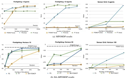
Each experiment was run for a given number ofsimulations, the number of samples used at each step to choose an action, and averaged over a number ofepisodes. We report undiscounted return with the standard error. Experiments were run on a single core of a 2.5 GHz machine with 8GB of memory. In both cases, we compare our factored representations to the flat version using POMCP. This comparison uses the same code base so it directly shows the difference when using factorization. POMCP and similar sample-based planning methods have already been shown to be state-of-the-art methods in both POMDP planning (Silver and Veness, 2010) and learning (Ross et al., 2011).

MPOMDPs. We start by comparing the factored statistics (FS) and factored tree (FT) versions of FV-POMCP

in multiagent planning problems. Here, the agents are given the true MPOMDP model (in the form of a simula-tor) and use it to plan. For this setting, we compare to two baseline methods:POMCP: regular POMCP applied to the MPOMDP, andrandom: uniform random action selection. Note that while POMCP will converge to an -optional solution, the solution quality may be poor when using small number of simulations.

1 100 500 1000 5000 10000 50000 75000 0 100 500 1000 5000 10000 50000 75000

POMCP (true) -85.97 -77.74 -42.53 -28.48 -21.16 -21.26 -20.6 0.948415 1.14661 2.35085 1.99687 0.79721 0.971969 0.853698

FS (true) -85.97 -37.44 -27.14 -26.66 -24.67 -24.65 -23.36 0.948415 2.01417 1.20706 1.25182 1.00768 0.934813 0.928388

FT (true) -85.97 -37.14 -37.7229 -37.3 -37.6 -36.91 -37.44 0.948415 1.42464 1.24872 1.25479 1.28973 1.23993 1.25142

Random -85.97 0.948415

Firefighting: 4 Agents

Value -90 -75 -60 -45 -30 -15

Number of Simulations

100 1000 10000 100000

POMCP (true) FS (true) FT (true) Random

1

Value -100 -93 -86 -79 -72 -65

Number of Simulations

100 1000 10000 100000

POMCP (true) FS (true) FT (true)

errors

1 100 500 1000 5000 10000 50000 0 100 500 1000 5000 10000 50000 0 100 500 1000 5000 10000 50000 0 100 500 1000 5000 10000 50000

POMCP (true) -99.5 -99.56 -98.97 -99.49 -99.51 -99.29 -99.18 0.140357 0.151208 0.25979 0.176349 0.178603 0.28576 0.227324 POMCP (true) -99.5 -99.56 -98.97 -99.49 -99.51 -99.29 -99.18 0.140357 0.151208 0.25979 0.176349 0.178603 0.28576 0.227324

FS (true) -99.5 -95.17 -84.24 -80.12 -70.65 -70.49 -68.66 0.140357 0.603062 1.46042 1.51964 1.08743 1.17197 1.14273 Factored statistics

(true)

-99.5 -97.46 -85.24 -80.64 -75.94 -75.64 -71.24 0.140357 0.603062 1.46042 1.51964 1.08743 1.17197 1.14273

FT (true) -99.5 -69.77 -67.37 -66.25 -67.7172 -66.19 -66.9 0.140357 1.52062 1.3457 1.29859 1.26737 1.76766 1.19686 Factored tree (true) -99.5 -74.51 -72.51 -72.31 -72.59 -76.2353 -75.7188 0.140357 1.52062 1.3457 1.29859 1.26737 1.76766 1.19686

Random -99.5 -99.5 -99.5 -99.5 -99.5 -99.5 -99.5 0.140357 0.140357 0.140357 0.140357 0.140357 0.140357 0.140357 Random -99.5 -99.5 -99.5 -99.5 -99.5 -99.5 -99.5 0.140357 0.140357 0.140357 0.140357 0.140357 0.140357 0.140357

FFG: Horizon 10

Value -100 -93 -86 -79 -72 -65

Number of Simulations

0 10000 20000 30000 40000 50000

POMCP (true) FS (true) FT (true) Random

Random

1

errors

0 100 1000 10000 0 100 1000 10000

POMCP (true) -5772.08 '5796.7 '5823.9 '5488.18 12.0325 41.0094 41.4847 70.783

FS (true) -5772.08 '5814.7 '4460.1 3907.14 12.0325 32.2606 101.214 46.4984

FT (true) -5772.08 '5785.9 '3220.85 '3181.92 12.0325 39.2071 53.393 105.117

Random -5772.08 -5772.08 -5772.08 -5772.08 12.0325 12.0325 12.0325 12.0325

Sensor Grid: 8 agents

Va lu e -6000 -4500 -3000 -1500 0 1500 3000 4500

Number of Simulations

100 1000 10000

POMCP (true) FS (true) FT (true) Random

1 (a) MPOMDP results

Firefighting: Horizon 10

Value -90 -74 -58 -42 -26 -10

Number of Simulations

0 125 250 375 500

FS FT BA-POMCP POMCP (true)

Random

9

Firefighting: Horizon 50

Value -500 -375 -250 -125 0

Number of Simulations

0 50 100 150 200 250

FS FT BA-POMCP

Random POMCP (true)

3

errors

0 50 100 500 1000 5000 0 50 100 500 1000 5000

POMCP (true) -1749 -1765.95 -1664.6 2715.05 36.3051

FS '1767.68 '1765.91 '1746.04 1127.31 4247.21 5752.47 10.6662 10.7417 10.9585 149.315 40.4285 51.1254

FT '1767.68 '1692.69 '611.47 '603.59 '593.521 '599.286 10.6662 11.3504 12.3876 20.5541 12.2871 153.548

BA-POMCP '1775.16 '1783.55 '1775.73 '1609.37 '682.32 4997.73 10.8695 10.7143 10.2748 12.0041 32.6295 41.4148

No learning '1775.16 '1783.55 '1779.22 '1610.55 '804.615 4667 10.8695 10.7143 10.3674 11.3882 28.5594 92.9594

Random '1767.68 '1767.68 '1767.68 '1767.68 '1767.68 POMCP1100001

sims err 7403.65 13.4053

Sensor Grid: Horizon 100

Va lu e -2000 -100 1800 3700 5600 7500

Number of Simulations

0 1000 2000 3000 4000 5000

FS FT BA-POMCP No learning

Random POMCP (true)

Sensor Grid: Horizon 100

Va lu e -2000 -100 1800 3700 5600 7500

Number of Simulations

0 200 400 600 800 1000

FS FT BA-POMCP

Random POMCP (true)

1 (b) BA-MPOMDP results

Figure 4: Results for (a) the planning (MPOMDP) case (log scale x-axis) and (b) the learning (BA-MPOMDP) case for the firefighting and sensor grid problems.

very well with a small number of samples and FS continues to improve until it reaches solution that is similar to FT.

Similar results are seen in the sensor grid problem. POMCP outperforms a random policy as the number of simulations grows, but FS and FT produce much higher values with the available simulations. FT seems to converge to a low quality solution (in both planning and learning) due to the loss of information about the target’s previous position that is no longer known to local factors. In this problem, POMCP requires over 10 minutes for an episode of 10000 simulations, making reducing the number of simulations crucial in problems of this size. These results clearly illustrate the benefit of FV-POMCP by exploiting structure for planning in MASs.

BA-MPOMDPs. We also investigate the learning setting (i.e., when the agents are only given the BA-POMDP

model). Here, at the end of each episode, both the state and count vectors are reset to their initial values. Learning in partially observable environments is extremely hard, and there may be many equivalence classes of transition and observation models that are indistinguishable when learning. Therefore, we assume a reasonably good model of the transitions (e.g., because the designer may have a good idea of the dynamics), but only a poor estimate of the observation model (because the sensors may be harder to model).

For the BRL setting, we compare to the following baseline methods: POMCP: regular POMCP applied to the true model using 100,000 simulations (this is the best proxy for, and we expect this to be very close to, the optimal value), andBA-POMCP: regular POMCP applied to the BA-POMDP.

Results for a four agent instance of the fire fighting problem are shown in Fig. 4(b), forh= 10,50. In both cases, the FS and FT variants approach the POMCP value. For a small number of simulations FT learns very quickly, providing significantly better values than the flat methods and better than FS for the increased horizon. FS learns more slowly, but the value is better as the number of simulations increases (as seen in the horizon 10 case) due to the use of the full history. After more simulations in the horizon 10 problem, the performance of the flat model (BA-MPOMDP) improves, but the factored methods still outperform it and this increase is less

visible for the longer horizon problem.

Similar results are again seen in the four agent sensor grid problem. FT performs the best with a small number of simulations, but as the number increases, FS outperforms other methods. Again, for these problems, BA-POMCP requires over 10 minutes for each episode for the largest number of simulations, showing the need for more efficient methods. These experiments show that even in challenging multiagent settings with state uncertainty, BRL methods can learn by effectively exploiting structure.

7

Related Work

MCTS methods have become very popular in games, a type of multiagent setting, but no action factorization has been exploited so far (Browne et al., 2012). Progressive widening (Coulom, 2007) and double progressive widening (Cou¨etoux et al., 2011) have had some success in games with large (or continuous) action spaces. The progressive widening methods do not use the structure of the coordination graph in order to generalize value over actions, but instead must find the correct joint action out of the exponentially many that are available (which may require many trajectories). They are also designed for fully observable scenarios, so they do not address the large observation space in MPOMDPs.

The factorization of the history in FTs is not unlike the use of linear function approximation for the state components in TD-Search (Silver, Sutton, and M¨uller, 2012). However, in contrast to that method, due to our particular factorization, we can still apply UCT to aggressively search down the most promising branches of the tree. While other methods based on Q-learning (Guestrin, Lagoudakis, and Parr, 2002; Kok and Vlassis, 2006) exploit action factorization, they assume agents observe individual rewards (rather than the global reward that we consider) and it is not clear how these could be incorporated in a UCT-style algorithm.

Locality of interaction has also been considered previously in decentralized POMDP methods (Oliehoek, 2012; Amato et al., 2013) in the form of factored Dec-POMDPs (Oliehoek, Whiteson, and Spaan, 2013; Pa-jarinen and Peltonen, 2011) and networked distributed POMDPs (ND-POMDPs) (Nair et al., 2005; Kumar and Zilberstein, 2009; Dibangoye et al., 2014). These models make strict assumptions about the information that the agents can use to choose actions (only the past history of individual actions and observations), thereby significantly lowering the resulting value (Oliehoek, Spaan, and Vlassis, 2008). ND-POMDPs also impose ad-ditional assumptions on the model (transition and observation independence and a factored reward function). The MPOMDP model, in contrast, does not impose these restrictions. Instead, in MPOMDPs, each agent knows thejointaction-observation history, so there are not different perspectives by different agents. Therefore, 1) factored Dec-POMDP and ND-POMDP methods do not apply to MPOMDPs; they specify mappings from individual histories to actions (rather than joint histories to joint actions), 2) ND-POMDP methods assume that the value function isexactlyfactored as the sum of local values (‘perfect locality of interaction’) while in an MPOMDP, the value is onlyapproximatelyfactored (since different components can correlate due to condition-ing the actions on central information). While perfect locality of interaction allows a natural factorization of the MPOMDP value function, but our method can be applied to any MPOMDP (i.e., given any factorization of the value function). Furthermore, current factored Dec-POMDP and ND-POMDP models generate solutions given the model in an offline fashion, while we consider online methods using a simulator in this paper.

8

Conclusions

We presented the first method to exploit multiagent structure to produce a scalable method for Monte Carlo tree search for POMDPs. This approach formalizes a team of agents as a multiagent POMDP, allowing planning and BRL techniques from the POMDP literature to be applied. However, since the number of joint actions and observations grows exponentially with the number of agents, na¨ıve extensions of single agent methods will not scale well. To combat this problem, we introduced FV-POMCP, an online planner based on POMCP (Silver and Veness, 2010) that exploits multiagent structure using two novel techniques—factored statistics and factored trees— to reduce 1) the number of joint actions and 2) the number of joint histories considered. Our empirical results demonstrate that FV-POMCP greatly increases scalability of online planning for MPOMDPs, solving problems with 10 agents. Further investigation also shows scalability to the much more complex learning problem with four agents. Our methods could also be used to solve POMDPs and BA-POMDPs with large action and observation spaces as well the recent Bayes-Adaptive extension (Ng et al., 2012) of the self interested I-POMDP model (Gmytrasiewicz and Doshi, 2005).

Acknowledgments

F.O. is funded by NWO Innovational Research Incentives Scheme Veni #639.021.336. C.A was supported by AFOSR MURI project #FA9550-09-1-0538 and ONR MURI project #N000141110688.

References

Amato, C., and Oliehoek, F. A. 2013. Bayesian reinforcement learning for multiagent systems with state uncertainty. InWorkshop on Multi-Agent Sequential Decision Making in Uncertain Domains, 76–83.

Amato, C.; Chowdhary, G.; Geramifard, A.; Ure, N. K.; and Kochenderfer, M. J. 2013. Decentralized control of partially observable Markov decision processes. InCDC, 2398–2405.

Amin, K.; Kearns, M.; and Syed, U. 2011. Graphical models for bandit problems. InUAI, 1–10.

Browne, C.; Powley, E. J.; Whitehouse, D.; Lucas, S. M.; Cowling, P. I.; Rohlfshagen, P.; Tavener, S.; Perez, D.; Samothrakis, S.; and Colton, S. 2012. A survey of Monte Carlo tree search methods.IEEE Trans. Comput. Intellig. and AI in Games4(1):1–43.

Cou¨etoux, A.; Hoock, J.-B.; Sokolovska, N.; Teytaud, O.; and Bonnard, N. 2011. Continuous upper confidence trees. InLearning and Intelligent Optimization. 433–445.

Coulom, R. 2007. Computing elo ratings of move patterns in the game of go. International Computer Games Association (ICGA) Journal30(4):198–208.

Dibangoye, J. S.; Amato, C.; Buffet, O.; and Charpillet, F. 2014. Exploiting separability in multi-agent planning with continuous-state MDPs. InAAMAS.

Fairbank, M., and Alonso, E. 2012. The divergence of reinforcement learning algorithms with value-iteration and function approximation. InInternational Joint Conference on Neural Networks, 1–8. IEEE.

Gmytrasiewicz, P. J., and Doshi, P. 2005. A framework for sequential planning in multi-agent settings. JAIR 24.

Guestrin, C.; Koller, D.; and Parr, R. 2001. Multiagent planning with factored MDPs. InNIPS, 15.

Guestrin, C.; Lagoudakis, M.; and Parr, R. 2002. Coordinated reinforcement learning. InICML, 227–234.

Kearns, M.; Mansour, Y.; and Ng, A. Y. 2002. A sparse sampling algorithm for near-optimal planning in large Markov decision processes.MLJ49(2-3).

Kok, J. R., and Vlassis, N. 2006. Collaborative multiagent reinforcement learning by payoff propagation.JMLR 7.

Kumar, A., and Zilberstein, S. 2009. Constraint-based dynamic programming for decentralized POMDPs with structured interactions. InAAMAS.

Messias, J. V.; Spaan, M.; and Lima, P. U. 2011. Efficient offline communication policies for factored multiagent POMDPs. InNIPS 24.

Nair, R.; Varakantham, P.; Tambe, M.; and Yokoo, M. 2005. Networked distributed POMDPs: a synthesis of distributed constraint optimization and POMDPs. InAAAI.

Ng, B.; Boakye, K.; Meyers, C.; and Wang, A. 2012. Bayes-adaptive interactive POMDPs. InAAAI.

Oliehoek, F. A.; Spaan, M. T. J.; Whiteson, S.; and Vlassis, N. 2008. Exploiting locality of interaction in factored Dec-POMDPs. InAAMAS.

Oliehoek, F. A.; Spaan, M. T. J.; and Vlassis, N. 2008. Optimal and approximate Q-value functions for decentralized POMDPs.JAIR32:289–353.

Oliehoek, F. A.; Whiteson, S.; and Spaan, M. T. J. 2012. Exploiting structure in cooperative Bayesian games. InUAI, 654–664.

Oliehoek, F. A.; Whiteson, S.; and Spaan, M. T. J. 2013. Approximate solutions for factored Dec-POMDPs with many agents. InAAMAS, 563–570.

Oliehoek, F. A. 2012. Decentralized POMDPs. In Wiering, M., and van Otterlo, M., eds.,Reinforcement Learning: State of the Art. Springer.

Pajarinen, J., and Peltonen, J. 2011. Efficient planning for factored infinite-horizon DEC-POMDPs. InIJCAI, 325–331.

Pynadath, D. V., and Tambe, M. 2002. The communicative multiagent team decision problem: Analyzing teamwork theories and models.JAIR16.

Ross, S.; Pineau, J.; Paquet, S.; and Chaib-draa, B. 2008. Online planning algorithms for POMDPs.JAIR32(1).

Ross, S.; Pineau, J.; Chaib-draa, B.; and Kreitmann, P. 2011. A Bayesian approach for learning and planning in partially observable Markov decision processes.JAIR12.

Silver, D., and Veness, J. 2010. Monte-carlo planning in large POMDPs. InNIPS 23.

Silver, D.; Sutton, R. S.; and M¨uller, M. 2012. Temporal-difference search in computer Go. MLJ87(2):183– 219.

Stone, P., and Sutton, R. S. 2001. Scaling reinforcement learning toward RoboCup soccer. InICML, 537–544.

Tesauro, G. 1995. Temporal difference learning and TD-Gammon.Commun. ACM38(3):58–68.

A

FV-POMCP Pseudo code

Algorithm 1POMCP

1: procedureSIMULATE(s,h,depth)

2: ifγdepth_{< then}

3: return0 .Stop when desired precision reached

4: end if

5: ifh6∈T then .if we did not visit thishyet

6: for alla∈Ado

7: T(h,a)←(Ninit(h,a),Vinit(h,a),∅) .initialize counts for alla, and particle filter

8: end for

9: returnRollout(s,h,depth) .do a random rollout from this node

10: end if

11: a←arg max0aQ(h,a0) +c

q_logN(h)

N(h,a0₎ .max via enumeration

12: (s0,o,r)∼ G(s,a) .sample a transition, observation and reward

13: R←r+γSimulate(s0,(hao),depth+ 1) .Recurse and receive the returnR

14: B(h)←B(h)∪ {s} .Addsto the particle filter maintained forh

15: N(h)←N(h) + 1 .Update the number of timeshis visited. . . 16: N(h,a)←N(h,a) + 1 .. . . and how often we selected actionahere 17: Q(h,a)←Q(h,a) +R_N−Q_(h,a(h,a₎) .Incremental update of mean return

18: returnR

19: end procedure

Algorithm 2Factored Statistics

1: procedureSIMULATE(s,~h,depth)

2: ifγdepth< then

3: return0

4: end if

5: if~h6∈T then

6: for all e∈E do .initialize statistics for componente

7: for all ~ae∈A~e do .only loop overlocaljoint actions

8: T(~h,~ae)←(Ninit(~h,~ae),Vinit(~h,~ae),∅)

9: end for

10: end for

11: returnRollout(s,~h,depth)

12: end if

13: ~a←arg max_~0_aP e

h

Qe(~h,~a0e) +c r

logN(~h+1)

n_~a0

e

i

.via variable elimination

14: (s0,~o,r)∼ G(s,~a)

15: R←r+γSimulate(s0,(~h~a~o),depth+ 1) 16: B(~h)←B(~h)∪ {s}

17: N(~h)←N(~h) + 1

18: for all~e∈Edo .update the statistics for each component

19: n~ae ←n~ae+ 1

20: Qe(~h,~ae)←Qe(~h,~ae) +R−Qe( ~ h,~ae)

n~ae .update the estimation of the expert for~ae

21: end for

22: returnR

23: end procedure

The pseudo code for the factored statistics case (FS-FV-POMCP) is shown in Algorithm 2. The comments highlight the important changes: there is no need to loop over the joint actions for initialization, or for selecting the maximizing action. Also, the same returnRis used to update the active expert in each componente.

Finally, Algorithm 3 shows the pseudo code for the factored trees variant of FV-POMCP. Like FSs, FT-FV-POMCP performs the simulations in lockstep. However, as we now maintain statistics and particle filters for each componentein separate trees, the initialization and updating of these statistics is slightly different. As such, the algorithm makes clear that there is no computational advantage to factored trees (when compared to FSs), but that the big difference is in the additional generalization it performs.

The actual planning could take place in a number of ways: one agent could be designated the planner, which would require this agent to broadcast the computed joint action. Alternatively, each agent can in parallel perform an identical planning process (by, in the case of randomized planning, syncing the random number generators). Then each agent will compute the same joint action and execute its component. An interesting direction of future work is whether the planning itself can be done more effectively by distributing the task over the agents.

Algorithm 3Factored Trees

1: procedureSIMULATE(s,~h,depth)

2: ifγdepth< then

3: return0

4: end if

5: for all e∈E do .check all componentse

6: if~he6∈Tethen .if there is no node for~hein the tree for componenteyet

7: for all ~ae∈A~e do .only loop overlocaljoint actions

8: Te(~he, ~ae)←(Ninit(~he, ~ae),Vinit(~he, ~ae),∅)

9: end for

10: end if

11: end for

12: returnRollout(s,~h,depth)

13: ~a←arg max_~0_aP e

h

Qe(~he, ~a0e) +c r

logN(~he+1)

n_~a0

e

i

.via variable elimination

14: (s0,~o,r)∼ G(s,~a)

15: R←r+γSimulate(s0,(~h~a~o),depth+ 1)

16: for all~e∈Edo .update the statisitics for each component

17: B(~he)←B(~he)∪ {s} .update the particle filter of each treeewith the sames

18: N(~he)←N(~he) + 1

19: n~ae ←n~ae+ 1

20: Qe(~he, ~ae)←Qe(~he, ~ae) +R−Qe( ~_h

e,~ae)

n~ae .update expert for~he, ~ae

21: end for

22: returnR

23: end procedure

B

Analysis of Mixture of Experts Optimization

Here we analyze the behavior of our mixtures of experts under sample policy~π. In performing this analysis we compare to the case where the true value functionQ(~a)is factored inEcomponents

Q(~a) =

E X

e=1

Qe(~ae)

is the set of other componentse0which have an overlap withe: those that have at least one agent participating in them that also participates ine). In this analysis, we will assume that all experts are weighted uniformly (αe=_E1), and ignore this constant which is not relevant for determining the maximizing action.

Theorem 4. The estimateQˆ ofQmade by a mixture of experts converges in probability to the true value plus

a sample policy dependent bias term:

ˆ

Q(~a)→p Q(~a) +B~π(~a).

The bias is given by a sum of biases induced by pairse,e0of overlapping value components:

B~π(~a), X

e X

e0_6=e

X

~ a_e0 \e

~π(~ae0_\e|~ae)Qe0(~a_e0_\e,~ae0_∩e).

Here~ae0_∩eis the action of the agents that participate both ineande0(specified by~a) and~a_e0_\eare the actions

of agents ine0that are not ine(these are summed over as emphasised by the overlining).

Proof. Suppose that we have drawn a set of samplesr1, . . . ,rKaccording to~π. For each componenteand~ae,

we have an expert that estimatesQˆ(~ae). LetR(~ae)be the subset of samples received where we took local joint

action~ae. The corresponding expert will estimate

ˆ

Q(~ae) :=

1

R(~ae) X

r~ae∈R(~ae)

r~ae

Now, the expected sample that this expert receives is

E[r~ae|~π] = Eν





 X

~ a−e

~π(~a−e|~ae)Q(~a) +ν 





= X

~a−e

~

π(~a−e|~ae) "

X

e0

Qe0(~a_e0)

#

+Eνν

= Qe(~ae) + X

~a−e

~π(~a−e|~ae) X

e0_6=e

Qe0(~a_e0) + 0

= Qe(~ae) + X

e0_6=e

X

~a_{e0 \e}

~

π(~ae0_\e|~a_e)Q_e0(~a_e0_\e,~a_e0_∩e)

which means that the estimate of an expert converges in probability to a biased estimate

ˆ

Q(~ae) p

→Qe(~ae) +

X

e0_6=e

X

~a_e0 \e

~

π(~ae0_\e|~a_e)Q_e0(~a_e0_\e,~a_e0_∩e).

This, in turn means that the mixture of experts

ˆ

Q(~a) =X

e

ˆ

Qe(~ae) p

→X

e 



Qe(~ae) +

X

e0_6=e

X

~a_e0 \e

~

π(~ae0_\e|~ae)Qe0(~a_e0_\e,~ae0_∩e)



 

=X

e

Qe(~ae) + X

e X

e0_6=e

X

~a_e0 \e

~

π(~ae0_\e|~a_e)Q_e0(~a_e0_\e,~a_e0_∩e)

=X

e

Qe(~ae) +B~π(~a),

as claimed.

As is clear from the definition of the bias term, it is caused by correlations in the sample policy and the fact that we are over counting value from other components. When there is no overlap in the payoff components, and we use a sample policy we use is ‘component-wise’, i.e.,~π(~ae0_\e|~a_e) =~π(~a_e0_\e|~a0_e) =π~(~a_e0_\e), the effect

of this bias can be disregarded: in such a case, even though all componentse0 6= econtribute to the bias of expertethis bias is constant for those componentse0 6∈ N(e). Since we care only about the relative values of joint actions~a, only overlapping components actually contribute to introducing error. This is clearly illustrated for the case where there are no overlapping components.

Theorem 5. In the case that the value components do not overlap, mixture of experts optimization recovers the

maximizing joint action.

Proof. In this case,

ˆ

Qe(~ae) p

→Qe(~ae) +

X

e0_6=e

X

~ ae0

~

πe0(~a_e0)Q_e0(~a_e0)

and the bias does not depend on~ae, such that

arg max

~ae

ˆ

Qe(~ae) p

→arg max

~ae

Qe(~ae) +C= arg max ~ae

Qe(~ae).

And for the joint optimization:

ˆ

Q(~a) =X

e

ˆ

Qe(~ae) p

→X

e 

Qe(~ae) + X

e0_6=e

X

~a_e0

~

πe0(~a_e0)Q_e0(~a_e0)





=X

e

Qe(~ae) + X

e X

e0_6=e

X

~a_e0

~πe0(~a_e0)Q_e0(~a_e0)

=X

e

Qe(~ae) + (E−1) X

e X

~a0

e

~

πe(~a0e)Qe(~a0e)

=X

e

(Qe(~ae) + (E−1)SA(e,~π))

whereSA(e,~π) =P ~a0

e~πe(~a

0

e)Qe(~a0e)is the sampled average payoff of componentewhich affects our value

estimates, but which does not affect the maximizing joint action:

arg max

~a "

X

e

(Qe(~ae) + (E−1)SA(e,~π)) #

= arg max

~ a

X

e

Qe(~ae)

Similar reasoning can be used to establish bounds on the performance of mixture of expert optimization in cases with overlap, as is shown by the next theorem.

Theorem 6. If for all overlapping componentse,e0, and any two ‘intersection action profiles’~ae0_∩e,~a0_e0_∩efor

their intersection, the true value function satisfies that

∀~ae0_\e Q_e0(~a_e0_\e,~a_e0_∩e)−Q_e0(~a_e0_\e,~a0_e0_∩e)≤

E· |N(e)| ·

~

Ae0_\e

·~π(~ae0\e)

, with ~

Ae0_\e

the number of intersection action profiles, then mixture of experts optimization, in the limit will

Proof. Bias by itself is no problem, but different bias for different joint actions is, because that may cause us to select the wrong action. As such, we set out to bound

∀~a,~a0 |B_~π(~a)−B_~π(~a0)| ≤.

As explained, only terms where the bias is different for two actions~a,~a0matter. As such we will omit terms that cancel out. In particular, we have that if two componentse,e0do not overlap, the expression

X

~a_{e0 \e}

~

π(~ae0_\e|~a_e)Q_e0(~a_e0_\e,~a_e0_∩e)−

X

~ a_{e0 \e}

~π(~ae0_\e|~a0_e)Q_e0(~a_e0_\e,~a0_e0_∩e)

reduces toP

~ae0~π(~ae0|~ae)Qe0(~ae0)−

P

~ae0~π(~ae0|~a 0

e)Qe0(~a_e0)and hence vanishes under a componentwise

pol-icy. We use this insight to define the bias in terms of neighborhood bias. Let us writeN(e)for the set of edges{e0}that have overlap withe, and let’s write~aN(e)for the joint action that specifies actions for that entire

overlap, then we can write this as:

B~π(~a), E X

e=1

B~πe(~aN(e))

with

B_~πe(~aN(e)) =

X

e0_∈N(e)

B_~e_π0∩e(~ae0_∩e)

componente’s ‘neighborhood bias’, with

B_~πe0→e(~ae), X

~a_e0 \e

~

π(~ae0_\e|~a_e)Q_e0(~a_e0_\e,~a_e0_∩e)

the ‘intersection bias’: the bias introduced onevia the overlap betweene0ande.

Now, we show how we can guarantee that the bias is small, by guaranteeing that the intersection biases are small. This gives a conservative bound, since different biases may very well cancel out. Artbitrarily select two actions, W.l.o.g. we select~ato be the larger-biased joint action. We need to guarantee that

B~π(~a)−B~π(~a0)≤

↔ E X

e=1

X

e0_∈N(e)

B_~πe0→e(~ae)− E X

e=1

X

e0_∈N(e)

B_~πe0→e(~a0_e)≤

↔ E X

e=1



 X

e0_∈N(e)

B_~πe0→e(~ae)− X

e0_∈N(e)

B_~πe0→e(~a0_e)



≤

← X

e0_∈N(e)

B_~πe0→e(~ae)− X

e0_∈N(e)

B_~πe0→e(~a0_e)≤

E ∀e

↔ X

e0_∈N(e)

h

B_~πe0→e(~ae)−Be

0_→e

~π (~a

0

e) i

≤

E ∀e

← hBe_~π0→e(~ae)−Be

0_→e

~

π (~a

0

e) i

≤

E× |N(e)| ∀e,e

0

let0 _,E×|N(e)|, we want

h

B~πe0→e(~ae)−Be

0_→e

~ π (~a0e)

i

≤0

X

~a_e0 \e

~

π(~ae0_\e|~a_e)Q_e0(~a_e0_\e,~a_e0_∩e)−

X

~ a_e0 \e

~π(~ae0_\e|~a0_e)Q_e0(~a_e0_\e,~a0_e0_∩e)≤0

↔ X

~a_{e0 \e}

~π(~ae0_\e|~a_e)Q_e0(~a_e0_\e,~a_e0_∩e)−~π(~a_e0_\e|~a0_e)Q_e0(~a_e0_\e,~a0_e0_∩e)

≤0

← ~π(~ae0_\e|~a_e)Q_e0(~a_e0_\e,~a_e0_∩e)−~π(~a_e0_\e|~a0_e)Q_e0(~a_e0_\e,~a0_e0_∩e)≤

0

~

Ae0_\e

∀_~a

e0 \e

Under a component-wise policy~π(~ae0_\e|~a_e) =~π(~a_e0_\e|~a0_e) =~π(~a_e0_\e)and thus

~

π(~ae0_\e)Qe0(~a_e0_\e,~ae0_∩e)−Q_e0(~a_e0_\e,~a0_e0_∩e)

≤

0

~

Ae0_\e

∀_~a

e0 \e

↔ Qe0(~a_e0_\e,~a_e0_∩e)−Q_e0(~a_e0_\e,~a0_e0_∩e)≤

0

~

Ae0_\e

~π(~ae0\e) ∀_~a

e0 \e

Putting it all together, if the factorized Q function satisfies that, for all the component intersections, the following holds:

∀~ae0_\e,~a_e0_∩e,~a0_e0_∩e Qe0(~a_e0_\e,~a_e0_∩e)−Q_e0(~a_e0_\e,~a0_e0_∩e)≤

E|N(e)|

~

Ae0_\e

~π(~ae0\e)