Three-dimensional image classification using hierarchical spatial decomposition: A study using retinal data

(1)

Three-dimensional Image Classification Using

Hierarchical Spatial Decomposition: A Study

Using Retinal Data

Thesis submitted in accordance with the requirements of the University of Liverpool for the degree of Doctor in Philosophy

by

Abdulrahman Abdulaziz A Albarrak

(2)

Abstract

(3)

Acknowledgements

Of all the fantastic and fabulous people involved, I would like to express my deepest gratitude to my first supervisor, Prof. Frans Coenen, who has been abundantly helpful and has offered invaluable assistance, support, caring, patience, and guidance through-out my Ph.D. It is my privilege to have worked with him. Deepest gratitude is also due to my second supervisor, Dr. Yalin Zheng, without whose knowledge and assistance this research would not have been successful.

I would like to express my deepest gratitude to my family. They were always supporting me and encouraging me with their best wishes.

Special thanks also go to my colleague, Mr. Nattapon Boonarpha, for his collabora-tive research work and his scanning of the images. Special thanks also to all the staff in the Department of Computer Science at The University of Liverpool and the St. Paul’s Eye Unit at the Royal Liverpool University Hospital who have been helpful whenever needed. Not forgetting my fellow colleagues in Room 2.11 who always encouraged each other either directly or indirectly; my prayers go to all of you to succeed in everything that you do.

(4)

List of Figures

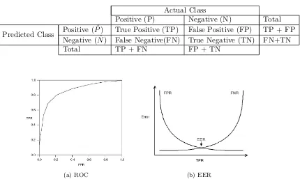
2.1 Forms of grid decomposition. . . 20 2.2 A diagram showing an example plot of ROC and EER. . . 29 2.3 The statistical differences and confidence intervals for the example results

in Table 2.4. . . 34

3.1 Section of human eye [76]. . . 36 3.2 A schematic of the retinal layers and the fovea [113]. . . 37 3.3 Illustration of the difference between (a) normal and AMD vision, (b)

a normal and an AMD eye (drusen present in the macula) and (c) a normal retina and an AMD retina [16]. . . 38 3.4 An example of an OCT scanner system, where CCD is the

Charge-Coupled Device [22]. . . 39 3.5 An OCT image showing different retinal layers [39]. . . 40 3.6 Examples of 3D OCT images from the RLUH data set used in this thesis

showing the difference between a “normal” and an AMD retina. . . 42 3.7 Examples of 3D OCT image before and after applying the preprocessing. 46 3.8 Examples of a set of slices for Figure 3.7. . . 47

4.1 Example of a 3D OCT volume showing the size in 3 dimensions (140 (x) ×140 (y) ×20(z) ). . . 49 4.2 Illustration of the effect of the seven different critical functions considered

in this thesis when applied to decompose the volume in Figure 4.1. . . 55 4.3 Standard volumetric decomposition versus the overlapping volumetric

decomposition. . . 56

5.1 Overview of the region-based classification process. . . 59 5.2 Example of a region (S), where the colour represents the intensity value. 61 5.3 Illustration of neighbours and directions of a voxel in a 3D region [18]. 63 5.4 Example of gradients with respect to the region presented in Figure 5.2. 69

(9)

6.2 Significance differences and confidence intervals for comparing levels of decomposition . . . 86 6.3 Confidence intervals for overlapping with standard decomposition. . . . 87 6.4 Significance differences and Confidence intervals for comparing

represen-tation techniques. . . 90 6.5 Confidence intervals for comparing single feature vector generation

tech-niques. . . 94 6.6 Confidence intervals for comparing different dictionary sizes K when

using IFK single feature vector generation. . . 94 6.7 Significance differences and confidence intervals for comparing classifiers. 96

7.1 Schematic illustrating the whole image-based representation approach to image classification. . . 100 7.2 Significance difference and confidence intervals for comparing critical

functions . . . 112 7.3 Confidence interval diagrams for comparing levels of decomposition (L=

{3,4,5,6}) . . . 113

(10)

List of Tables

2.1 Terminology used throughout this thesis . . . 12

2.2 Basic notation used throughout this thesis . . . 12

2.3 Confusion matrix . . . 29

2.4 Example accuracy classification results where there is statistical differ-ence in the operation of the classifiers. . . 33

2.5 Example accuracy classification results where there is not a statistical difference in the operation of the classifiers. . . 33

2.6 ANOVA results for the example results in Table 2.4. . . 33

2.7 ANOVA results for the example results in Table 2.5. . . 33

5.1 Symbols used for FOR . . . 60

5.2 FOR values for the region presented in Figure 5.2. . . 62

5.3 The possible 26 displacement vectors that can be associated with a voxel [18]. . . 63

5.4 Illustration of how to generate a GLCM from a region (d= 1 and Φ = 0). In the region, there are 3 intensity values (1,2, and 3). . . 64

5.5 Symbols used for VCM . . . 64

5.6 SOR values for the region presented in Figure 5.2 generated using a VCM 66 5.7 Illustration of how to generate a GLRLM from a region. In the region, there are three intensity values (1,2, and 3), the GLRLM for Φ = 0. . . 66

5.8 Symbols used for VRLM. . . 67

5.9 SOR values for the region presented in Figure 5.2 generated using a VRLM . . . 68

5.10 Example values for 8 bins generated using HOG with respect to the region presented in Figure 5.2. . . 69

5.11 Illustration of how to generate a CSLBP from a region. In the region, there are three intensity values (1,2, and 3). . . 70

5.12 Example values of eight bins generated using CSLBP with respect to the region presented in Figure 5.2. . . 71

5.13 Example values of eight bins generated using HOG-LBP with respect to the region presented in Figure 5.2. . . 71

(11)

5.15 Illustration of how to generate a LPQ for a region. In the region, there

are three intensity values (1, 2 and 3). . . 72

5.16 Example values for eight bins generated by LPQ for the region in Figure 5.2. . . 72

6.3 The number of occasions when the best recorded AUC value from Ta-bles 6.1 and 6.2 with respect to level of decomposition L and type of decomposition (standard or overlapping) was recorded . . . 80

6.1 Classifier performance results using standard decomposition, the HOG region-based representation, dimensionality reduction using PCA and SVM classification in the context of decomposition (Stage 1) using: (i) a range of decomposition levels, (ii) a number of critical functions (in-cluding no critical function). . . 81

6.2 Classifier performance results using overlapping decomposition, the HOG region-based representation, dimensionality reduction using PCA and SVM classification in the context of decomposition (Stage 1) using: (i) a range of decomposition levels, (ii) a number of critical functions (in-cluding no critical function). . . 82

6.4 ANOVA table for comparing critical functions . . . 85

6.5 ANOVA table for comparing levels of decomposition . . . 86

6.6 Comparison of decomposition techniques . . . 86

6.7 Classifier performance results using overlapping decomposition, an ED critical function, dimensionality reduction using PCA and SVM classifi-cation in the context of region representation methods (Stage 2) using: (i)) a range of decomposition levels (L), (ii) the seven region-based rep-resentation techniques. . . 89

6.8 Comparison of region-based representation methods. . . 90

6.9 Classifier performance results using overlapping decomposition, a LCS critical function, the HOG region-based representation and ) SVM classi-fication in the context of single feature vector generation (Stage 3) using: (i) a range of decomposition levels (L), (ii) PCA and IFK (withK = 32) feature selection. . . 92

6.10 Classifier performance results using overlapping decomposition, a LCS critical function, the HOG region-based representation and (v) SVM classification in the context of the IFK single feature generation method with (i) a range of dictionary sizes and (ii) a range of decomposition levels. 92 6.11 Comparing IFK and PCA-based methods. . . 93

(12)

6.13 Classification results using a LCS critical functions, the HOG region-based representation, IFK feature selection (withK= 32) in the context of classifier generation (Stage 4) using: (i) a range of decomposition levels (L), (ii) three classifier generators (SVM, NB and KNN). . . 96 6.14 Comparing classifiers. . . 96 6.15 Best four performing combinations of techniques as identified in the

fore-going evaluation. . . 98 6.16 Summary of evaluation results obtained using the four best techniques

identified in Table 6.15 . . . 98

7.1 Classifier performance results in the context of decomposition (Stage 1) using: (i) standard decomposition with decomposition threshold t= 0.5, (ii) a range of decomposition levels (L), (iii) a number of critical functions, (iv) Kurtosis node labelling and (v) SVM classification. . . . 109 7.2 Classifier performance results in the context of decomposition (Stage

1) using: (i) overlapping decomposition with decomposition threshold

t= 0.5, (ii) a range of decomposition levels (L), (iii) a number of critical functions, (iv) Kurtosis node labelling and (v) SVM classification. . . . 110 7.3 The number of occasions when the best recorded AUC value from Tables

7.1 and 7.2 was recorded with respect to level of decomposition L and type of decomposition (standard or overlapping). . . 110 7.4 ANOVA data for critical function comparison . . . 111 7.5 ANOVA data for levels of decomposition comparison (L={3,4,5,6}) . 112 7.6 ANOVA data for decomposition comparison (standard v. overlapping) . 112 7.7 Classifier performance results in the context of the edge labelling

mech-anism used (Stage 2) using: (i) standard decomposition, (ii) a range of decomposition levels, (iii) KLD critical function, (iv) gSpan FSG using

σ= 2 and (v) SVM classification. . . 114 7.8 ANOVA data for edge-labelling comparison (Kurtosis v. Mean) . . . 115 7.9 Classifier performance results in the context of classifiers generation

(Stage 5) using: (i) standard decomposition, (ii) a range of decompo-sition levels, (iii) KLD critical function and (iv) Kurtosis node labelling. 116 7.10 ANOVA data for classifier generation comparison. . . 117 7.11 Best four performing combinations of techniques as identified in the

fore-going evaluation. . . 118 7.12 The best classification results obtained using decomposition and whole

image-based methods. . . 118

(13)

8.2 Best four performing combinations of techniques for whole image-based

methods. . . 121

8.3 Best classification results for the alternative techniques, RB techniques, WIB techniques. . . 123

8.4 The average run time in seconds for the identified methods in this chap-ter. The following are given: Average Decomposition Time (ADT), Av-erage Feature Vector Generation Time (AFVGT), Classifier Generation (CG) and Total Execution Time (TET). . . 124

A.1 The results using FOR with PCA. . . 132

A.2 The results using VCM with PCA. . . 136

A.3 The results using VRLM with PCA. . . 140

A.4 The results using HOG with PCA. . . 144

A.5 The results using LBP with PCA. . . 148

A.6 The results using HOG-LBP with PCA. . . 152

A.7 The results using LPQ with PCA. . . 156

A.8 IFK results without using a critical function (0NCF). . . 160

A.9 The results of using the AIV critical function in the context of IFK. . . 163

A.10 The results of using the GLCM critical function using IFK. . . 165

A.11 The results of using the KCC critical function using IFK. . . 167

A.12 The results of using the ED critical function using IFK. . . 170

A.13 The results of using the DTW critical function using IFK. . . 172

A.14 The results of using the LCS critical function using IFK. . . 175

A.15 The results of using the KLD critical function using IFK. . . 177

B.1 The results using the AIV critical function in the context of whole image-based methods, where S means standard decomposition, O overlapped decomposition, t is the threshold for the critical function and L is the level. . . 182

B.2 The results using the ED critical function in the context of whole image-based methods, where S means standard decomposition, O overlapped decomposition, t is the threshold for the critical function and L is the level.. . . 186

B.3 The results using the KCC in the context of whole image-based methods, where S means standard decomposition, O overlapped decomposition, t is the threshold for the critical function and L is the level.. . . 190

(14)

(15)

List of Algorithms

4.1 Pseudocode for the proposed hierarchical spatial decomposition method 50 7.1 Pseudocode for the tree labelling. . . 101 7.2 Pseudocode for the proposed feature vector generation for the whole

(16)

Notation

The following notations and abbreviations are found throughout this thesis:

2DTwo Dimensional.

3DThree Dimensional.

AMDAge-related Macular Degeneration.

ANOVAAnalysis Of Variance.

AUCArea Under the receiver operating Curve.

DM Data Mining.

DLDictionary Learning.

FSMFrequent Sub-tree Mining.

IMImage Mining.

k-NNk-Nearest Neighbour.

KDDKnowledge Discovery in Databases.

KDI Knowledge Discovery in Images.

NBNaive Bayes classifier.

RBRegion-Based.

SVMSupport Vector Machine.

TCVTen-fold Cross Validation.

VOIVolume Of Interest.

(17)

Chapter 1

Introduction

1.1 Overview

The past decade has seen the rapid development of three-dimensional (3D) imaging acquisition technologies. This recent innovation has highlighted the need for more advanced techniques to analyse such 3D image data. The potential for such techniques is further highlighted by progress in the amount of computational power and storage that is now available. There are a number of application domains where 3D images are regularly used. One important domain is the medical domain where many different types of images are used to support the prediction and management of diseases and conditions.

Knowledge Discovery in Databases (KDD), or simply Knowledge Discovering in Data, is a computer science technology directed at turning low-level data into high-level knowledge [46]. More formally KDD can be described as the non-trivial process of identifying valid, novel, potentially useful, previously unknown, and ultimately under-standable patterns and useful information from data. The data mining element of the KDD process can be argued to be the most significant element of the entire process; it is where the desired knowledge discovery is actually undertaken. Data mining is thus concerned with the specific task of extracting hidden patterns and/or other useful information from the input data. Various techniques, from various disciplines, have been proposed with which to conduct the data mining [36].

(18)

One common image mining task is image classification. Classification can be defined as the process of automatically creating a piece of software, called a classifier, which can be used to categorise unseen data. Classifiers are typically built using a pre-labelled

training set and their effectiveness is typically established by applying it to a test set

whose labels are known (thus the actual labels can be compared with the derived labels). In the case of image classification, a classifier might be built for the purpose of disease/no-disease categorisation of medical images (“normal” versus “abnormal”). This type of image classification is known as whole-image classification in contrast to other types of classification where the task is to base the classification on some object contained within an image.

Image mining is typically directed at two-dimensional (2D) images; however, as noted above, recent technology exists whereby we can acquire 3D images (volumes). Volumetric 3D image mining has received much less attention than 2D image mining [6, 104, 149, 142]. This is largely because 3D image mining is a much more resource intensive task than 2D image mining. In the context of image classification 3D image classification is therefore a challenging task. However, 3D image classification provides a solution to the need for advanced techniques with which to analyse 3D image data as noted at the start of this section.

The subject matter for this thesis is thus 3D (volumetric) medical image classifi-cation. The main issue with 3D image classification is not so much the data mining techniques to be applied, these are frequently well understood, but the preprocessing of the 3D data so as to enable the application of data mining techniques. The challenge here is to translate the input data into some appropriate representation compatible with the data mining techniques to be adapted, while at the same time ensuring that no key elements are lost, elements that may be significant with respect to effective 3D image classification. This thesis proposes a number of approaches to deal with the problem of 3D image classification founded on the idea of hierarchical spatial decomposition. The justification for this is presented in Section 1.3 below. Note that we can identify two broad mechanisms for using 3D hierarchical decomposition in the context of 3D volume classification. We can represent the decomposition using regions identified in the decomposition (region-based) or we can represent the entire decomposition (whole image-based).

To act as a focus for the research, the work has been directed at the detection of retinal diseases such as Age-related Macular Degeneration (AMD) in 3D volumes produced using Optical Coherence Tomography (OCT). Analogous to ultrasound, OCT is a relatively new imaging technology that can produce cross-sectional views of a retina at a high level of resolution and speed. AMD is a condition typically contracted in old age, which leads to irreversible vision loss at its advanced stages [21, 66].

(19)

dis-cussion concerning the motivation for the work is presented in Section 1.2. The specific “research question”, and associated research issues, are presented in Section 1.3. Sec-tion 1.4 outlines the research methodology adopted to address the research quesSec-tion and issues, including the adopted evaluation strategy. Section 1.5 then highlights the research contribution of the work, and Section 1.6 presents some of the published work resulting from the research presented in this thesis. Section 1.7 reviews the structure of the rest of this thesis.

1.2 Motivations

The main aim of the investigation presented in this thesis is to find efficient and ac-curate approaches to represent 3D images using the concept of hierarchical spatial decomposition, which will enable reliable classification with respect to real-world prob-lems. Most of the research on volumetric date analysis to date has tended to focus on feature extraction [32, 129, 139], image segmentation [55, 58, 136] and image alignment and registration [93] rather than classification. There is very little published work on the classification of volumetric data [1, 127]. In practice, at least with respect to the medical image mining domain, this tends to be done by hand; although there are vari-ous tools in current use to support 3D image analysis and diagnosis, these tend not to fully automate the process. The automated diagnosis of diseases using 3D data, even if only coarsely achieved, would clearly ease the time resource required to process such images. Areas where automated diagnosis would be of particular value are in screen-ing programmes where large quantities of image data need to be processed in such a way that patients can receive results during the same consultation in which the data is acquired (point of care diagnosis). Examples include breast and prostrate cancer screening, although this is usually done using 2D images. In the case of 3D volumetric imaging, the problem is more acute as there is much more data to consider; 3D data sets tend to be an order of magnitude larger than 2D data sets. One type of screening programme where 3D images are regularly used are retina screening programmes. For example, screening programmes for the detection of AMD are currently under consid-eration given the global ageing population. Another example is screening programs for diabetics who are frequently screened for diabetic retinopathy using 3D retinal images. In the medical domain there are a number of technologies typically used to generate 3D volumes; these include: Cone Beam Computed Tomography (CBCT), Magnetic Resonance Imagery (MRI) and Optical Coherence Tomography (OCT). The focus of the research is thus the detection of AMD in 3D OCT. The motivations for choosing this application domain as a “driver” for the research described in this thesis are as follows:

(20)

mining applied to 3D OCT image data, although there have been a number of reported studies with respect to macular disease diagnosis using 2D OCT images [49, 88]. Most reported work on OCT image analysis is directed at retinal layer segmentation [70, 150], vessel segmentation [71], image enhancement [81] and noise reduction [110].

2. With the increasing widespread use of 3D OCT techniques many clinicians have found that they are “overwhelmed” by the quantity of data available for analysis. They are limited by time and resources. There is also a lack of automated diag-nosis tools; most existing tools are directed at supporting the analysis, such as tools for retinal thickness measurement. In practice, subjective assessment is the mainstay. Although the clinicians do an outstanding job the process is subject to human error and skill. Therefore, automated diagnosis tools, founded on the technology proposed in this thesis, are desirable; not only to provide for better patient management but also to provide for staff training.

3. More generally, Computer-Aided Diagnosis (CAD) is an important element of many branches of medical care, not just in the case of 3D retinal diagnosis. Gen-erally applicable approaches to support automate CAD are therefore desirable.

4. Intuitively, for many medical applications (including retinal image diagnosis), being able to use 3D data sets to support the diagnosis is likely to be much more effective than when using 2D data sets. It is anticipated that volumetric data is likely to reveal more information about the scanned objects than 2D data.

1.3 Research Questions and Issues

Given the research motivation presented in Section 1.2 above the work described in this thesis is targeted at an investigation of techniques to facilitate the diagnosis of 3D medical images. More specifically, the work is directed at the development of various ways to represent 3D volumes so that efficient and effective 3D classifiers can be generated using hierarchical spatial decomposition techniques to represent 3D images for classification. Thus the overarching research question addressed by this thesis is:

Is it possible to devise hierarchical spatial decomposition-based

represen-tation methods, suited to the classification of volumetric data, in such a way

that effective classification performance can be achieved given the significant

size and complexity of volumetric data sets?

The reasons for adapting a decomposition approach are as follows:

(21)

context of data mining the patterns we are interested in generally tend to be a description or a model of a subset of the data [35].

• Hierarchical decomposition allows for a more “complete” analysis in that the

analysis can be directed at different levels of the decomposition.

• There is evidence to suggest that image representation methods that rely on localised features tend to produce better performance than those that use global features. Examples of such localised methods include: (i) Scale-Invariant Feature Transform (SIFT) [90, 91, 92], (ii) Histograms of Oriented Gradients (HOGs) [25], and (iii) Local Binary Patterns (LBPs) [98] and their extension to 3D [40, 119, 123, 157].

• Hierarchical decomposition analysis allows for the identification of regions with similar (homogeneous) properties, properties that may be significant with respect to classification of the volume under consideration.

• Spatial relationships between regions can be maintained. Regions that share the

same parent remain identifiable.

• Once the decomposition has been established it can be used in a variety of different

ways; in other words, decomposition is a versatile technique. Principally we can choose to represent the decomposition in its entirety (whole image-based) or we can consider individual regions within the decomposition in isolation (region-based).

A central issue with respect to representations that are founded on the concept of hierarchical spatial decomposition is the termination condition for the decomposition (the so called “critical function”). Critical functions normally operate according to the “homogeneity” of individual regions. A further issue is the “overlap problem” where a particular object of interest is held in different parts of the decomposition; the object of interest overlaps several identified regions. The research presented in this thesis investigates various techniques to decompose the image by considering different approaches to ensure the homogeneity of the decomposed regions.

The above research question thus encompasses five subsidiary research questions:

1. What is the most appropriate method to decompose images? A number of different mechanisms for decomposing volumes can be identified although prior to the research described in this thesis it was unclear as to which was the most appropriate.

(22)

or in terms of the entire decomposition (whole image-based)? This is the most significant subsidiary research question, whose resolution is central to the work described in this thesis.

3. With respect to the use of either region-based or whole image-based representation, what is the most appropriate representation for encap-sulating the decomposition to support the desired classification? The issue here is that some image representation techniques result in a more classifi-cation effective representation than others.

4. Given a particular representation what is the most effective way of gen-erating a single feature vector for each image? Most classifier generation mechanisms ultimately operate using a feature vector representation. Thus re-gardless of what decomposition representation is adapted it needs to be eventually translatable into a feature vector form. The best process for this is unclear.

5. What is the most appropriate mechanism for conducting volumetric classification? Different image representations, even when features are trans-lated into a feature vector representation, will be compatible with different classi-fication techniques; however, it is unclear what the most appropriate technique for each representation is with respect to the representation proposed in this thesis.

1.4 Research Methodology

To provide answers to the above central research question posed by this thesis, and the subsidiary questions, the adapted research methodology was broadly to consider and evaluate a number of hierarchical spatial decomposition techniques, each operating in a different manner.

(23)

in some form of feature vector representation as this is the standard input format for most classifier generators (as noted above). Because ultimately a feature vector representation would need to be derived, feature selection and generation strategies were considered.

What ever the case the generated feature vectors could then be fed into a classifier generator, for which purpose a number of different classifier generators were considered and evaluated. The process of generating a classifier thus comprises different stages and at each stage there are different techniques that can be used. Therefore the evaluation of each stage was conducted by considering the proposed techniques for the stage in question while using a fixed set of techniques for the remaining stages. For each stage two types of evaluation were conducted: (i) individual performance evaluation, and (ii) statistical significance testing. Ten-fold Cross Validation (TCV) was used, whereby the image data set is randomly divided into ten sub-sets (each with the same number of images for each class). Each technique was then tested ten times, on each occasion with a different tenth as the test set. TCV is a well-established technique with respect to determining the effectiveness of classifiers. On each iteration the following was recorded: (i) accuracy, (ii) sensitivity, (iii) specificity, (iv) Positive Predictive Value (PPV), (v) Negative Predictive Value (NPV), (vi) Area Under the receiver operator characteristic Curve (AUC) and (vii) Equal Error Rate (EER). For the second type of evaluation, the ANalysis Of VAriance (ANOVA) statistical significance test was used.

1.5 Contributions

This thesis makes a number of contributions and these are summarised in this section. Firstly, the work demonstrates that it is possible to improve the performance of 3D image classification by adapting hierarchical spatial decomposition based representa-tion methods. It is argued that by decomposing regions down to homogeneous regions, it is possible to produce effective solutions to the 3D classification problem (various ways to extract homogeneous regions are introduced in this thesis). By hierarchical spatial decomposition, the multi-scale aspects of an image can further be characterised by considering a representation such as the tree-based representation where tree mining techniques can be applied. In addition, various approaches are employed to represent the images by associating the proposed decomposition methods with different represen-tations. After the decomposition process, it is important to examine the significance of each decomposed region with respect to the rest of the images. In this thesis, a number of techniques are proposed to identify the discriminative regions which are significant with respect to individual class labels.

(24)

1. A novel and effective approach to 3D image classification using spatial decompo-sition for generating classifiers applicable to 3D volumetric data.

2. Two methods for representing volumetric data within the context of spatial de-composition: (i) region-based and (ii) whole image-based.

3. A mixed oct and quad decomposition mechanism specifically designed for retinal OCT data volumes.

4. Four histogram-based critical functions for regional homogeneity, namely:

(a) Euclidean Distance (ED)

(b) Kullback-Leibler divergence (KLD)

(c) Dynamic Time Warping (DTW)

(d) Longest Common Subsequence (LCS).

5. A dictionary learning mechanism based on homogeneous regions.

6. In the context of the whole image-based methods, a novel mechanism for gener-ating a feature vector representation from a graph (where the graph represents a hierarchical decomposition) based on the concept of frequent sub-graph mining. Note that with respect to the work presented in this thesis different critical func-tions are used while previous authors, such as [59], only used one critical function. It should also be noted that in [59] only 2D images were considered while in this thesis 3D images were used.

In addition to the above, the work also makes a number of application-dependent contributions in the context of 3D OCT retinal image analysis and AMD detection, namely:

1. A set of techniques to support automated screening for retinal diseases such as AMD and diabetic retinopathy.

2. With respect to (1), a set of techniques that can be easily extended to encompass generic Computer-Aided Diagnosis (CAD).

1.6 Published Work

Some of the materials described in this thesis have been published previously. This section provides a brief summary of these publications:

1. Abdulrahman Albarrak, Frans Coenen and Yalin Zheng (2011). Identifying Age-related Macular Degeneration In Volumetric Retinal Images. Ophthalmic Image

(25)

2. Abdulrahman Albarrak, Frans Coenen, Yalin Zheng and Wen Yu (2012). Volu-metric Image Mining Based on Decomposition and Graph Analysis: An

Applica-tion to Retinal Optical Coherence Tomography. 13th IEEE InternaApplica-tional

Sym-posium on Computational Intelligence and Informatics (CINTI 2012), Budapest,

Hungary, pp. 263-268. This paper studied the effect of using the whole image representation in terms of a tree structure. The effect of a number of proposed critical functions was also considered. The work described in this paper was used as the foundation for the work presented in Chapter 7.

3. Abdulrahman Albarrak, Frans Coenen and Yalin Zheng (2013). Classification of Volumetric Retinal Images Using Overlapping Decomposition and Tree Analysis.

The 26th IEEE International Symposium on Computer-Based Medical Systems

(CBMS 2013), University of Porto, Porto, Portugal, pp. 11-16. An enhanced method with respect to the previous paper was illustrated. The effect of the boundary on the decomposition was considered. The content of this paper was also used with respect to the work in Chapter 7.

4. Abdulrahman Albarrak, Frans Coenen and Yalin Zheng (2013). Age-related Mac-ular Degeneration Identification In Volumetric Optical Coherence Tomography

Using Decomposition and Local Feature Extraction. The 17th Annual

Confer-ence in Medical Image Understanding and Analysis (MIUA 2013), University of

Birmingham, pp. 59-64. This paper presented a method for region-based repre-sentation whereby each region was represented in terms of histograms. The work described in this paper was used for Chapter 5.

5. Abdulrahman Albarrak, Frans Coenen and Yalin Zheng (2014). Dictionary Learning-based Volumetric Image Classification for The Diagnosis of Age-related Macular

Degeneration. The 10th International Conference on Machine Learning and Data

Mining (MLDM 2014), St. Petersburg, Russia, pp. 272-284. This paper im-proved the previous paper by adapting a feature selection mechanism to be used with region-based representation. The content of this paper was also used in Chapter 5. Note that this paper was nominated for the best paper award at the conference.

6. Abdulrahman Albarrak, Frans Coenen and Yalin Zheng (2014). Dictionary Learn-ing Meets Homogeneous Decomposition for Image Classification: A Study UsLearn-ing

Volumetric Retinal Image Data. (In preparation for submission to Medical Image

(26)

1.7 Outline of Thesis

(27)

Chapter 2

Literature Review and Previous

Work

2.1 Overview

This chapter presents an overview of previous work relevant to the work presented later in this thesis. Broadly the work described falls under the “umbrella” of Knowledge Discovery in Images (KDI). This chapter thus commences with a review of KDI in Section 2.2. KDI can be viewed as form of Knowledge Discovery in Data but applied to images. KDI describes a group of techniques used to automatically analyse and discover useful knowledge and patterns within collections of images (or in some cases single images) [9, 34]. As such, KDI is a multi-step process aimed at building sophisticated models of image data. One of these steps is the data mining step which is the part of the KDI process where the knowledge and patterns of interest are discovered. The remaining steps are concerned with the preprocessing and post processing of the input and output data. With respect to the mining step, within the KDI processes, there are a number of different types of task that this step encompasses such as: clustering, pattern identification and classification [130]. The work described in this thesis is directed at image classification.

(28)

[image:28.612.130.517.269.493.2]

Regardless of whether a region or a whole image-based representation is used, ulti-mately we wish to produce a feature vector representation as this is the input format typically required by most classification systems. Feature vector generation, in the con-text of existing work, is therefore considered in Section 2.6. Once the desired feature vector representation has been generated the classification process can be commenced. A review of popular classifier generation methods, particularly those employed with re-spect to the work described in this thesis, is thus presented in Section 2.7. To measure the effectiveness of a generated classifier there are many well established metrics that can be used. These are therefore described in Section 2.8. Finally, Section 2.9 presents a summary of the material presented in this chapter.

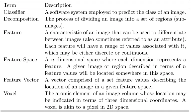
Table 2.1: Terminology used throughout this thesis

Term Description

Classifier A software system employed to predict the class of an image. Decomposition The process of dividing an image into a set of regions

(sub-images).

Feature A characteristic of an image that can be used to differentiate between images (also sometimes referred to as an attribute). Each feature will have a range of values associated with it, which may be either discrete or continuous.

Feature Space A n dimensional space where each dimension represents a feature. A given image or region described in terms of n

feature values will be located somewhere in this space. Feature Vector A vector comprised of a set feature values describing the

location of an image in a given feature space.

Voxel The atomic element of an image volume whose location may be indicated in terms of three dimensional coordinates. A voxel is akin to a pixel in 2D space.

Table 2.2: Basic notation used throughout this thesis

Notation Description

In An imagenin the dataset I.

Cn The class label for imagen in the dataset I.

X×Y ×Z The size of an image, where X, Y and Z are the width, height, and depth of the image respectively.

In(x, y, z) A voxel within an image of a given x, y, z location, where

x∈X,y∈Y and z∈Z.

AIVi The average intensity value of a regioni.

d(i, j) A function to measure the difference or similarity between two given vectors or valuesi,j.

(29)

2.2 Knowledge Discovery in Images

As noted in the introduction to this chapter, the field of Knowledge Discovery in Im-ages (KDI) is a specialised variant of the more general field of Knowledge Discovery in Databases (KDD). The distinction between KDI and KDD is thus discussed in Subsec-tion 2.2.1. SubsecSubsec-tion 2.2.2 then presents a categorisaSubsec-tion of the applicaSubsec-tion-dependent objectives of KDI and this is followed in Subsection 2.2.3 by a general review of the KDI process.

2.2.1 Distinction Between KDI and KDD

The fundamental distinction between KDD and KDI is that the latter is intended to be applied specifically to image data, while KDD has much more general applicability. KDD is defined as the process of identifying useful knowledge from data, while data mining is the sub-process within the overall KDD process concerned with the actual identification of hidden information. The focus of KDI is to support the automated extraction of information from images (as opposed to data in general). KDI is thus concerned with methods for mapping low-level features in images to descriptions where the relationships between them are hidden [64]. KDD is concerned with knowledge discovery in (relational) databases, while KDI is concerned with knowledge discov-ery in image data. However, there are some significant differences between relational databases and image databases which in turn require that some sub-processes within the overall KDI process need to be different to the corresponding processes found in KDD. Thus this section reviews the distinctions between image data and tabular data so as to highlight the differences between the KDI and KDD processes. The differences between relational databases and image databases data may be summarised as follows [60, 154]:

1. Absolute versus relative values: Usually, in relational databases values are meaningful on their own, such as the value for an attribute age. In contrast, the intensity value of an image pixel/voxel does not reveal much information on its own unless the neighbouring context is considered. Therefore, individual intensity values need to be considered with respect to their neighbours.

(30)

of an image without considering this spatial information. In relational databases, there is no need to consider such spatial relationships.

3. Unique versus multiple interpretation: In tabular data, the data has a unique interpretation. In contrast, in the case of images it may be the case that the same region can have multiple interpretations. A robust feature extraction method which can cope with this issue therefore needs to be used.

From the above, the main distinction between KDI and KDD is that image data tends to be very unstructured while the tabular data to which KDD is normally ap-plied tends to be highly structured. Thus a variety of processes, from across different disciplines (such as image processing and computer vision [85]), are needed to realise KDI. Feature extraction is one of the most dominant problems in KDI [34]. This issue will therefore be discussed in further detail in Section 2.4.

2.2.2 Objectives of KDI

This subsection considers the distinctions between KDI and KDD further by consid-ering the objectives of KDI in comparison with KDD. At a high level the application-dependent objectives of both KDD and KDI can be characterised as being either: (i) descriptive knowledge discovery or (ii) predictive knowledge discovery [128]. In the case of KDI the focus of descriptive knowledge discovery is on how to describe or represent image data in as concise a manner as possible while at the same time ensuring that key elements of the data are not lost (so that previously hidden knowledge can be readily identified). In descriptive knowledge discovery the aim is to understand the content, differences and similarities of the given image data. For instance, an image may be represented in terms of features, such as texture or shape, so as to form a meaning-ful description. These descriptions can then be used to compare between images. In the KDD techniques applied to relational databases, descriptive knowledge discovery is not a significant issue because each value is meaningful in its own right, while in KDI descriptive knowledge discovery is a significant issue because individual values are not meaningful in their own right.

(31)

2.2.3 KDI Process

The KDI process comprises a sequence of steps similar to those found in KDD [75, 80]. The precise sequence and nature of these steps varies across KDI application domains and KDI methodologies. In the context of the work described in this thesis (which is directed at 3D image classification), the KDI process is considered to comprise the following sequence of steps:

1. Preprocessing Phase

(a) Dataset creation: This step is essentially concerned with image acquisi-tion.

(b) Preparation: Preparation of the 3D image data so as to remove unwanted structure, such as noise, so as to enhance the image quality.

(c) Image representation: The encapsulation of the key elements (features) of a given set of images (volumes)

(d) Feature vector generation: Generation of a set of feature vectors describ-ing the image data. Note that feature vector generation may also require the application of “reduction methods” so as to reduce the complexity/size of the feature space. This may only be needed if the quantity of generated feature vectors cannot be handled within the image mining.

2. Data Mining Phase

(a) Image mining: The step in which the actual knowledge discovery is un-dertaken (classifier generation with respect to the work described in this thesis).

3. Post Processing and Usage Phase

(a) Evaluation:: The evaluation of the discovered knowledge (the generated classifier).

(b) Usage: Application of the discovered knowledge (usage of the generated classifier to label previously unseen volumes)

Note that the above is divided into three phases: (i) preprocessing, (ii) mining and (iii) post-processing and usage. Each of these phases is discussed in further detail in the following three subsections.

2.2.3.1 The KDI Preprocessing Phase

(32)

of objects acquired by some process. The image acquisition process can be affected by factors such as: (i) noise, (ii) resolution and (iii) configuration settings. As a result, the nature of the acquired images is often changeable. Therefore, various preliminary processes need to be applied to the images such as colour equalisation, noise removal, and image alignment (registration) [154].

The next step is to represent an image in some way. Image representation in the specific context of the work described later in this thesis is discussed in Sections 2.4 and 2.5. Whatever the case, the nature of the chosen image representations is critical to the effectiveness of the nature of the KDI to be applied [5, 8]. The general aim is to represent image data in terms of a set of features. In the context of the work described in this thesis, the identified set of features should be compatible with the concept of a feature vector representation. The challenges are firstly how best to decide what features are most appropriate to the selected KDI task and secondly how best to extract the desired features. Typically, depending on the application domain, we wish to preserve one or more of the following: contextual information, spatial information, texture and connectivity.

There are a variety of ways that we might represent image data. A growing amount of research has focused on building “local” based image representations. The term “local” in the context of representation refers to the building of descriptors for parts (sub-images) of the whole image (i.e. a local grouping of pixels/voxels). Local based image representations are thus concerned with features that describe a small region within an image instead of a whole image. Local invariant features have proven effective for a range of computer vision problems over the last decade [151]. Local image based representation requires that the given image is first decomposed into a collection of sub-images/sub-volumes (called regions). Mechanisms for this are well understood. The main issue is how to select a representation for the identified regions that allows them to be used to discriminate between images. For classification purposes each image should be represented in a way that makes its label distinguishable from other class labels.

Once we have described our image set in terms of a set of appropriate features the next step is typically to generate a set of feature vectors. The objective of feature vector generation is to include only the most relevant features. Thus in this stage irrelevant or redundant features are removed [12]. In the case of image classification we also wish to retain features with a high discriminatory power.

2.2.3.2 The KDI Mining Phase

(33)

so that IM can be applied and the post-processing of the discovered knowledge so that it can be used with respect to some application domain context. The challenge of IM is how to effectively extract the desired knowledge [60]. IM, like data mining in general, makes use of techniques taken from a number of different domains including: machine learning, statistics and artificial intelligence [11, 102].

In the context of image classification the goal of the IM is classifier generation. The input to the classifier generator is a set of training images I = {I1, ...., In}, with the associated training labelsC ={c1, ....cn}. The output is a mapping of the input to the set of class labels: f :χ→C.

2.2.3.3 The KDI Post Processing and Usage Phase

On completion of the IM phase the acquired knowledge can be applied. In the case of image classification this means the application of the generated classifier to real-life data. Prior to this it is useful to obtain some level of confidence in the generated classifier. This is typically done by applying the classifier to pre-labelled test data. There are a number of different evaluation metrics that can be used to measure the performance of a classifier. Further details concerning these metrics are presented in Section 2.8.

2.3 Hierarchical Spatial Decomposition

The work described in this thesis is directed at image representations for classification founded on the idea of hierarchical decomposition. Image decomposition has been used in various application domains [118]: such as computer graphics [63, 65], volume ren-dering [42, 120], modelling and animation [17], segmentation [87, 141] and Geographic Information Systems [10]. In [133] an edge detection algorithm was proposed using image decomposition.

The basic idea is to decompose a given image In into a set of sub-images (called regions in this thesis). Image decomposition offers a number of advantages that can be summarised as follows (see also [13, 137, 144]):

1. General applicability.

2. Provides for a more effective representation (than other methods) because it al-lows for the capture of regionalised details.

3. Fast computation of image properties due to applying representation methods to small regions.

(34)

5. Provides for a simplification of the space.

6. In many cases obviates the need for computationally expensive processes such as segmentation.

7. Reduces problems associated with occlusion because of the use of smaller regions instead of the whole image

The process of decomposition has to satisfy a number of conditions in order to ensure that appropriate regions are identified. These are itemised in [137] as follows:

1. Repeatable: The same regions should be identified in different conditions.

2. Robust: The decomposition should be robust against factors such as occlusion, clutter, noise and blur.

3. Homogeneity: The identified regions should, in some sense, be homogeneous.

4. Invariant: The decomposition should be invariant against transformations and deformations.

5. Distinctive: Allow for individual regions to be matched to similar regions in other images.

6. Quantity: Result in a sufficient number of regions with respect to the envisioned application.

7. Efficient: Operate in an efficient manner.

There are various different spatial decomposition methods that can be found in the literature. Subsection 2.3.1 below provides an overview of some of the most popular methods. One of the issues with hierarchical decomposition is deciding when to stop. One approach is to define a maximum “level” for the decomposition. However, on its own, this might result in unnecessary decomposition. A more efficient approach is to cease decomposing a branch whenever a homogeneous region is arrived at. There are various mechanisms for measuring regional homogeneity, usually expressed in terms of what is referred to as acritical function, and these are reviewed in Subsection 2.3.2.

2.3.1 Spatial Decomposition Methods

(35)

which, as the name suggests, requires recourse to segmentation algorithms. Popular segmentation techniques used for this purpose are Watershed [23] and Superpixel [114]. The disadvantages of segmentation-based approaches are:

1. Good-quality images are required. Image blurring can make it difficult to iden-tify image boundaries and consequently the segmentation process is less accurate [95]. One potential solution is to use the concept of “region isophotes” to handle problems associated within boundary blurring [103].

2. Many very small objects may be identified. One idea whereby this issue may be addressed is to use some threshold, such as the “Maximally Stable” condition used in [94], but this in turn means that the segmentation does not necessarily cover the whole image.

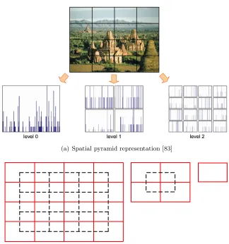
The advantage of the segmentation-based approaches is that the “overlap” prob-lem found in grid-based representations does not occur. This is where an object of interest is distributed over a number of different regions dispersed across the decom-position, which in some cases can hinder further analysis. It is the view of the author that the disadvantages associated with segmentation-based decomposition outweighed the advantages, and thus the work described in this thesis is directed at grid-based decomposition techniques.

(36)

(a) Spatial pyramid representation [83]

[image:36.612.155.479.72.418.2]

(b) Overlapped MSSP representation where the red lines indicate the overlapped regions [146]

Figure 2.1: Forms of grid decomposition.

2.3.2 Regional Homogeneity

As noted above, homogeneity is an important issue in the context of image decompo-sition. With respect to image decomposition, homogeneity is measured using what is referred to as a “critical function”. Most existing critical functions are typically in-tended for use with segmentation-based methods [135]. These methods are applied to extract homogeneous regions (segments). In order to determine the homogeneity of a region, statistical features of the region or edges are taken into consideration [41]. In the literature, there are two common examples of critical functions based on statistical features: (i) Average Intensity Values (AIV) (mean) [59] and (ii) Kendall’s Coefficient Concordance (KCC) [153]. With respect to edge information proposed methods are prone to failure when the adapted edge detection mechanism fails to identify all edges, leading to over/under-segmentation [41].

(37)

con-text of 2D image decomposition. The AIV value of each region is computed before decomposition. Then the region is decomposed and the AIV for each child sub-region is computed. Following this, a difference function is constructed to compute the “dis-tance” d(AIVp, AIVi) = AIVp−AIVi between the parent region AIVp and the AIV of each child region AIVi. The square root of the sum of the distances between the parent region and the child regions is then computed. The homogeneityωof the parent volume is calculated using Equation 2.1, wheres is the number of child regions,AIVp indicates the parent AIV and AIVi the AIV for each child region. If the value of ω is less than a predefined threshold the region is considered to be homogeneous and therefore the decomposition process is stopped. A similar approach using the mean intensity value was used with respect to the region growing method described in [30]. AIV was included as a feature in the MPEG-7 algorithm [147].

ω= 1

s

s X

i=1

q

(AIVp−AIVi)2 (2.1)

KCC was proposed in [153] where it was used to assess the homogeneity of regions in functional MRI (fMRI) images. KCC is a time-series based method for measuring the relationships between each voxel and its neighbours. In the context of 3D volumes KCC operates as follows. First, for each voxel in a decomposed region, a time series involving the intensity values of the voxel’s nearest neighbours is formed. Then the KCC is applied on the generated time series to check the homogeneity of the region. KCC is calculated using Equation 2.2.

KCC=

P

(R2_i −nR¯2)

1/12K2₍_n3₋_n₎ (2.2)

whereRi is the sum of theith time series for theith voxel, ¯R= (n+1)₂ K, ¯Ris the mean of each time series, K is the size of the time series (number of selected neighbours for each voxel) andnis the number of voxels in a given region. The resultingKCC value has a range of 0 to 1, where 1 indicates a completely homogeneous region and 0 an entirely un-homogeneous region.

Note that AIV and KCC are both used later in this thesis for comparison with the author’s own proposed critical functions.

2.4 Region-based Representation

(38)

equally well be applied in the context of whole, non-decomposed, image representa-tion). From the literature, two categories of region-based representation can be identi-fied: (i) statistical-based techniques and (ii) histogram-based techniques. Two types of statistical-based techniques can also be identified: (i) first-order and (ii) second-order [134]. In the case of first-order methods, images are described using statistical functions such as mean, variance, energy and standard deviation of the image’s intensity values. With respect to the second-order methods, the relationship between the intensity value of each pixel with respect to those of its neighbours is taken into considera-tion [134]. In other words, relative locaconsidera-tion informaconsidera-tion is used. One example of a second-order method is where the concept of a co-occurrence matrix [44, 49] is used to enumerate the number of times two intensity values appear in an image within a certain distance and a direction of each other. A Voxel Co-occurrence Matrix (VCM) is used in the same manner as a pixel co-occurrence matrix but with respect to 3D images [44]. In a VCM matrix, the rows and the columns represent intensity values and a field represents the frequency that an intensity value in theith row was adjacent to the intensity value in the jth column. The adjacency is defined by a displacement distance d and angle. After computing VCM, various statistical functions can be ap-plied to this matrix, such as angular second moment, contrast, correlation and variance. Another example of a second-order method is where run-length encoding matrices are used. These are matrices that hold information about the set of consecutive intensity pixels/voxels that have the same values [43, 132]. A Voxel Run-Length Matrix (VRLM) is the 3D form of a pixel run-length matrix. In a VRLM matrix, the rows represent intensity values, the columns represent the length of the run and the fields show the frequency of a specific intensity value in adjacent pixels/voxels in a specific direction. Similar to VCM, in the case of the VRLM matrix, different functions may be applied, such as, short/long run emphasis, length nonuniformity, run percentage and so on.

Regardless of whether first-order or second-order statistical methods are used, the generated statistics describe individual features which in turn can be used to define a feature space from which feature vectors can be extracted.

(39)

only the frequency of the intensity values are considered; and (ii) invariant problems, especially when two images have similar content but with different resolutions (in which case different histograms will be produced).

A more advanced histogram-based method is the use of Histograms of Oriented Gradients (or HOGs) [24]. Using HOGs the changes in the intensity values of the region, with respect to either the azimuth and/or zenith direction, are computed and referred to asgradients. In order to compute a gradient at each location the difference between the “left” and “right” neighbouring intensity values, in a given direction, is calculated. Following this, the angles between the image gradients are computed and stored in what are called “orientation” bins. The gradient magnitudes in each orientation bin are accumulated. In the generated histogram, the x-axis represents directions and the y-axis the sum of the gradient magnitudes.

In order to generate LBPs, each pixel/voxel is compared to its immediate neigh-bours. For each comparison a one is stored if the intensity value of the pixel/voxel is greater than the neighbour, otherwise a zero is stored. The generated binary number from the sequence of neighbours then describes an integer value. In the generated his-togram, the x-axis represents the computed integer values and the y-axis the frequency with which they occur. In order to generate a robust representation, it is desirable to compute rotation invariant LBPs. With respect to 2D images it is straightforward to calculate rotation invariant LBPs because each location has only eight immediate neighbours. With respect to 3D images the generation of 3D rotation invariant LBPs (26 neighbours in contrast to 8 neighbours) is computationally expensive. To address this issue Zhao and Pietikainen [157] proposed the use of Three Orthogonal Plane LBPs (LBP-TOP). The LBP-TOP representation considers the calculation of LBPs only with respect to neighbouring voxels located in the XY, XZ and Y Z planes. A combina-tion of HOG and LBP (HOG-LBP) has also been proposed and found to be a robust representation [143].

The concept of histograms of Local Phase Quantisation (LPQ) was proposed in [101]. LPQ uses low frequency local Fourier transforms whereby a histogram of the quantised Fourier transform can be generated [99]. At each image location, a Short-Term Fourier Transform (STFT) is applied with respect to the immediate neighbours. Then the resulting values are quantised (a value of one is used if the value is bigger than or equal to zero, otherwise a value of zero is used). In this manner a binary encoding is computed for each image location which can then be interpreted as an integer value between 0-256 (b = P8

i=0qi2i

−1_{, where} _q

(40)

2.5 Whole Image-Based Representation

An alternative to representing individual regions is to represent the decomposition in its entirety, for example as some form of tree which can eventually be translated into a feature vector format (again to ensure compatibility with the data mining techniques to later be applied). There are a variety of mechanisms whereby this can be achieved that have been reported in the literature; however, hierarchical decomposition techniques naturally lend themselves to tree representations where the nodes represent regions. The question is then what features to store at the tree nodes (and by extension the links connecting the nodes); in other words, what information should the tree hold?

There has been a substantial amount of work directed at tree based representations of space but mostly directed at 2D space such as [31] and [59]. In [31] a quad tree representation was used to encapsulate a 2D representation of the Corpus Callosum, the part of the brain that connects the left and right hand sides of the brain. The shape of the Corpus Callosum was extracted from MRI scan data. In this case, the data stored at the tree nodes was either the digit 1 or the digit 0, 1 indicating that the associated region was part of the Corpus Callosum and 0 indicating it was not. The work of [59] is particularly relevant with respect to the work described in this thesis because a hierarchical representation was used to describe 2D retinal images. In this case, each node held the mean intensity values of all the pixels in the associated region [59].

What is interesting about tree representations is that a tree is a type of graph and therefore graph mining techniques can be applied. For example, frequently occurring sub-graphs (sub-trees) can be used as attributes in a feature space model. Both [31] and [59] experimented with this idea. A similar idea is adapted with respect to the work described in this thesis and hence graph mining is considered in some further detail below in Subsection 2.6.2.

2.6 Feature Vector Generation

(41)

are therefore discussed in Subsection 2.6.2.

2.6.1 Feature Vector Generation for Region-based Methods

Two commonly used methods used to reduce the dimensionality of a given feature space are: (i) Principal Component Analysis (PCA) and (ii) the coding-pooling framework. In PCA [69] orthogonal linear transforms are applied to the set of feature vectors, forming a new set of vectors according to the variance of the feature vectors. PCA is used to transform a feature space into lower-dimensional space. PCA operates by first calculating the Eigenvectors and Eigenvalues for the new space. Feature vectors are then generated using the list of Eigenvectors. They are sorted and a specific number of Eigenvectors are chosen. There is an assumption that an Eigenvector with a larger Eigenvalue indicates that this Eigenvector is significant, so Eigenvectors with the largest Eigenvalues are selected to represent the image [146].

In the coding-pooling framework the coding element consists of identifying a subset of vectors (the “dictionary”). The pooling element is then used to generate a single feature vector guided by the dictionary where feature vectors linked to the same vec-tor in the dictionary are combined. The coding should operate so that the selected vectors include the most representative features. There are different ways of conduct-ing the codconduct-ing, of note are: (i) Vector Quantization (VQ), (ii) Sparse Codconduct-ing (SC), (iii) Locality-constrained Linear Coding (LLC), (iv) Improved Fisher Kernel Encoding (IFK) and (v) SuperVector encoding (SV).

(42)

class-specific information. Similar to IFK, SuperVector (SV) encoding was used in [158]. Instead of GMM as in IFK, K-means clustering was computed. Then the clusters were improved by using upper bounds aimed at minimising the error using the Euclidean distance between feature vectors and their means. In [62] an experiment is reported that compares the operation of different coding methods; FK proposed in [105] was shown to outperform the rest.

With respect to the pooling element of the coding-pooling framework, the aim is to map each feature vector with its equivalent vector in the dictionary in order to form a single feature vector. There are two common methods for achieving this, average and maximum pooling. In “average pooling”, the average values between similar feature vector elements in the dictionary are computed and then used to form a new feature vector. Following this, a long global feature vector is generated by concatenating the new feature vectors for each image. The resulting feature vector is then normalised [82]. One example of maximum pooling is Multi-scale Spatial Maximum Pooling (MSMP) [149]. MSMP recursively computes the histograms of the maximum values for a given set of vectors and their association with elements in the dictionary. Feature vectors in neighbouring regions are recursively united by getting the maximum values of each element. This process of combing feature vectors is applied until a final single feature vector is reached.

2.6.2 Feature Vector Generation for Whole Image-based Methods As noted above, the generation of feature vectors from tree-based representations is more challenging than in the case of region-based representation methods. One ap-proach, used in [59] in the context of 2D retinal images and in [89] with respect to MRI brain scan data, is to first identify frequently occurring sub-graphs in the tree data using some appropriate search method. Various Frequent Sub-Graph (FSG) mining techniques can be used for this purpose. One of the most commonly used is the graph-based Substructure pattern mining (gSpan) algorithm [148]. The gSpan algorithm uses a Depth First Search (DFS) approach to identify frequent sub-graphs (sub-trees). A sub-graph is said to be frequent according to a “support threshold” σ. In the case of the tree representations considered in this thesis, each identified frequent sub-tree is then conceptualised as a dimension within a feature space. Sub-graphs may be ranked according to some weighting measure as suggested in [15] and the top K sub-graphs selected. This later approach was adapted in [59] in the context of 2D retinal images.