Chapter 8
kNN: k-Nearest Neighbors
Michael Steinbach and Pang-Ning Tan
Contents
8.1 Introduction . . . .151
8.2 Description of the Algorithm . . . .152
8.2.1 High-Level Description . . . .152
8.2.2 Issues . . . .153
8.2.3 Software Implementations . . . .155
8.3 Examples . . . .155
8.4 Advanced Topics. . . .157
8.5 Exercises . . . .158
Acknowledgments. . . .159
References . . . .159
8.1
Introduction
One of the simplest and rather trivial classifiers is the Rote classifier, which memorizes the entire training data and performs classification only if the attributes of the test object exactly match the attributes of one of the training objects. An obvious problem with this approach is that many test records will not be classified because they do not exactly match any of the training records. Another issue arises when two or more training records have the same attributes but different class labels.
A more sophisticated approach, k-nearest neighbor (kNN) classification [10,11,21], finds a group of k objects in the training set that are closest to the test object, and bases the assignment of a label on the predominance of a particular class in this neighborhood. This addresses the issue that, in many data sets, it is unlikely that one object will exactly match another, as well as the fact that conflicting information about the class of an object may be provided by the objects closest to it. There are several key elements of this approach: (i) the set of labeled objects to be used for evaluating a test object’s class,1(ii) a distance or similarity metric that can be used to compute
the closeness of objects, (iii) the value of k, the number of nearest neighbors, and (iv) the method used to determine the class of the target object based on the classes and distances of the k nearest neighbors. In its simplest form, kNN can involve assigning an object the class of its nearest neighbor or of the majority of its nearest neighbors, but a variety of enhancements are possible and are discussed below.
More generally, kNN is a special case of instance-based learning [1]. This includes case-based reasoning [3], which deals with symbolic data. The kNN approach is also an example of a lazy learning technique, that is, a technique that waits until the query arrives to generalize beyond the training data.
Although kNN classification is a classification technique that is easy to understand and implement, it performs well in many situations. In particular, a well-known result by Cover and Hart [6] shows that the classification error2of the nearest neighbor rule
is bounded above by twice the optimal Bayes error3under certain reasonable
assump-tions. Furthermore, the error of the general kNN method asymptotically approaches that of the Bayes error and can be used to approximate it.
Also, because of its simplicity, kNN is easy to modify for more complicated classifi-cation problems. For instance, kNN is particularly well-suited for multimodal classes4
as well as applications in which an object can have many class labels. To illustrate the last point, for the assignment of functions to genes based on microarray expression profiles, some researchers found that kNN outperformed a support vector machine (SVM) approach, which is a much more sophisticated classification scheme [17].
The remainder of this chapter describes the basic kNN algorithm, including vari-ous issues that affect both classification and computational performance. Pointers are given to implementations of kNN, and examples of using the Weka machine learn-ing package to perform nearest neighbor classification are also provided. Advanced techniques are discussed briefly and this chapter concludes with a few exercises.
8.2
Description of the Algorithm
8.2.1
High-Level Description
Algorithm 8.1 provides a high-level summary of the nearest-neighbor classification method. Given a training set D and a test object z, which is a vector of attribute values and has an unknown class label, the algorithm computes the distance (or similarity)
2The classification error of a classifier is the percentage of instances it incorrectly classifies.
3The Bayes error is the classification error of a Bayes classifier, that is, a classifier that knows the underlying
probability distribution of the data with respect to class, and assigns each data point to the class with the highest probability density for that point. For more detail, see [9].
4With multimodal classes, objects of a particular class label are concentrated in several distinct areas of
8.2 Description of the Algorithm 153
Algorithm 8.1 Basic kNN Algorithm
Input : D, the set of training objects, the test object, z, which is a vector of attribute values, and L, the set of classes used to label the objects Output : cz ∈L, the class of z
foreach object y∈ D do
|Compute d(z,y), the distance between z and y; end
Select N ⊆D, the set (neighborhood) of k closest training objects for z; cz=argmax
v∈L
y∈N I (v=class(cy));
where I (·) is an indicator function that returns the value 1 if its argument is true and 0 otherwise.
between z and all the training objects to determine its nearest-neighbor list. It then assigns a class to z by taking the class of the majority of neighboring objects. Ties are broken in an unspecified manner, for example, randomly or by taking the most frequent class in the training set.
The storage complexity of the algorithm is O(n), where n is the number of training objects. The time complexity is also O(n), since the distance needs to be computed between the target and each training object. However, there is no time taken for the construction of the classification model, for example, a decision tree or sepa-rating hyperplane. Thus, kNN is different from most other classification techniques which have moderately to quite expensive model-building stages, but very inexpensive O(constant) classification steps.
8.2.2
Issues
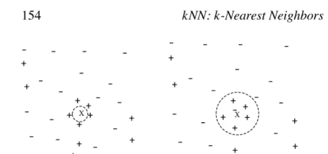
There are several key issues that affect the performance of kNN. One is the choice of k. This is illustrated in Figure 8.1, which shows an unlabeled test object, x, and training objects that belong to either a “+” or “−” class. If k is too small, then the result can be sensitive to noise points. On the other hand, if k is too large, then the neighborhood may include too many points from other classes. An estimate of the best value for k can be obtained by cross-validation. However, it is important to point out that k=1 may be able to perform other values of k, particularly for small data sets, including those typically used in research or for class exercises. However, given enough samples, larger values of k are more resistant to noise.
Another issue is the approach to combining the class labels. The simplest method is to take a majority vote, but this can be a problem if the nearest neighbors vary widely in their distance and the closer neighbors more reliably indicate the class of the object. A more sophisticated approach, which is usually much less sensitive to the choice of k, weights each object’s vote by its distance. Various choices are possible; for example, the weight factor is often taken to be the reciprocal of the squared distance:
+ +‒ ‒ ‒ ‒ ‒ ‒ ‒ ‒ ‒ ‒ ‒ ‒ ‒ ‒ ‒ ‒ ‒ ‒ ‒ ‒ + + + X + + + + + + ‒ ‒ ‒ ‒ ‒ ‒ ‒ ‒ ‒ ‒ ‒ ‒ ‒ ‒ ‒ ‒ ‒ ‒ ‒ ‒ ‒ + + + + + + + + + + + X ‒ ‒ ‒ ‒ ‒ ‒ ‒ ‒ ‒ ‒ ‒ ‒ ‒ ‒ ‒ ‒ ‒ ‒ ‒ ‒ ‒ + + + + + + + + + + + X
(a) Neighborhood too small.
(b) Neighborhood just right.
[image:4.612.57.394.49.208.2](c) Neighborhood too large.
Figure 8.1 k-nearest neighbor classification with small, medium, and large k.
following:
Distance-Weighted Voting: cz =argmax
v∈L
y∈N
wi×I (v=class(cy)) (8.1)
The choice of the distance measure is another important consideration. Commonly, Euclidean or Manhattan distance measures are used [21]. For two points, x and y, with n attributes, these distances are given by the following formulas:
d(x,y) =
n
k=1
(xk−yk)2 Euclidean distance (8.2)
d(x,y) =
n
k=1
|xk−yk| Manhattan distance (8.3)
where xkand ykare the kt hattributes (components) of x and y, respectively.
Although these and various other measures can be used to compute the distance between two points, conceptually, the most desirable distance measure is one for which a smaller distance between two objects implies a greater likelihood of having the same class. Thus, for example, if kNN is being applied to classify documents, then it may be better to use the cosine measure rather than Euclidean distance. Note that kNN can also be used for data with categorical or mixed categorical and numerical attributes as long as a suitable distance measure can be defined [21].
8.3 Examples 155
the weight of a person varies from 90 to 300 lb, and the income of a person varies from $10,000 to $1,000,000. If a distance measure is used without scaling, the income attribute will dominate the computation of distance, and thus the assignment of class labels.
8.2.3
Software Implementations
Algorithm 8.1 is easy to implement in almost any programming language. However, this section contains a short guide to some readily available implementations of this algorithm and its variants for those who would rather use an existing implementation. One of the most readily available kNN implementations can be found in Weka [26]. The main function of interest is IBk, which is basically Algorithm 8.1. However, IBk also allows you to specify a couple of choices of distance weighting and the option to determine a value of k by using cross-validation.
Another popular nearest neighbor implementation is PEBLS (Parallel Exemplar-Based Learning System) [5,19] from the CMU Artificial Intelligence repository [20]. According to the site, “PEBLS (Parallel Exemplar-Based Learning System) is a nearest-neighbor learning system designed for applications where the instances have symbolic feature values.”
8.3
Examples
In this section we provide a couple of examples of the use of kNN. For these examples, we will use the Weka package described in the previous section. Specifically, we used Weka 3.5.6.
To begin, we applied kNN to the Iris data set that is available from the UCI Machine Learning Repository [2] and is also available as a sample data file with Weka. This data set consists of 150 flowers split equally among three Iris species: Setosa, Versicolor, and Virginica. Each flower is characterized by four measurements: petal length, petal width, sepal length, and sepal width.
The Iris data set was classified using the IB1 algorithm, which corresponds to the IBk algorithm with k=1. In other words, the algorithm looks at the closest neighbor, as computed using Euclidean distance from Equation 8.2. The results are quite good, as the reader can see by examining the confusion matrix5given in Table 8.1.
However, further investigation shows that this is a quite easy data set to classify since the different species are relatively well separated in the data space. To illustrate, we show a plot of the data with respect to petal length and petal width in Figure 8.2. There is some mixing between the Versicolor and Virginica species with respect to
5A confusion matrix tabulates how the actual classes of various data instances (rows) compare to their
TABLE 8.1
Confusion Matrix for Weka kNN Classifier IB1 on the Iris Data SetActual/Predicted Setosa Versicolor Virginica
Setosa 50 0 0
Versicolor 0 47 3
Virginica 0 4 46
their petal lengths and widths, but otherwise the species are well separated. Since the other two variables, sepal width and sepal length, add little if any discriminating information, the performance seen with basic kNN approach is about the best that can be achieved with a kNN approach or, indeed, any other approach.
The second example uses the ionosphere data set from UCI. The data objects in this data set are radar signals sent into the ionosphere and the class value indicates whether or not the signal returned information on the structure of the ionosphere. There are 34 attributes that describe the signal and 1 class attribute. The IB1 algorithm applied on the original data set gives an accuracy of 86.3% evaluated via tenfold cross-validation, while the same algorithm applied to the first nine attributes gives an accuracy of 89.4%. In other words, using fewer attributes gives better results. The confusion matrices are given below. Using cross-validation to select the number of nearest neighbors gives an accuracy of 90.8% with two nearest neighbors. The confusion matrices for these cases are given below in Tables 8.2, 8.3, and 8.4, respectively. Adding weighting for nearest neighbors actually results in a modest drop in accuracy. The biggest improvement is due to reducing the number of attributes.
Petal width
Petal length 2.5
1
1.5
1
0.5
0
Setosa Versicolor Virginica
1 2 3 4 5 6 7
8.4 Advanced Topics 157
TABLE 8.2
Confusion Matrix for Weka kNN Classifier IB1 on the Ionosphere Data Set Using All AttributesActual/Predicted Good Signal Bad Signal
Good Signal 85 41
Bad Signal 7 218
8.4
Advanced Topics
To address issues related to the distance function, a number of schemes have been developed that try to compute the weights of each individual attribute or in some other way determine a more effective distance metric based upon a training set [13, 15]. In addition, weights can be assigned to the training objects themselves. This can give more weight to highly reliable training objects, while reducing the impact of unreliable objects. The PEBLS system by Cost and Salzberg [5] is a well-known example of such an approach.
As mentioned, kNN classifiers are lazy learners, that is, models are not built explic-itly unlike eager learners (e.g., decision trees, SVM, etc.). Thus, building the model is cheap, but classifying unknown objects is relatively expensive since it requires the computation of the k-nearest neighbors of the object to be labeled. This, in general, requires computing the distance of the unlabeled object to all the objects in the la-beled set, which can be expensive particularly for large training sets. A number of techniques, e.g., multidimensional access methods [12] or fast approximate similar-ity search [16], have been developed for efficient computation of k-nearest neighbor distance that make use of the structure in the data to avoid having to compute distance to all objects in the training set. These techniques, which are particularly applicable for low dimensional data, can help reduce the computational cost without affecting classification accuracy. The Weka package provides a choice of some of the multi-dimensional access methods in its IBk routine. (See Exercise 4.)
Although the basic kNN algorithm and some of its variations, such as weighted kNN and assigning weights to objects, are relatively well known, some of the more advanced techniques for kNN are much less known. For example, it is typically possible to eliminate many of the stored data objects, but still retain the classification accuracy of the kNN classifier. This is known as “condensing” and can greatly speed up the classification of new objects [14]. In addition, data objects can be removed to
TABLE 8.3
Confusion Matrix for Weka kNN Classifier IB1 on the Ionosphere Data Set Using the First Nine AttributesActual/Predicted Good Signal Bad Signal
Good Signal 100 26
[image:7.612.103.349.559.601.2]TABLE 8.4
Confusion Matrix for Weka kNN Classifier IBk on the Ionosphere Data Set Using the First Nine Attributes with k =2Actual/Predicted Good Signal Bad Signal
Good Signal 103 9
Bad Signal 23 216
improve classification accuracy, a process known as “editing” [25]. There has also been a considerable amount of work on the application of proximity graphs (nearest neighbor graphs, minimum spanning trees, relative neighborhood graphs, Delaunay triangulations, and Gabriel graphs) to the kNN problem. Recent papers by Toussaint [22–24], which emphasize a proximity graph viewpoint, provide an overview of work addressing these three areas and indicate some remaining open problems.
Other important resources include the collection of papers by Dasarathy [7] and the book by Devroye, Gyorfi, and Lugosi [8]. Also, a fuzzy approach to kNN can be found in the work of Bezdek [4]. Finally, an extensive bibliography on this subject is also available online as part of the Annotated Computer Vision Bibliography [18].
8.5
Exercises
1. Download the Weka machine learning package from the Weka project home-page and the Iris and ionosphere data sets from the UCI Machine Learning Repository. Repeat the analyses performed in this chapter.
2. Prove that the error of the nearest neighbor rule is bounded above by twice the Bayes error under certain reasonable assumptions.
3. Prove that the error of the general kNN method asymptotically approaches that of the Bayes error and can be used to approximate it.
4. Various spatial or multidimensional access methods can be used to speed up the nearest neighbor computation. For the k-d tree, which is one such method, estimate how much the saving would be. Comment: The IBk Weka classification algorithm allows you to specify the method of finding nearest neighbors. Try this on one of the larger UCI data sets, for example, predicting sex on the abalone data set.
5. Consider the one-dimensional data set shown in Table 8.5.
TABLE 8.5
Data Set for Exercise 5x 1.5 2.5 3.5 4.5 5.0 5.5 5.75 6.5 7.5 10.5
References 159
(a) Given the data points listed in Table 8.5, compute the class of x = 5.5 according to its 1-, 3-, 6-, and 9-nearest neighbors (using majority vote). (b) Repeat the previous exercise, but use the weighted version of kNN given
in Equation (8.1).
6. Comment on the use of kNN when documents are compared with the cosine measure, which is a measure of similarity, not distance.
7. Discuss kernel density estimation and its relationship to kNN.
8. Given an end user who desires not only a classification of unknown cases, but also an understanding of why cases were classified the way they were, which classification method would you prefer: decision tree or kNN?
9. Sampling can be used to reduce the number of data points in many kinds of data analysis. Comment on the use of sampling for kNN.
10. Discuss how kNN could be used to perform classification when each class can have multiple labels and/or classes are organized in a hierarchy.
Acknowledgments
This work was supported by NSF Grant CNS-0551551, NSF ITR Grant ACI-0325949, NSF Grant IIS-0308264, and NSF Grant IIS-0713227. Access to computing facil-ities was provided by the University of Minnesota Digital Technology Center and Supercomputing Institute.
References
[1] D. W. Aha, D. Kibler, and M. K. Albert. Instance-based learning algorithms. Mach. Learn., 6(1):37–66, January 1991.
[2] A. Asuncion and D. Newman. UCI Machine Learning Repository, 2007.
[3] B. Bartsch-Sp¨orl, M. Lenz, and A. H¨ubner. Case-based reasoning—survey and future directions. In F. Puppe, editor, XPS-99: Knowledge-Based Systems—Survey and Future Directions, 5th Biannual German Conference on Knowledge-Based Systems, volume 1570 of Lecture Notes in Computer Sci-ence, W¨urzburg, Germany, March 3-5 1999. Springer.
[4] J. C. Bezdek, S. K. Chuah, and D. Leep. Generalized k-nearest neighbor rules. Fuzzy Sets Syst., 18(3):237–256, 1986.
[6] T. Cover and P. Hart. Nearest neighbor pattern classification. IEEE Transactions on Information Theory, 13(1):21–27, January 1967.
[7] B. Dasarathy. Nearest Neighbor (NN) Norms: NN Pattern Classification Tech-niques. Computer Society Press, 1991.
[8] L. Devroye, L. Gyorfi, and G. Lugosi. A Probabilistic Theory of Pattern Recog-nition. Springer-Verlag, 1996.
[9] R. O. Duda, P. E. Hart, and D. G. Stork. Pattern Classification (2nd Edition). Wiley-Interscience, November 2000.
[10] E. Fix and J. J. Hodges. Discriminatory analysis: Non-parametric discrimi-nation: Consistency properties. Technical report, USAF School of Aviation Medicine, 1951.
[11] E. Fix and J. J. Hodges. Discriminatory analysis: Non-parametric discrimina-tion: Small sample performance. Technical report, USAF School of Aviation Medicine, 1952.
[12] V. Gaede and O. G¨unther. Multidimensional access methods. ACM Comput. Surv., 30(2):170–231, 1998.
[13] E.-H. Han, G. Karypis, and V. Kumar. Text categorization using weight adjusted k-nearest neighbor classification. In PAKDD ’01: Proceedings of the 5th Pacific-Asia Conference on Knowledge Discovery and Data Mining, pages 53–65, London, UK, 2001. Springer-Verlag.
[14] P. Hart. The condensed nearest neighbor rule. IEEE Trans. Inform., 14(5):515– 516, May 1968.
[15] T. Hastie and R. Tibshirani. Discriminant adaptive nearest neighbor classifica-tion. IEEE Trans. Pattern Anal. Mach. Intell., 18(6):607–616, 1996.
[16] M. E. Houle and J. Sakuma. Fast approximate similarity search in extremely high-dimensional data sets. In ICDE ’05: Proceedings of the 21st Interna-tional Conference on Data Engineering, pages 619–630, Washington, DC, 2005. IEEE Computer Society.
[17] M. Kuramochi and G. Karypis. Gene classification using expression profiles: A feasibility study. In BIBE ’01: Proceedings of the 2nd IEEE International Symposium on Bioinformatics and Bioengineering, page 191, Washington, DC, 2001. IEEE Computer Society.
[18] K. Price. Nearest neighbor classification bibliography. http://www.visionbib. com/bibliography/pattern621.html, 2008. Part of the Annotated Computer Vision Bibliography.
References 161
[20] S. Salzberg. PEBLS: Parallel exemplar-based learning system. http://www. cs.cmu.edu/afs/cs/project/ai-repository/ai/areas/learning/systems/pebls/0.html, 1994.
[21] P.-N. Tan, M. Steinbach, and V. Kumar. Introduction to Data Minining. Pearson Addison-Wesley, 2006.
[22] G. T. Toussaint. Proximity graphs for nearest neighbor decision rules: Recent progress. In Interface-2002, 34th Symposium on Computing and Statistics, Montreal, Canada, April 17–20, 2002.
[23] G. T. Toussaint. Open problems in geometric methods for instance-based learn-ing. In Discrete and Computational Geometry, volume 2866 of Lecture Notes in Computer Science, pages 273–283, December 6–9, 2003.
[24] G. T. Toussaint. Geometric proximity graphs for improving nearest neighbor methods in instance-based learning and data mining. Int. J. Comput. Geometry Appl., 15(2):101–150, 2005.
[25] D. Wilson. Asymptotic properties of nearest neighbor rules using edited data. IEEE Trans. Syst., Man, and Cybernetics, 2:408–421, 1972.