Elliptic Combinatorics and Markov Processes

(1)

Elliptic Combinatorics and Markov Processes

Thesis by

Dan Betea

In Partial Fulfillment of the Requirements for the Degree of

Doctor of Philosophy

California Institute of Technology Pasadena, California

2012

(2)

c

2012

(3)

(4)

(5)

Acknowledgements

I would like to thank my adviser Eric Rains for his support during my graduate career. His knowledge on the subject of special functions in particular and on various related areas in general (combina-torics, representation theory, algebraic geometry of elliptic curves, etc.) is encyclopedic, and the benefits can be seen on most pages of this document. In addition to helping correct many mistaken computations, he has provided guidance and intuition on the project as a whole and made pertinent comments aimed at improving, strengthening, or streamlining results and/or proofs.

I would also like to thank Alexei Borodin for many helpful conversations, for guiding me at the beginning of the project, and for suggesting the project in the first place. Many results provided in this thesis (and more not yet in print) are generalizations of results he has been involved with one way or another.

In preparation for this manuscript I have also benefited from conversations with Tom Alberts, Fokko van de Bult, Sunil Chhita, Anton Geraschenko, Vadim Gorin, Rick Kenyon, and Ben Young. They have answered numerous questions I had on various issues, and for that I am extremely grateful. I would like to thank the Caltech math department staff and professors for making the graduate student experience here among the best anyone can hope for anywhere.

While a graduate student at Caltech, I have enjoyed the company of many wonderful friends. For all their support I will be eternally grateful. I am particularly indebted to Alexandra, Mihai, and Timea who in numerous private conversations have been forced to listen to my “complaints” about life and work in graduate school/academia.

(6)

(7)

Abstract

(8)

(9)

Introduction

In this chapter we start by addressing the purpose and layout of the thesis. We give a description of each subsequent chapter. We continue by introducing most of the notation and auxiliary functions necessary throughout, and finish with a brief overview of the uniformization theorem for elliptic curves.

1.1 Foreword

In this thesis we present certain combinatorial and probabilistic interpretations of recent results in the theory of elliptic special (hypergeometric) functions. On the special functions side we are interested in the multivariate results of Rains [Rai10], [Rai06] and on some univariate results due to Spiridonov and Zhedanov [SZ00] and Frenkel and Turaev [FT97]. On the statistical mechanical and probabilistic side we try to generalize results of Borodin, Gorin and Rains [BG09], [BGR10].

We mostly restrict attention to random elliptically distributed lozenge tilings of a hexagon. For such tilings, we first study many properties of the elliptic measures and explain how they are many parameter deformations of natural measures already studied on tilings. Tilings can be viewed as Markov processes and we provide theN-point correlation function as well as transition probabilities via Kasteleyn theory (equivalently, via the Lindstr¨om-Gessel-Viennot theorem). We interpret the transition probabilities as multivariate elliptic difference operators due to Rains. Properties of such operators also have nice probabilistic interpretations (i.e., quasi-commutation and quasi-adjointness) and allow us to couple two “orthogonal” Markov chains using ideas of Borodin and Ferrari [BF10] and to obtain an efficient polynomial-time sampling algorithm for random (large) elliptically distributed tilings. We provide computer simulations of the algorithm that lead to interesting asymptotic behavior of such tilings.

(12)

functions (generalizing skew Schur functions—see [Rai11]) and more precisely the elliptic binomial coefficients [Rai06]. Under certain specializations of the parameters such processes lead again to the elliptic measures we considered above. Identities for binomial coefficients and elliptic skew interpolation functions allow us to provide a second example of a polynomial-time efficient sampling algorithm (somewhat similar to the previous one, yet somewhat faster). We do this via a different coupling of two orthogonal Markov chains.

The layout of the thesis is as follows. For the rest of the first chapter we introduce the bulk of the notation used in all subsequent chapters. We also give some properties for some of the functions we introduce, restricting ourselves only to the necessary facts for our purposes. Finally we present a succinct description of the uniformization theorem that can oftentimes be useful when thinking about elliptic distributions. As a general note for the whole document, wherever our exposition follows one of the references closely, we make that point at the beginning of the respective section.

In Chapter2we collect a few recent results on elliptic hypergeometric functions. We are interested in univariate and multivariate evaluation formulas for integrals and summation formulas for termi-nating hypergeometric series. The most important results for our purposes are the Frenkel-Turaev summation formula and its multivariate analogue (see [FT97], [Rai06]) as well as a hypergeomet-ric determinant evaluation of Warnaar [War02]. We introduce the combinatorial and probabilistic aspects of lozenge tilings of a hexagon in Chapter 3. We briefly discuss the Kasteleyn theory of bipartite planar dimers and then connect it to tilings of hexagons. We furthermore introduce the elliptic measures studied for the rest of the thesis, explain how one arrives at such measures, present some natural well-studied degenerations and study properties of the measures needed further on (like positivity since we want probability measures in the end). We present two disguises of the same measure: one symmetric, the other suited for Kasteleyn computations which we also perform after inverting the elliptic Kasteleyn matrix (see [BGR10]).

The bulk of Chapters 4, 5 and 6 follow the preprint [Bet11]. In Chapter 4 we compute the

(13)

obtaining asymptotics of the biorthogonal kernel, though we do not pursue asymptotics of the kernel any further.

In Chapter 7 we introduce the elliptic analogues of Schur processes of [OR03] and Macdonald processes of [Vul09], [BC11]. These are based on the elliptic skew interpolation functions of Rains [Rai11] which in turn rely on the elliptic binomial coefficients and abelian interpolation functions [Rai06]. We introduce the theory and then interpret the results combinatorially and probabilisti-cally. Under certain specializations of the parameters such processes correspond to the previously mentioned elliptic measures on tilings of a hexagon. As a byproduct we obtain another sampling algorithm for elliptic distributions on lozenge tilings of a hexagon. This algorithm is somewhat faster than the one in Chapter5, but is still based on coupling two appropriate Markov chains. We further believe the generality of the elliptic processes should be of use for covering other combina-torial and/or statistical mechanical models, but we do not pursue these ideas further in the present document.

1.2 Notation,

θ,

Γ

,

∆

In this section we introduce notation used throughout the thesis. We introduce the most used functions and study some of their properties we will often use without explicit mention. Throughout the entire document we use LHS in place ofleft hand side and RHS in place of right hand side.

Assume _|p_|,_|q_| <1. On _C∗ we define the theta and elliptic gamma functions (see [Rui97]) as follows:

θp(x) :=

Y

k≥0

(1₋pkx)(1₋p

k+1

x ),

Γp,q(x) =

Y

k,l≥0

1₋pk+1ql+1/x

1₋pk_ql_x .

We will make brief use of the following triple gamma function, which we also now define:

Γp,q,t(x) =

Y

i,j,k≥0

(1₋pi+1qj+1tk+1/x)(1₋piqjtkx).

Notice thatθp has simple zeros inpZ while Γp,q has simple zeros inpqpNqNand simple poles in p−N_q−N_{. The triple gamma function only has zeros on}_p−N_q−N_t−N_and_pqtpN_qN_tN_{. Also}_θ₀₍_x_{) = 1}₋_x_. The functionθp just defined is indeed related to the usual Jacobi theta functions via the triple

product identity. More precisely, letτ be a complex number with positive imaginary part such that

(14)

are defined by

θab(u) =

X

k∈Z

eπiτ(k+a/2)e2πi(k+a/2)(u+b/2), a, b_{∈ {}0,1_}.

Then letθ1(u) =₋θ11(u). The triple product relation is exactly

θ1(u) =ip1/8x−1/2(p;p)θp(x),

where

(z;p) =Y

i≥0

(1₋piz).

The theta-Pochhammer symbol (a generalization of theq-Pochhammer symbol to which it degener-ates asp_→0) is defined, forman integer, as

θp(x;q)m=



   

   

Q

0≤i<mθp(qix), m >0,

1, m= 0,

Q

1≤i≤−m

1

θp(q−ix), m <0.

As is usual in this area, presence of multiple arguments before the semicolon (inside theta or elliptic gamma functions) will mean multiplication. To wit:

θp(uz±1;q)m=θp(uz;q)mθp(u/z;q)m; Γp,q(a, b) = Γp,q(a)Γp,q(b).

We have the following important identities (n_≥0 an integer):

θp(x) =θp(p/x),

θp(px) =θp(1/x) =−(1/x)θp(x),

Γp,q(qnx) =θp(x;q)nΓp,q(x),

Γp,q(pq/x)Γp,q(x) = 1,

Γp,q,t(pqt/x) = Γp,q,t(x),

Γp,q,t(tx) = Γp,q(x)Γp,q,t(x).

(1.2.1)

(15)

θp(aqn;q)k =

θp(a;q)kθp(aqk;q)n θp(a;q)n

=θp(a;q)n+k

θp(a;q)n ,

θp(a;q)n=θp(q1−n/a;q)n(−a)nq(

n

2),

θp(a;q)n−k =

θp(a;q)n θp(q1−n/a;q)k

(₋q

a)

k_q(k₂)−nk ,

θp(aq−n;q)k =

θp(a;q)kθp(q/a;q)n θp(q1−k/a;q)n

q−nk,

θp(a;q)−n=

1

θp(aq−n;q)n

= 1

θp(q/a;q)n

(₋q

a) n_q(n₂)_.

(1.2.2)

We will use the above identities throughout for simplifying computations without explicitly referring to them. Another very important identity involving theta functions is the Riemann addition formula which takes the following form:

θ1(u_±a, v_±v)₋θ1(u_±b, v_±a) =θ1(a_±b, u_±b),

or

θp(xw±1, yz±1)−θp(xz±1, yw±1) = y wθp(xy

±1_{, wz}±1₎_.

To prove the last equality, observe the ratio LHS/RHS iselliptic (see below) as a function ofxand has no poles (the zeros x=y±1 of LHS are annihilated by the similar zeros on RHS), and thus by Liouville’s theorem must be constant. Plugging inx=wyields the result.

If f(x1, . . . , xn) is a function of nvariables defined on (C∗)n, we call it BCn-symmetric if it is

symmetric (does not change under permutation of the variables) and invariant under xk → 1/xk

for allk. We will call it aBCn-symmetric theta function of degree mif in addition, it satisfies the

following:

f(px1, . . . , xn) = (

1

px2 1

)mf(x1, . . . , xn).

The prototypical example of aBCn-symmetric theta function of degree 1 is

f(x1, . . . , xn) =

Y

1≤k≤n

θp(ux±k1).

Notationally, for a function f ofn variables, we will use the abbreviation f(. . . xk. . .) to stand

forf(x1, . . . , xn).

We now define the following function (which will play an important subsequent role):

(16)

Note ϕis antisymmetric (ϕ(z, w) =₋ϕ(w, x)) of degree 1 in each variable. It is a consequence of the addition formula for Riemann theta functions that

ϕ(x, y) =

_ϕ₍_{z, x}₎

ϕ(w, x)−

ϕ(z, y)

ϕ(w, y)

_ϕ₍_{w, x}₎_ϕ₍_{w, y}₎

ϕ(z, w) ,

for arbitraryz, w. We observe that the expression in parentheses appearing above is a Vandermonde-like factor in transcendental coordinatesX =_ϕϕ₍(_w,xz,x)₎, Y = _ϕϕ₍(_w,yz,y)₎, soϕ(zi, zj) is an “elliptic analogue”

of the (Vandermonde) differencezi−zj. This is indeed the case if one takes the right limit and then

a product overi < j. To wit:

lim

q→1

limp→0ϕ(qxi, qxj)

q₋q−1 =xi−xj.

Throughout, we will denote by _E the elliptic curve (written as a multiplicative group) _C∗/_hp_i. This is of course isomorphic (via the exponential map) to the more familiar additive form for elliptic curves: C/h1, τiwherep=e2πiτ.

Anellipticfunction is a functionf(x) defined on the curveE. That is, a function invariant under

x_7→ px. It is a well-known theorem (see, e.g., [Sil09]) that elliptic functions must have the same number of poles as zeros in the fundamental domain (that is, modp), that number must be greater than or equal to two for a nonconstant function, and a generic elliptic functionf with poles atwk

and zeros attk is of the form

f(x) =const Y

1≤k≤n

θp(z/tk) θp(z/wk)

, where Ytk=

Y

wk.

Fix a partition λwith at most nparts (that is, a sequence λ=λ1 ≥λ2 ≥ · · · ≥λn, λi ∈N). We will writeλ_⊂mn _{for a partition with at most}_n_{parts such that the largest part} _λ

1 ≤m(and we say such a partition is contained in the rectanglemn_{. Note there are} m+n

n

such partitions). We will now define the delta symbols introduced in [Rai10] (see also [Rai06]). We need an extra parametert (usually taken to be of modulus less than one) for full generality. We start with

C0

λ(x;q;t;p) :=

Y

1≤i≤n

θp(t1−ix;q)λi,

C+

λ(x;q;t;p) :=

Y

1≤i≤j≤n

θp(tj−ix;q)λi−λj+1

θp(tj−ix;q)λi−λj

,

C−

λ(x;q;t;p) :=

Y

1≤i≤j≤n

θp(t2−j−ix;q)λi+λj

θp(t2−j−ix;q)λi+λj+1

(17)

Next let

∆0λ(a|. . . bi. . .;q;t;p) :=

Y

i

C0

λ(bi;q;t;p)

C0

λ(pqa/bi;q;t;p) ,

∆λ(a|. . . bi. . .;q;t;p) := ∆0λ(a|. . . bi. . .;q;t;p)×

C0

2λ2(pqa;q;t;p)

C−

λ(t, pq;q;t;p)C

+

λ(a, pqa/t;q;t;p) ,

where the partition 2λ2 _{is defined by (2}_λ2₎

i= 2λdi/2e.

We list here the following transformations for ∆λ corresponding to involutions on partitions of

length at mostn(for the second, we needλ_⊂mn_):

∆λ0(a|. . . b_i. . .; 1/t; 1/q;p) = ∆_λ(a/qt|. . . b_i. . .;q;t;p), ∆mn₋_λ(a|. . . b_i. . .;q;t;p)

∆mn(a|. . . b_i. . .;q;t;p)

= ∆λ( t2n−2 q2m_a|. . .

tn−1bi qm_a . . . , t

n_{, q}−m_{, pqt}n−1_{, pq/q}m_t_;_q_;_t_;_p₎_, _(1.2.4)

whereλ0_∈nm_{is the dual partition (the transpose of}_λ_{viewed as a Young diagram) and}_mn

−λis the complemented partition: (mn

−λ)i=m−λn−i+1. We also list the following shift transformations:

∆kn₊_λ(a|. . . , b_i, . . .;q;t;p)

∆kn(a|. . . , b_i, . . .;q;t;p)

= ∆λ(q2ka|. . . , qkbi, . . . , tn, pqtn−1, qkt1−na, pqqkt−na;q;t;p),

∆0

kn₊_λ(a|. . . , bi, . . .;q;t;p)

∆0

kn(a|. . . , bi, . . .;q;t;p)

= ∆0λ(q2ka|. . . , qkbi, . . .;q;t;p). (1.2.5)

Throughout we will mostly be interested in the above formulas whent=q. This simplifies the for-mulas considerably. Of particular interest will be the ∆-symbol with six parameterst0, t1, t2, t3, u0, u1 satisfying the balancing conditionq2n−2t0t1t2t3u0u1=pq. The formula for ∆λ becomes

∆λ(q2n−2t20|q

n_{, q}n−1_t

0t1, qn−1t0t2, qn−1t0t3, qn−1t0u0, qn−1t0u1;q;p) =const·

Y

i<j

(ϕ(zi, zj))2

Y

1≤i

p−li_qli2+li(2n−1)_t2li

0 θp(zi2)

θp(t20, t0t1, t0t2, t0t3, t0u0, t0u1;q)li

θp(q, qt_t0₁, qt_t0₂, q_tt0₃, q_ut0₀, q_ut0₁;q)li

,

whereli=n−i+λi,zi=qlit0.

Remark 1.2.1. The constant is independent ofλand present in the formula to make the ∆-symbol elliptic in all of its arguments (the value of the constant can be computed explicitly nevertheless). In addition to being invariant by multiplying the parameters by integer powers ofp(so long as the balancing condition is maintained), the ∆-symbol above is also invariant by shifting the parameters by p±1/2 (as long as we shift half the parameters up and half down to maintain the balancing condition).

(18)

then need to restore the balancing condition by multiplying one of said parameters by p(and we choose somewhat arbitrarily for that parameter to beu1). We are then looking at

∆λ(q2n−2t20|q

n

, qn−1t0t1, qn−1t0t2, qn−1t0t3, qn−1t0u0, qn−1t0(pu1);q;p) =const·

Y

i<j

(ϕ(zi, zj))2

(1.2.6)

×Y

1≤i

qli(2n−1)_θ

p(z2i)

θp(t20, t0t1, t0t2, t0t3, t0u0, t0u1;q)li

θp(q, qt_t0₁, qt_t0₂, q_tt0₃, q_ut0₀, q_ut0₁;q)li

. (1.2.7)

This discrete elliptic Selberg density is the weight function for the discrete elliptic multivariate biorthogonal functions defined in [Rai06]. Notice it can be written symmetrically in terms of the

zi’s and the elliptic gamma functions as

const_·Y i<j

(ϕ(zi, zj))2·

Y

i

z2_in−1θp(zi2)

Γp,q(t0zi, t1zi, t2zi, t3zi, u0zi, u1zi)

Γp,q(_tq₀zi,_tq₁zi,_tq₂zi,_tq₃zi,_uq₀zi,_uq₁zi) .

1.3 A note on uniformization

There are two ways one can think of elliptic curves, and both ways can have advantages depending on the context. Here we give a recipe to go from one to the other. We follow the books by Silverman [Sil09] and Husem¨oller [Hus04], and the reader is referred to either for more on the theory of elliptic curves.

One way involves complex tori (that is, lattices in the complex plane), and an elliptic curve is then just_C/_h1, τ_iwithτ having strictly positive imaginary part. This is a one-dimensional complex Lie group with obvious addition law coming from the addition of complex numbers. It is isomorphic via the exponential map to the multiplicative groupC∗/hpiwherep=e2πiτ (a curve in this form is called aTate curve). Let us denote the lattice by Λ =_h1, τ_i=Z+τZ. There are a few quantities associated to Λ. One is the Weierstrass℘function, a doubly periodic meromorphic function on the complex plane with periods in Λ (that is, an elliptic function onC/Λ):

℘(z_|Λ) = 1

z2+

X

ω∈Λ−0

₁

(z₋ω)2 − 1

ω2

.

We also have the associated (modular) quantities g2(Λ) = 60G4(Λ) and g3(Λ) = 140G6(Λ) where

G2k(Λ) =Pω∈Λ−0ω− 2k_.

All the series above are of course convergent. It is furthermore not hard (but rather tedious) to check that

(19)

[image:19.612.121.528.58.196.2]

Figure 1.1: The addition law on an elliptic curve. The real locus of a real elliptic curve is pictured (horizontal axis isx, verticaly). In the first picture,P+Qis the reflection ofRin the horizontalxaxis.

It is a well-known fact that every elliptic (doubly periodic with period lattice Λ) function on_C/Λ belongs to the fieldC(℘0(z), ℘(z)) (which is the field of fractions of the polynomial ringC[X, Y]/Y2−

X3

−g2X−g3).

Another way to think of an elliptic curve is the (complex) affine locus of points (x, y) satisfying a cubic equation of the form y2 =x3₋Ax₋B. It is often useful to projectivize and look at the points (x: y : z) in the complex projective plane P2 :=P2(C) satisfying y2z =x3−Axz2−Bz3. There is a way to define an addition on such points that makes the locus into a group with identity given by the point at infinity: (0 : 1 : 0). To wit, take any two (distinct) points (x:y:z),(u:v:w) on the curve. LetLbe the line passing through them (it is unique). Since the curve is cubic,Lwill intersect it in 3 points, of which two we already know. Call the third oneR. Then the group law is defined so that (x: y : z) + (u:v :w) is ₋R. That is to say, ifL0 is the line connectingR to (0 : 1 : 0) then (x: y : z) + (u: v : w) is the third point of intersection of L0 and the curve (we already know two of them: Rand (0 : 1 : 0)). If the two points we started with are not distinct, we are looking at the lineL that is tangent to the curve at (x:y:z) = (u:v:w).

A corollary of the above is that three points on the curve add up to the identity if and only if they lie on the same line. We illustrate this in Figure1.1for a real elliptic curve (image available at http://en.wikipedia.org/wiki/File:ECClines.svg under the GPL license).

We can now finalize our discussion of uniformization. To go from an elliptic curve in the form C/h1, τito a cubic equation, we use (1.3.1). That isC/h1, τi ∼=Eas complex Lie groups whereEis the elliptic curve_{(℘(z), ℘0(z),1)_|(℘0(z))2_{= 4}_℘₍_z₎3

−g2℘(z)−g3} and the isomorphism is explicit

z_7→(℘(z), ℘0(z),1).

For the other way, given an elliptic curve with equation y2₌_x3

−Ax₋B (andA3

−27B2

6

(20)

by the followingelliptic integrals:

ω1=

Z

α

dx √

x3₋_Ax₋_B,

ω2=

Z

β

dx √

x3₋_Ax₋_B,

(21)

Chapter 2

Elliptic hypergeometric identities

In this chapter we state a couple of elliptic integral identities: a 6-parameter evaluation and an 8 parameter transformation under the Weyl groupW(E7). We give proofs for the univariate case and mention the multivariate analogues we will use. We discuss the discrete (series) analogues of these identities, including the Frenkel-Turaev summation and a multivariate extension, as they will be central for the rest of the thesis. We finish with an elliptic determinantal identity due to Warnaar. For the proofs, we follow [Rai10], [Spi08] and [War02].

2.1 Elliptic beta integrals

We begin with the order 0 (evaluation) and order 1 (summation) elliptic beta integral identities. For complex parametersti,0≤i≤2m+ 5,p, qsuch that |p|,|q|,|ti|<1 we define

I(t0, . . . , t2m+5) =

(p;p)(q;q) 2

Z

T

Q

0≤i≤2m+5Γp,q(tjz±1)

Γp,q(zi±2)

dz

2πiz,

where _T is the positively oriented unit circle. We will mostly be interested in m = 0 or m = 1 which we will call (following [Rai10]; see also [Spi08]) the elliptic beta integrals of order 0 and 1 respectively.

We have the following evaluation formula found by Spiridonov (see, e.g., [Spi02a]), whose proof we sketch following [Rai10].

Theorem 2.1.1. With parameters as above, one has

I(t0, . . . , t5) =

Y

0≤i<j≤5

Γp,q(titj).

(22)

We divide the integral by the claimed evaluation and first show that the resulting function is invariant under the shifts:

(t0, t1, t2, t3, t4, t5)→(p1/2t0, p1/2t1, p1/2t2, p−1/2t3, p−1/2t4, p−1/2t5), (t0, t1, t2, t3, t4, t5)→(q1/2t0, q1/2t1, q1/2t2, q−1/2t3, q−1/2t4, q−1/2t5),

and permutations of such shifts. Let us denote the integrand byρ(z) :=ρ(z;t0, . . . , t5) and let

ρ1(z;t0, . . . , t5) =

Γp,q(pz/(t0t1t2))Q₀_≤_i_≤₅Γp,q(tiz)

Γp,q(z2, p/(zt0t1t2)

,

ρ0₁(z;t0, . . . , t5) =

Γp,q(pz/(t00t01t02))

Q

0≤i≤5Γp,q(t

0 iz)

Γp,q(z2, p/(zt00t01t02)

,

where

(t0₀, t0₁, t0₂, t0₃, t₄0, t0₅)_→(q−1/2t3, q−1/2t4, q−1/2t5, q1/2t0, q1/2t1, q1/2t2). Clearlyρ(z) =ρ1(z)ρ1(1/z). Moreover, we have

ρ0₁(q1/2_z₎

ρ1(z)

= θp(t0z, t1z, t2z, pz/(t0t1t2))

θp(z2)

,

ρ1(q1/2_z₎

ρ0

1(z)

= θp(t3z, t4z, t5z, pz/(t3t4t5))

θp(z2)

,

where in proving the above we use the balancing condition. The RHS above, after symmetrization, satisfies

θp(uz, vz, wz, pz/(uvw)) θp(z2)

+ (z_7→(1/z)) =θp(uv, uw, vw),

where by the term (z_7→1/z) we mean the previous summand withzreplaced by its reciprocal. To show this, observe the LHS of the identity is elliptic inz and a careful limit shows it has no poles (at_±1,_±√p), so it must be constant. Plugging inz=uyields the result.

Now observe

Z

T

ρ0₁(q1/2z)ρ1(1/z) dz 2πiz =

Z

q1/2_T

ρ1(q1/2z)ρ0₁(1/z) dz 2πiz,

where to go from left to right we transform z _7→ 1/(q1/2z). First, the integral on the left is over a contour that still separates (and contains) poles of the integrand converging to 0 from those diverging to infinity. Likewise on the right. Moreover, we can deform the contour on the right back into_Twithout passing over any offending poles. Using the fact thatρ0

1(q1/2z)ρ1(1/z) =

(23)

and that we can symmetrize both RHS and LHS above (since the contours are symmetrical under

z_7→1/z), we obtain

θp(t0t1, t0t2, t0t3)I(t0, . . . , t5) =θp(t3t4, t3t5, t4t5)I(q1/2t0, q1/2t1, q1/2t2, q−1/2t3, q−1/2t4, q−1/2t5),

which means the integral divided by the claimed evaluation is invariant under theq shift depicted above, and permutations thereof (by theS6 symmetry of the parameters). Since the elliptic gamma function is symmetric inpandq, we get invariance underpshifts as well, and so we get invariance of the quotient (integral/evaluation) under shifting any parameter bypiqj fori, j half-integers. But such shifts are dense (at least for genericp, q), which means the quotient is invariant under changing the parameters. It must thus only depend onpandq, and to find such dependence we pass to the limit and use the residue calculus of [vDS00] (see next section) as follows: we first force the contour to pass over the poles of the integrand att0(moving from the inside to the outside) and 1/t0(moving from the outside to the inside). In the process we pick up two residues. We then lett0t1→1. The new integral vanishes and we are left with only the two residues yielding the result.

There is a multivariable generalization of the evaluation formula for the order 0 elliptic beta integral. The resulting integral is theelliptic Selberg integral, and the proof is very similar (essentially follows the same steps with more complicated notation) so we will skip it (but see [Rai10]). We will just state the result as obtained in the aforementioned reference:

Theorem 2.1.2. Let p, q, t be complex parameters of modulus less than 1, t0, . . . , t6 also complex

satisfying the balancing condition t2n−2_t

0t1t2t3t4t5 = pq. Let C be a positive contour around 0 invariant under reciprocation (C = C−1_{) containing all points in} _t

ipNqN (for all i), excluding the

reciprocals of such points, and containing contours pN_qN_tC _{(if all}_|_t_i_|_<₁ _{we can take} _C₌_T_{). We} then have:

(p;p)n₍_q_;_q₎n_Γ p,q(t)n

2n_n_! ×

Z

Cn

Y

1≤i<j≤n

Γp,q(tzi±1z ±1

j )

Γp,q(zi±1z ±1

j )

Y

1≤i≤n

Q

0≤s≤5Γp,q(tsz

±1

i )

Γp,q(zi±2)

dzi

2π√₋1zi

=

Y

0≤j<n



Γp,q(tj+1)

Y

0≤r<s≤5

Γp,q(tjtrts)



.

Clearly forn= 1 variable, the above theorem transforms into Theorem2.1.1.

If instead ofm= 0 we look atm= 1 (in the one variable case for now), we obtain a transformation satisfied by the integral. Under proper normalization, we obtain more: (proper) invariance under the Weyl groupW(E7). We begin with the transformation (first discovered in [Spi03]; see also [Rai10]).

(24)

balancing conditionQ_t

i=p2q2. Then we have

I(t0, . . . , t7) =



 Y

0≤j<k≤3

Γp,q(tjtk, tj+4tk+4)



I(s0, . . . , s7),

where

si=uti, si+4=u−1ti+4, 0≤i≤3, u=

r _pq

t0t1t2t3 =

r

t4t5t6t7

pq ,

and the requirements are such that all si are of modulus less than 1 as well.

Remark 2.1.4. The requirements on the tj’s and sj’s can be lifted as long as we replace the

unit circle with a contour that is invariant under reciprocation, contains all poles of the integrand converging to 0 (of the formtjpNqN), and excludes all the poles diverging to infinity.

Proof. We start with the following integral:

(p;p)(q;q) 2

Z

T2

Γp,q(cz±1w±1)Q0≤j≤3Γp,q(ajz±1, bjw±1)

Γp,q(z±1, w±1)

dz

2πiz dw

2πiw,

where aj, bj, c are complex numbers of modulus less than 1 such thatc2Qaj =c2Qbj =pq. We

can compute this integral in two ways (by first integrating overw or z respectively), and the first integration can be carried out using the evaluation formula in Theorem2.1.1. The result follows.

Remark 2.1.5. We used the 6-parameter evaluation formula to prove the 8 parameter transforma-tion formula. In Sectransforma-tion 2.3, we will go the other way, using a discrete transformation to prove a discrete evaluation formula for a certain elliptic hypergeometric series.

We make the connection with the root system of typeE7now. Letx=Pxieibe a vector inR8 satisfyingP_x

i= 0 where{ei}is the usual orthonormal basis of R8 under the usual inner product

hei, eji=δi,j. The parameterstj are connected to the coordinates ofxvia

tj =e2πixj(pq)1/4.

The balancing condition on thetj’s is guaranteed via the condition on thexj’s. The root systemA7 consists of vectors_{ei−ej, i6=j}. Reflectionsx→Sv(x) =x−2v_h_v,vhv,x_ii in the aforementioned vectors

generate the Weyl groupS8. Note these reflections act on the hyperplane inR8perpendicular to the space generated byP_e

i. Adding the extra reflection in the vectorw= (−P0≤i≤3ei+P4≤i≤7ei)/2

to the groupS8 generated the Weyl groupW(E7). The roots for the systemE7 (a total of 126) are those forA7 together with vectors of the formv= (Piei)/2 where∈ {+,−}andhv,Peii= 0.

In view of the above paragraph, it should now be clear how W(E7) acts on the parameters of the order 1 elliptic beta integral. For example, Theorem 2.1.3corresponds to reflecting in the root

w= (₋P

0≤i≤3ei+

P

(25)

We list two more consequences of the integral transformation above. We follow [Rai10] where these are proved in greater generality (in particular, asn-dimensional integrals).

Proposition 2.1.6.

(i) I(t0, . . . , t7) =



 Y

0≤r≤3,4≤s≤7

Γp,q(trts)



×I(u/t0, u/t1, u/t2, u/t3, v/t4, v/t5, v/t6, v/t7),

where

u2=t0t1t2t3, v2=t4t5t6t7.

(ii) I(t0, . . . , t7) =



 Y

0≤r<s≤7

Γp,q(trts)



×I(u/t0, u/t1, u/t2, u/t3, u/t4, u/t5, u/t6, u/t7),

where

u2=√t0t1t2t3t4t5t6t7=pq.

2.2 Some residue theory

In this section we present two results (one univariate, one multivariate) on residue theory. That is, we explain what happens to the elliptic beta and Selberg integrals as the contour is deformed so that it passes over some poles of the integrand. To be more precise, we deform the contour so that some poles that are outside move inside the contour and vice versa. The residue calculation is necessary because we will deal with (mostly) discrete phenomena, where two different parameters multiply inp−N_q−N_{. In such a case the contour does not exist anymore (it gets pinched), and the} integrals (order 0 or 1 elliptic beta or Selberg) become infinite. There is a way to make sense of this via the following results.

The univariate result is due to van Diejen and Spiridonov (see [vDS00], [vDS01]). The multivari-ate result, in addition to being derived in the aforementioned references from conjectural data, is part of a more general theory of taking residues of elliptic integrals due to Rains (see [Rai10]; see also the explicit computation in [vdBR11]). The univariate result is a consequence of the multivariate one, but we list it separately as it will appear prominently in the next section. Also in the univariate result, notice the balancing on the parameters: they multiply toq(for the order zero beta integral; replace byq2for order 1) as opposed to the more usualpq(or (pq)2). In the univariate case we are not concerned with the exact hypotheses on the parameters, as these can mostly be lifted (see the multivariate generalization).

(26)

it exactly once and such that it separates the poles of ρ at tipNpN (which it contains inside) from

the reciprocal poles. Assume _|t0|>1,|ti| <1, 1 ≤i ≤5, and that ti are “generic” and pis small

enough (see reference for details). Then

(p;p)(q;q) 2

Z

C

Γp,q(t0z±1, t1z±1, t2z±1, t3z±1, t4z±1, pt5z±1) Γp,q(z±2)

dz

2πiz =

(p;p)(q;q) 2

Z

T

Γp,q(t0z±1, t1z±1, t2z±1, t3z±1, t4z±1, pt5z±1) Γp,q(z±2)

dz

2πiz+

A X

l≥0,|t0ql|>1

qlθp(t

2 0q2l)

θp(t20) 5

Y

r=0

θp(t0tr;q)l θp(qt0/tr;q)l

,

whereA=Γp,q(t1t0±1,t2t±01,t3t±01,t4t0±1,pt5t±01)

Γp,q(t−02)

.

Remark 2.2.2. This calculation also works for 8tparameters (order 1 case) balanced so that they multiply to (pq)2 _or _q2 _{(in which case we absorb 2} _p_{’s into the parameters like above). In fact it} works in more generality than that, but we will only be concerned with order 0 or 1 case presently.

Remark 2.2.3. The reason for choosing parameters multiply toq instead of pq is that although such a choice breaks symmetry, it is more natural from the combinatorial perspective we will develop in subsequent chapters. Also, the Frenkel-Turaev summation/transformation (next section) usually appears in the literature with this choice of balancing condition.

Remark 2.2.4. The summand that appears above in the RHS is a ∆l(t20|q, t0t)1, . . . , t0t5;q) (uni-variate) symbol as per the Introduction.

Remark 2.2.5. The importance of such a calculation is proving the Frenkel-Turaev summation formula, whose statement we defer to the next section (and give a slightly different proof). The main point is though that two parameters t0tj (j 6= 0) of the 6 mentioned will multiply to q−N

for N a positive integer. Then what happens is that the LHS of the equation in Theorem 2.2.1 becomes infinite as the contour gets pinched by the poles of the integrand approaching it (after all, the integral on the LHS is generically an explicit product of elliptic gamma functions evaluated at products of pairs of parameters), and so willAon the RHS. The integral on the RHS though will be finite (no contour violation). Upon dividing by A and canceling poles, we observe the summation on the RHS (without the prefactor; it containsN+ 1 terms) will be equal to whatever is left on the LHS. This is made explicit in the next section.

(27)

Theorem 2.2.6. In addition to the parameters introduced already, lettbe an extra complex

param-eter of modulus less than 1. Replace the balancing condition byt2n−2Q_t

i=q. Let C as before.

Z

Cn

Y

1≤i<j≤n

Γp,q(tzi±1z ±1

j )

Γp,q(z±i 1z ±1

j )

n

Y

j=1

Γp,q(t0zj±1, t1z±j1, t2zj±1, t3z±j1, t4zj±1, pt5zj±1)

Γp,q(zj±2)

n

Y

j=1

dzj

2πizj

=

n

X

m=0 2mm!

_n

m

X

0≤λ1≤···≤λm,|τmqλm|>1

AmBm,λ

Z

Tn−m

Y

1≤i≤n−m,1≤j≤m

Γp,q(t(τjqλj)±1zi±1)

Γp,q((τjqλj)±1z±i 1) ×

Y

1≤i<j≤n−m

Γp,q(tzi±1z ±1

j )

Γp,q(z±i 1z ±1

j )

n−m

Y

j=1

Γp,q(t0z±j1, t1zj±1, t2zj±1, t3zj±1, t4zj±1, pt5zj±1)

Γp,q(z±j2)

n−m

Y

j=1

dzj

2πizj ,

whereτj=t0tj−1,

Am=

Y

1≤i<j≤m

Γp,q(tτi−1τ ±1

j )

Γp,q(τi−1τ ±1

j )

Y

1≤i≤m

Γp,q(t0τj±1, t1τj±1, t2τj±1, t3τj±1, t4τj±1, pt5τj±1)

(p;p)(q;q)Γp,q(zj±2) Bm,λ=

Y

1≤i<j≤m

θp((τiqλi)±1τjqλj) θp(τi±1τj)

θp(tτiτj;q)λi+λjθp(tτ

−1

i τj;q)λj−λi

θp(qt−1τiτj;q)λi+λjθp(qt

−1_τ−1

i τj;q)λj−λi

×

Y

1≤j≤m

qλj_t2(n−j)λjθp(τ

2

jq2λj) θp(τj2)

Y

0≤r≤5

θp(τjtr;q)λj

θp(qτj/tr;q)λj

.

Remark 2.2.7. For the rest of the paper we will be interested in the case t = q, and this will simplify some of the terms above. Just as in the univariate case, this makes sense for more than 6 parameters as long as the balancing condition is changed appropriately.

Furthermore, this also gives rise to a multivariate (discrete elliptic Selberg) evaluation generaliz-ing the Frenkel-Turaev summation discussed in the next section. The proof goes through a similar analysis as in the univariate case, except extra care is needed due to the presence of multiple variables being integrated over. We refer the reader to [vDS00] for details.

2.3 Elliptic hypergeometric series

In this section we will discuss discrete integral analogs of the elliptic hypergeometric integrals of the previous section. That is, we will be concerned with elliptic hypergeometric series. These were first introduced by Frenkel and Turaev [FT97] who proved most of the results in this section (using different methods than what we will present), but we will mostly follow [Spi02b] for the notation and [Spi08] for proofs. A textbook account of this and otherq-hypergeometric identities (the limit

(28)

A theta hypergeometric series is a formal series of the form:

rEs





t0, . . . , tr−1

w1, .., ws

;q;p;z



=

∞

X

k=0

θp(t0, . . . , tr−1;q)k θp(q, w0, . . . , ws;q)k

q(k2)_zn_.

We will only be interested in r+1Er which we call balanced if the top parameters balance the

bottom parameters:

Y

0≤i≤r ti =q

Y

1≤i≤r wi.

We want to add two additional restrictions on the parameters to obtain what are called very-well-poised (also balanced) series, which must also satisfy

qt0=t1w1=· · ·=trwr, {tr−3, tr−2}={±t

1/2

0 q}, {tr−3, tr−2}={±t 1/2 0 qp∓

1/2

}.

For a very-well-poised balanced elliptic hypergeometric series, thek-th summand becomes

θp(t0q2n)

θp(t0)

Y

0≤i≤r−4

θp(tm;q)k θp(qt0/tm;q)k

(₋qz)k.

We can write this more symmetrically by reparametrizing (changing thetparameters andz_{7→ −}z). We will also downsize our notation, so a very-well-poised balanced elliptic hypergeometric series is one of the form

r+1Er(t0;t1, . . . , tr−4;q;p;z) =

X

k≥0

θp(t20q2n)

θp(t20)

Y

0≤i≤r−4

θp(t0tm;q)k θp(qt0/tm;q)k

(qz)k.

Remark 2.3.1. The summands above are elliptic in the parameters ti andq. Note they are also

∆k-symbols. Also, the ratio of thek+ 1-st summand over thekth summand is an elliptic function of qk_{—hence the name}_{elliptic hypergeometric. This is in analogy with ordinary and}_q_{-hypergeometric}

series. A seriesP

ck is calledhypergeometric (q-hypergeometric) ifck+1/ck is a rational function of k (respectively qk). Then ck is a ratio of Pochhammer symbols (a)k =a(a+ 1)· · · · ·(a+k−1)

(respectively q-Pochhammer symbols (a;q)k = (1−a)(1−aq)· · · · ·(1−aqk−1)). In the elliptic

case ck is a ratio of theta-Pochhammer symbols, and letting p → 1 degenerates such series into q-hypergeometric ones.

In general the convergence of such infinite theta series is difficult to study because of the quasi periodicity of theta functions, so one often imposes a termination condition. That is, if the product of two parameterst0ti ∈q−Nthe sum will only have finitely many nonzero terms due to the vanishing

(29)

Frenkel and Turaev discovered the following transformation satisfied by a very-well-poised bal-anced12E11 which we now state following notation in [Spi02b].

Theorem 2.3.2. Lett0, . . . , t7 be complex parameters such thatQti =q2(balancing condition) and t0t6=q−N (termination condition). Then

12E11(t0;t1, . . . , t7;q;p; 1) =

θp(qt20, qs0/s4, qs0/s5, q/t4t5;q)N θp(qs20, qt0/t4, qt0/t5, q/s4s5;q)N ×12E11(s0;s1, . . . , s7;q;p; 1),

where

s2₀= qt0

t1t2t3

, si = s0ti

t0

, 1_≤i_≤3, sj= t0ti

s0

, 4_≤j_≤7.

Proof. Follows from the integral transformation of Theorem 2.1.3 along with the remarks of that section and a residue calculation similar to Theorem 2.2.1 and Remark 2.2.5 (with 8 parameters instead of 6 and the appropriate balancing condition). Note the termination condition in the t’s (which forces the contour of2.1.3to blow up) is translated to a termination condition in thes’s.

We now state the following summation formula for a very-well-poised balanced 10E9, due to Frenkel and Turaev [FT97]. The proof given here is an easy consequence of the transformation above (see for example [Spi02b], but also remarks in [Rai10]).

Theorem 2.3.3. Lett0, . . . , t5satisfy the balancing conditiont0t1t2t3t4t5=qand the (termination) conditiont0t4=q−N. Then

10E9(t0;t1, . . . , t5;q;p; 1) =

θp(qt20,

q t1t2,

q t1t3,

q t2t3;q)N

θp(q/t0t1t2t3, qt0/t1, qt0/t2, qt0/t3; )N .

Proof. Plug int2t3=q in Theorem2.3.2, then decrease the labels oft4, . . . , t7by two.

Remark 2.3.4. An alternative proof of this formula can be given via Theorem 2.2.1. This is sketched in Remark2.2.5. Based on similar arguments (see [vDS00], [Rai10]; see also [Rai06] for an algebraic perspective), we can formulate and prove the following multivariate generalization:

Theorem 2.3.5. Fort0, . . . , t6, t,|p|<1,|q|<1 complex parameters satisfying the balancing condi-tiont2n−2Q

ti=pqand the termination conditiont0t1=q−Nt1−nwe have the following summation formula:

X

λ∈Nn

∆λ(t2n−2t20|t

n_{, t}n−1_t

0t1, . . . , tn−1t0t5;q;t;p) =

(30)

2.4 An elliptic hypergeometric determinant

In this very short section we give yet another elliptic identity of the hypergeometric kind. In this case it is a determinantal identity discovered by Warnaar in [War02], which we follow for the proof. In fact we will not give the most general form of the identity but just a sufficiently powerful version needed for our purposes.

Theorem 2.4.1.

det 1≤i,j≤n

_θ

p(azi, ac/zi;q)n−j θp(bzi, bc/zi;q)n−j

=a(n2)_q(

n

3) Y

1≤i<j≤n

zjθp(zi/zj, c/zizj) n

Y

i=0

θp(b/a, abcq2n−2i;q)i−1

θp(bzi, bc/zi;q)n−1

.

Remark 2.4.2. Ifc= 1 the bivariate product appearing in the RHS is the elliptic Vandermonde-like product discussed in Section1.2.

Proof. First, both LHS and RHS, viewed as a function of zi, have the same multiplier (under the

shiftzi7→pzi) via a direct computation. Thus their ratio, which we callf is an elliptic function in zi. If we show it has no poles (or zeros), then it must be constant by Liouville’s theorem. Both the

LHS and RHS are also analytic inC∗ (becauseθpis), so the only poles of f come from the zeros of

the RHS, which are at zi=zj andzi =c/zj forj 6=i (mod powers ofp). Plugging either into the

determinant will make two of the columns equal, and thus the determinant zero. Hence every zero of the RHS is canceled by one on the LHS, which meansf has no poles and is therefore constant.

We now specialize atzi=qi−n/ato obtain the constant. This will leave the LHS as a determinant

of an upper triangular matrix (due to the vanishing of theta Pochhammer symbols in the numerator) which can be evaluated explicitly. This evaluation coincides with the RHS after the specialization and simplification of the theta Pochhammer symbols (and using the fact thatP

1≤j≤n(j−1)(n−j) = n

3

(31)

Chapter 3

Elliptic lozenge tilings

In this chapter we will set up the main statistical mechanical/combinatorial model studied for the rest of the thesis. We start with generalities on dimer coverings on bipartite graphs—for which a good reference are the lecture notes by Kenyon [Ken09] (but we will only be interested in detail in the honeycomb graph). We then introduce an elliptic measure on a certain class of dimer coverings in the honeycomb lattice. We finish by deriving some properties of the measure and by making some explicit computations.

3.1 On dimers and tilings

We start with a bipartite planar graph G= (V, E) where the vertex set V (if finite) has an even number of elements, half of which we call black and half of which we call white: V =B_∪W (that is, we impose that the bipartite structure on the graph leads to such half-half splitting). Adimer covering ofGis a subset of edges in Gsuch that each vertex is covered by (belongs to) exactly one edge and every vertex of G is covered. By the bipartite structure, every edge e in such a dimer covering will connect a black vertex to a white one, and we will denote ite= (b, w) when we find such notation convenient. We can also talk about dimer coverings of infinite bipartite planar graphs (we focus on the honeycomb lattice—the dual of the triangular lattice).

(32)

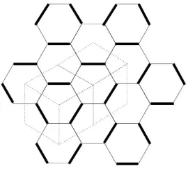
x+y+z= 0). To see that every such tiling gives rise to a dimer cover of a portion of the honeycomb lattice, proceed as follows: call all left-pointing triangles in the lattice black and all right-pointing ones white, and for each rhombus present in the tiling, draw a line between the centroid of its black triangle and the centroid of its white triangle. This will give a matching of the dual graph (whose vertices consist of all the centroids). Each edge in this matching joins a black vertex (triangle) to a white one. See Figure3.2.

a

=

N

[image:32.612.141.430.189.329.2]

c

=

S

b

=

T

−

S

Figure 3.1: A tiling of a 3×2×3 hexagon and the associated stepped surface.

Figure 3.2: Duality between tilings and matchings, as appears in [Ken97] (figure used with permission).

A yet different way of viewing such tilings, important hereinafter, is as collections of nonintersect-ing paths in the square lattice. The paths start at consecutive points on the vertical axis (countnonintersect-ing from the origin upwards) and end at consecutive points on a vertical line with displacement b+c

from the origin. Each path is composed of horizontal segments or diagonal (southwest to northeast, slope 1) segments, and the paths are required not to intersect. Given any such collection of paths, we can recover a hexagonal tiling (and hence a dimer cover) from it and vice versa. For reasons that will become clear as we progress, we will find it more convenient to encode the hexagon via the following three numbers:

[image:32.612.220.355.386.509.2]

(33)

Figure3.3explains the above, and also introduces two coordinate systems useful later on: Carte-sian coordinates (i, j) for the hexagon picture and (t, x) for the nonintersecting paths in the square lattice picture. They are related by

(i, j) = (t, x₋t/2).

j

i j

i x

[image:33.612.116.537.131.287.2]

t

Figure 3.3: Duality between tilings and nonintersecting paths.

Following the notation in [BG09], let Ω(N, S, T) denote the set ofN nonintersecting paths in the lattice _N2 _{starting from positions (0}_,₀₎_{, . . . ,}₍₀_{, N}

−1) and ending at positions (T, S), . . . ,(T, S+

N₋1). Each path has segments of slope 0 or 1 (as explained above). Set

XS,t_N,T =_{x_∈Z: max(0, t+S−T)≤x≤min(t+N−1, S+N−1)},

XN,TS,t ={X = (x1, . . . , xN)∈(X S,t N,T)

N _:_x

1< x2<· · ·< xN}.

XS,t_N,T is the set of all possible particle positions in a section vertical section of our hexagon with horizontal coordinatet(in (t, x) coordinates). XN,TS,t is the set of all possibleN-tuples of particles in

the same vertical section.

For X _∈ Ω(N, S, T), we have X = (X(t))0≤t≤T and each X(t) ∈ X_N,TS,t . X is a discrete time

Markov chain as it will be shown.

To any dimer cover of a planar bipartite graph one can associate a height, which is a function from dimer covers to (usually real, often rational) numbers. While we could do this in general-ity, we restrict attention to lozenge tilings of the hexagon (and the associated dimer covers). We want to formalize the three-dimensional “height” one sees in Figure 3.1. We will be skipping most homological details, trivial as they may be in the case of bipartite planar graphs.

(34)

byd∗(ω)(v) =P

eω(e) whereω is a flow and the sum is over all edges incident at v. This map is

called the divergence. Ifd∗(ω)(v) is positive (negative), we sayv is a source (sink) for the flowω. Given a dimer cover M ofG, we associate the flow ωM as follows: ωM(e= (b, w)) = 1 if (b, w)

is an (oriented black to white) edge present in the cover, and ω(e) = 0 ife is not inM. This flow has divergence +1 (₋1) at black (white) vertices. For M1, M2 dimer covers of G, ωM1−ωM2 is

divergence free.

Given a divergence free flowωonGand a reference (fixed) facef0, one defines a height function

h on all other faces as follows. First h(f0) = 0 (hence the name). For any other face f, pick a path p in the dual graph from f0 to f. We define h(f) as the net (signed sum) flow of p as it crosses the edges ofGwith the caveat that aspcrosses an unoriented edgee, we add to the sum the contribution w(e: oriented left to right). his independent of the path pchosen in the dual graph sinceωis divergence free.

For G we can fix a base flow ω0 with divergence 1 (-1) at black (white) vertices. GivenM a dimer cover, we can construct the flowωM as above. Choosing a reference facef0, we can associate

to the difference flow (which is divergence free) a height functionhM as in the previous paragraph.

We call it theheight of the dimer cover (equivalently, of the lozenge tiling for the case of honeycomb dimers).

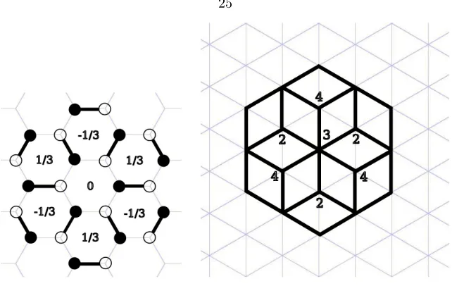
For the lozenge tilings dual to honeycomb dimers we are interested in, a natural base flowω0 is defined byω0(e= (b, w)) = 1/3 where the edge (b, w) comes with black to white orientation. In this case, for a given dimer coverM, the heighthM is (up to an additive constant), when evaluated at

the center of a face, the distance between that center and the planex+y+z= 0 when we interpret

M as a stepped surface. See Figure3.4where on the left we exhibit the height of the dimer cover and on the right, the distance (multiplied by√3) from the interior vertices of the tiling to the plane

x+y+z= 0.

3.2 Kasteleyn theory

Given a bipartite planar graph G = (V, E) that has dimer covers (in particular, if G is finite, V

needs to be even), we can attach various weightsw:E_→_Cto its edges. We can then consider the following Boltzmann measure on dimer coversM ofG:

µ(M) = 1

Z

Y

e∈M

w(E), (3.2.1)

where Z = P

M

Q

e∈Mw(E) is the partition function. We will talk about probability measures

hereinafter, so we wantµto take positive real values between 0 and 1 (this does not mean that w

(35)

[image:35.612.164.485.57.260.2]

Figure 3.4: The height function on a matching (left) and on a stepped surface/lozenge tiling (multiplied by√3).

change the functionwby multiplying weights of all edges incident to a single vertexuby a number

c. Then both Z and the numerator in (3.2.1) will get multiplied by c (because in the sum over all matchings, the vertex uis going to be matched, so c will multiply every term in the partition function, as well as the denominator). Therefore, the measure µ will not change, though we are looking at a new Boltzmann weightw0. We call two such weightsgauge equivalent if they differ by a finite number of such multiplications.

There is a simple criterion (see, e.g.,[Ken09]) to test whether two weightswandw0 on the graph are gauge equivalent: they are so if and only if for every face bounded by edges e1, . . . , e2k (listed

consecutively; note every face has an even number of edges due to the bipartite structure), we have

w(e1)w(e3). . . w(e2k−1) w(e2)w(e4). . . w(e2k)

=w

0₍_e₁₎_w0₍_e₃₎_{. . . w}0₍_e

2k−1) w0₍_e

2)w0(e4). . . w0(e2k) .

We will now define a Kasteleyn sign weight on the graph G. It is a choice of signs assigned to every edge such that each face with 0 mod 4 edges around it has an odd number of₋signs around it, and each face bounded by 2 mod 4 edges has an even number of minus signs around it. Note for dimers of the honeycomb graph (or parts of it), there is a very convenient choice of Kasteleyn weight coming from the fact that 6 = 2 mod 4: just put a + sign on every edge. This is the only case we will be interested in the present work, but in general one can prove existence of such weights via spanning trees (see [Kas67] and [TF61]).

TheKasteleyn matrix K associated to a planar bipartite graphGwhose vertex setV =B_∪W

(36)

for the Kasteleyn sign weight.

We have the following theorem from [Kas67], [TF61] for computing the partition functionZ(the total weight of all matchings). SetG(V, E) to be a finite bipartite planar graph with an even number of edges such thatV =B_∪W.

Theorem 3.2.1.

Z =_|detK_|.

Proof. We will only prove this for the honeycomb lattice, in which case the proof simplifies a lot. We follow [Ken09]. We first expand the determinant as

detK= X

σ∈Sn

(₋1)σK(b1, wσ(1)). . . K(bn, wσ(n)).

Notice each term in the above sum is 0 unless each vertex bi in the product is paired with an

adjacentwσi. Hence for each dimer cover we find a nonzero term in the sum and vice versa. The

summand in question is indeed the total weight of that dimer cover by definition.

So all there is to check is that all signs appearing in front of the nonzero terms are the same. It suffices to show that given a reference cover (a choice of σ), all other covers are obtained my multiplyingσby even permutations. But this can be translated into the tiling picture of Figure3.1 bijectively. There, it is easy to see that we can get from any tiling to any other tiling by changing unit cubes, one at a time, from empty to full (or vice versa). In particular we can reach any tiling from the empty box tiling with such moves. But every such move is local, on a unit cube alone. Such empty/full (or full/empty) swap corresponds to swapping the two dimer covers of a hexagonal in the honeycomb lattice - a 2π/3 rotation. It corresponds to multiplying the initial permutationσ

(corresponding to the initial cover) by a 3-cycle - an even permutation. Hence all the terms in the sum have the same sign as the term corresponding to the empty tiling (being obtained from it by multiplying the “empty”σby even permutations). This concludes the proof.

The next theorem, due to Kenyon [Ken97] will allow us to compute total weight of all matchings containing certain prescribed edges. We will omit the proof but see the reference (the proof uses the Jacobi lemma relating minors of a matrix with its inverse).

Theorem 3.2.2. The total weight of matchings containing n fixed edges (b1, w1), . . . ,(bn, wn) is

equal to

n

Y

i=1

K(bi, wi)

!

det 1≤i,j≤nK

−1₍_w

i, bj).

A version of this theorem which we find useful in computations is the following.

Theorem 3.2.3. The total weight of matchings of the graphG0which is obtained fromGby removing

(37)

of bi andwj:

det 1≤i,j≤nK

−1₍_w

i, bj).

Remark 3.2.4. Theorem3.2.2can be deduced from3.2.3since fixing certain edges in a matching is equivalent to removing the corresponding vertices, computing the total weight, and then adding the vertices back in the matching with prescribed edges (in which case we have to multiply by the weights of those edges).

Remark 3.2.5. Both of the previous theorems follow from the Jacobi lemma relating minors of a matrix M with those of its inverse. Let M be nonsingular and Adj(M) (the adjugate of M) be defined by Adj(M)i,j = (−1)i+jMˆ_j,ˆ_i where Mˆ_i,ˆ_j is the determinant of the matrix obtained by removing the i-th row and j-th column from M. Then M_i,j−1 = _det1_MAdj(M)i,j. In fact, more

is true: any k_×k minor in Adj(M) is equal to the complementary signed minor in MT (the transpose ofM) times (detM)k−1. As a corollary, ifN0 is a proper square submatrix ofM−1, then

|detN0_|₌_|_det_N_|_/_|_det_M_|_{for some proper square submatrix}_N _of_M_.

For the honeycomb graph, we can enumerate matchings differently. We look at the associated tiling, and then at the associated collection of nonintersecting paths. The total weight of all noninter-secting path collections (equivalently, all dimer covers) is then given by the Lindstr¨om-Gessel-Viennot lemma, which we now state in more generality (see [Ste90] and references therein):

Theorem 3.2.6. For a planar weighted connected graph G, let (u1, . . . , un) be a tuple of starting

points and(v1, . . . , vn)be a tuple of ending points. Assume there are no nonintersecting path

collec-tions pairing (start-end) ui tovσi for a nontrivial σ∈Sn. Moreover, letT(u, v) be the total weight

of all paths fromutov in the graph (the weight of one path is the product of the edge weights over

edges in the path). Then the total weight of all nonintersecting paths from the starting tuple to the

ending one such that the i-th path starts atui and ends atvi is:

det

1≤i≤nT(ui, vj).

3.3 Elliptic measure on tilings and canonical coordinates

We will now define the (Boltzmann) probability measure on Ω(N, S, T) (equivalently, on tilings of the

a_×b_×chexagon) that will be the object of study. For a tilingTcorresponding to anX_∈Ω(N, S, T) we define its weight to be

w(T) = Y

(38)

where by a horizontal lozenge we mean a lozenge whose diagonals are parallel to the iand j axes. The probability of such a tiling would then simply be

P rob(T) = P w(T)

S∈Ω(N,S,T)w(S)

.

The weight functionwon horizontal lozengesl is defined by

w(l) :=w(i, j) = (u1u2)

1/2_qj−1/2_θ

p(q2j−1u1u2)

θp(qj−3i/2−1u1, qj−3i/2u1, qj+3i/2−1u2, qj+3i/2u2) = (v1v2)

1/2_qj−S/2−1/2_θ

p(q2j−S−1v1v2)

θp(qj−3i/2−S−1v1, qj−3i/2−Sv1, qj+3i/2−1v2, qj+3i/2v2)

,

(3.3.1)

where (i, j) is the coordinate of the top vertex of the horizontal lozengel, u1, u2, q, p are complex parameters (_|p_|<1) andu1=q−Sv1, u2=v2(the reason for thev parameters is that this break in symmetry will make other formulas throughout the thesis more symmetric).

Remark 3.3.1. Only considering weights of horizontal lozenges for a tiling of a hexagon is equivalent to considering all types of lozenges but assigning the other two types weight 1 (i.e., each lozenge that is not horizontal has weight 1). This is a break in symmetry that can easily be fixed. However, for most computations in this Chapter and next we prefer this non-symmetric weight assignment system as it makes some things easier. Nevertheless, we show in Section 3.8 that we can assign weights to the 3 types of lozenges in anS3-invariant way (i.e., invariant under permuting the 3 types of lozenges or equivalently the 3 spatial directions) by changing gauge.

This weight on dimer coverings of a hexagon was derived in [BGR10] (see also [Sch07] for the nonintersecting paths derivation), and the derivation will be sketched in Section3.6.

The connection with elliptic functions will now be explained. Fix a horizontal coordinate i, denote byw(i, j) the weight of the horizontal lozenge with top vertex coordinates (i, j), and observe that for two consecutive vertical positions we have (u1u2u3= 1):

r(i, j) = w(i, j+ 1)

w(i, j) =

q3_θ

p(qj−3i/2−1u1, qj+3i/2−1u2, q−2j−1u3)

θp(qj−3i/2+1u1, qj+3i/2+1u2, q−2j+1u3) = q

3_θ

p(qj−3i/2−S−1v1, qj+3i/2−1v2, q−2j+S−1/v1v2)

θp(qj−3i/2−S+1v1, qj+3i/2+1v2, q−2j+S+1/v1v2)

.

(3.3.2)

In the three-dimensional coordinates (x, y, z) pictured in Figure3.5(note we only consider sur-faces in 3 dimensions that arestepped, meaning there is a one to one correspondence between the two-dimensional tiling picture and the three-two-dimensional surface picture) withi=x₋y, j=z₋(x+y)/2 (after shifting (i, j) so that origin is at the hidden corner of the box), the weight ratio is equal to:

r(x, y, z) = w(full box)

w(empty box) =

q3_θ

p(˜u1/q,u˜2/q,u˜3/q)

θp(˜u1q,u˜2q,u˜3q)

(39)

j

i

z

[image:39.612.266.382.53.187.2]

y x

Figure 3.5: Going from 3 dimensions to 2 dimensions.

Figure 3.6: A full 1×1×1 box (left) and an empty one (right).

where

˜

u1=qy+z−2xu1, u˜2=qx+z−2yu2,u˜3=qx+y−2zu3, u1u2u3= 1,

and (x, y, z) is the three-dimensional centroid of the 1_×1_×1 full cube (on the left in Figure3.6) with top lid the horizontal lozenge having top vertex coordinate (i, j).

The word elliptic now becomes clear asr in (3.3.3) is an elliptic function ofq (that is, defined on_E—see the Introduction for details). Moreover, ris the unique elliptic function of q with zeros at ˜u1,u˜2,u˜3 and poles at 1/u˜1,1/u˜2,1/u˜3 normalized such thatr(1) = 1. Of interest is also that r is elliptic in ˜uk fork= 1,2,3 subject to the condition thatQ3_k₌₁u˜k= 1.

Remark 3.3.2. The above paragraph can be restated by observing we can build everything by choosing 3 pointsq, u1, u2 on the elliptic curveE.

Remark 3.3.3. The weight ratio ris invariant under the natural action ofS3permuting the ˜uk’s

(and of course the 3 axes: x, y, z).

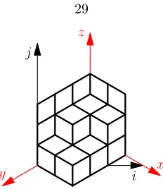
We can view our tilings as stepped surfaces composed of 1_×1_×1 cubes bounded by the 6 planes

x = 0, y = 0, z = 0, x = b, y = c, z =a. Then the two-dimensional picture in Figure 3.1 can be viewed as a projection of the 3 dimensional stepped surface onto the planex+y+z= 0.

ForT a tiling, we have

wt(T) = Y

∈T w(i, j),

(40)

cubes into columns in thezdirection with fixed (x, y) coordinates (see Figure3.5), we obtain

wt(T) =const_·Yw(i, j+ 1) w(i, j) ,

where the product is taken over all cubes (visible and hidden) of the boxed plane partition and (i, j) is the top coordinate of the bounding hexagon of a 1_×1_×1 cube. Note to get to this equality we have merely observed that wt(empty box) is a constant independent of i and j. We can further refine this (rearranging the terms in the product and gauging away more constants—see Section 2.3 of [BGR10] and also Section 3.1above for more details) as

wt(T) =const_·Y v

_w₍_{i, j}_{+ 1)}

w(i, j)

h(v)

=const_·Y v

r(i, j)h(v),

where v= (x0, y0, z0) ranges over all vertices on the border (but not on the bounding hexagon) of the stepped surface withx0, y0, z0 integers (equivalently,v ranges over all vertices of the triangular lattice inside the hexagon, but we viewvin 3 dimensions). h(v) is the distance fromvto the plane

x+y+z= 0 divided by√3 : h(v) = (x0+y0+z0)/3.

For the remainder of the section, we will discuss the concept of canonical coordinates for the geometry of elliptic tilings. That is, it will be convenient for various computations to express the geometry of an elliptic lozenge tiling in terms of coordinates on a certain product of elliptic curves. First we will introduce 6 parametersA, B, C, D, E, F depending onq, t, S, T, N, v1, v2(note we have listed, other than q, 6 parameters, of which 4 are discrete and dictate the geometry: t, S, T, N). t

here is a (discrete) time parameter and ranges from 0 toT. It will be explained better in Chapter4. It corresponds to the fact that we will be interested in distributions of particles on a certain vertical line: that is, tilings of hexagons that have prescribed positions of particles (or holes) on the vertical line with horizontal coordinatet.

The set of parameters of interest to us is

A=qt/2+S/2−T+1/2√v1v2, B =qt/2+S/2+T+1/2

r_v

2

v1

,

C=qt/2−S/2−N+1/2_√1 v1v2

, D=q−t/2+S/2−N+1/2_√1 v1v2

, (3.3.4)

E=q−t/2−S/2+1/2

r_v

1

v2

, F =q−t/2−S/2+1/2√v1v2.

Observe that they satisfy a certain balancing condition (like the one in Section 2.3):

Elliptic Combinatorics and Markov Processes