M E T H O D O L O G Y A R T I C L E
Open Access
Probabilistic models for CRISPR spacer content
evolution
Anne Kupczok
*and Jonathan P Bollback
Abstract
Background: The CRISPR/Cas system is known to act as an adaptive and heritable immune system in Eubacteria and
Archaea. Immunity is encoded in an array of spacer sequences. Each spacer can provide specific immunity to invasive elements that carry the same or a similar sequence. Even in closely related strains, spacer content is very dynamic and evolves quickly. Standard models of nucleotide evolution cannot be applied to quantify its rate of change since processes other than single nucleotide changes determine its evolution.
Methods: We present probabilistic models that are specific for spacer content evolution. They account for the
different processes of insertion and deletion. Insertions can be constrained to occur on one end only or are allowed to occur throughout the array. One deletion event can affect one spacer or a whole fragment of adjacent spacers. Parameters of the underlying models are estimated for a pair of arrays by maximum likelihood using explicit ancestor enumeration.
Results: Simulations show that parameters are well estimated on average under the models presented here. There is
a bias in the rate estimation when including fragment deletions. The models also estimate times between pairs of strains. But with increasing time, spacer overlap goes to zero, and thus there is an upper bound on the distance that can be estimated. Spacer content similarities are displayed in a distance based phylogeny using the estimated times. We use the presented models to analyze differentYersinia pestisdata sets and find that the results among them are largely congruent. The models also capture the variation in diversity of spacers among the data sets. A comparison of spacer-based phylogenies and Cas gene phylogenies shows that they resolve very different time scales for this data set.
Conclusions: The simulations and data analyses show that the presented models are useful for quantifying spacer
content evolution and for displaying spacer content similarities of closely related strains in a phylogeny. This allows for comparisons of different CRISPR arrays or for comparisons between CRISPR arrays and nucleotide substitution rates.
Keywords: CRISPR/Cas, Maximum Likelihood, Microbial genome evolution, Bacterial immunity
Background
Bacteria and Archaea have an adaptive heritable immune system against viruses, plasmids and other mobile genetic elements [1,2]. This locus, CRISPR (Clustered Regularly Interspaced Short Palindromic Repeats), consists of an array of repeats and unique spacers. The repeats are of length 21-48 nucleotides depending on CRISPR type and species. The spacer sequences are 26-72 nucleotides in length, where the variance of spacer length within one array is small. The spacer sequences were found to be of
*Correspondence: [email protected]
IST Austria (Institute of Science and Technology Austria), Am Campus 1, A-3400 Klosterneuburg, Austria
extrachromosomal origin [3] and are involved in immu-nity [1,2]. Cas (CRISPR-associated) genes adjacent to the CRISPR arrays are necessary for the biogenesis of the CRISPR RNA, for the interference with the target nucleic acid and for the acquisition of new spacer sequences [4]. Different types of CRISPR/Cas systems exist based on the set of Cas genes present [5].
Comparisons of the CRISPR array of closely related strains showed that the CRISPR array undergoes a rapid evolution that is mainly determined by the gain and loss of the whole system or of individual spacers [6,7]. In most cases, spacer addition was observed at the begin-ning, the ‘leader’ end, of the array [1] and the pattern in
metagenomic samples suggest that deletion of consecu-tive repeat-spacer units occurs [6]. Bacterial genomes can have multiple CRISPR arrays that differ in their dynamics [7-9]. It was observed that closely related strains can differ in their spacer content, thus the CRISPR array is used as a tool for strain typing (e.g., [8,10,11]).
The targeting of extrachromosomal elements by the CRISPR/Cas system was discovered recently [1,2] and many questions regarding the functions, mechanisms and evolution of this locus are still open. This is complicated by the fact that different CRISPR/Cas systems have dif-ferent mechanisms and may have difdif-ferent function [4]. Thus computational methods that make predictions are important to narrow the space of hypotheses that need to be tested experimentally. For example, self-targeting spac-ers are not conserved between species and CRISPR arrays with self-targeting spacers may get inactivated. These observations exclude the hypothesis of gene regulation by CRISPR [12].
Using model simulations can provide insights into the parameters allowing CRISPR existence and into the details of CRISPR dynamics. One result using population genet-ics models is that CRISPR is maintained if it provides immunity to viruses or plasmids even when there is a cost of having CRISPR [13]. Simulating a spatial model of virus and host population showed that coexistence is possible with a CRISPR-based immune system [14]. Furthermore, a spatially structured environment can lead to interme-diate array lengths, i.e., the number of spacers has an optimum between 0 and the number of viruses excluding the extreme values. Then the lengths are determined by the spacer insertion rate and by the cost for having spac-ers not by the total number of phages in the environment [15]. Modeling coevolution of hosts and viruses results in the observation that spacers at the leader-distal end tend to be more conserved, due to selective sweeps, and that immunity to contemporary viruses is mainly determined by the most recently acquired spacers [16,17]. In addition, simulations can find parameter regimes that are impor-tant for the existence of CRISPR like a threshold on the viral mutation rate [18].
Our approach differs from the population genetics mod-els described since itestimatesparameters directly from the array data. We describe the dynamics of the CRISPR locus over time in diverging populations related by a phy-logeny. This is the phylogeny of the CRISPR/Cas locus. Since the locus can be transferred horizontally [19], the CRISPR/Cas phylogeny does not need to be identical to the strain phylogeny. There are a few instances of recombination inside cas genes [20], but in our model, we exclude recombination in the spacer arrays. The evolutionary events we model are spacer insertion and deletion. By using only strains harboring the locus, we ignore the loss or gain of the whole CRISPR/Cas system.
Mutations inside the CRISPR locus are also not included in the model, but in data analyses multiple spacers with sequence similarities can be subsumed into one identity.
Even before the function of the CRISPR/Cas system was clear, Pourcel et al. [8] formulated three observations for CRISPR evolution by comparing Yersinia pestis arrays: Random deletions of one or more spacers and repeats; polarized addition of new spacers; and identical spacers reflect shared ancestry not independent events. We also assume that the CRISPR arrays analyzed are homologous and that each spacer was only inserted once, i.e., all spac-ers with identical sequence are identical by descent. Thus we present three models: an unordered model (spacer content is considered as a set), an ordered model (where insertion is polarized, i.e., insertions occur at one end only) and a fragment loss model (where insertion is polar-ized and successive spacers can get deleted together in a single event).
Another class of models that take order relationships into account are gene order models, i.e., they model the order of genes in the genome over time. Most methods for evaluating the distance between two gene orders find the minimum number of rearrangement events between these genomes. This approach can also be combined with insertions and segment deletions [21,22]. Probabilistic methods of rearrangement only model inversions [23,24] or inversions and transpositions [25]. Multi-gene events are considered in one model of gene innovation, duplica-tion and deleduplica-tion, but ignoring the order of genes on the genome [26].
Our ordered and fragment loss models are thus differ-ent from the probabilistic models for gene order since they capture the properties specific for CRISPR spacer evolution. We describe our method and investigate its properties by simulation and application to real world
Yersinia pestisdata sets [8,27].
Methods
Models
We describe different models for estimating insertion and deletion rates from CRISPR arrays. We ignore repeats and only use the spacer information and their order encoded in an array. The leader end is displayed on the left (see also Figure 1). In our models, these arrays evolve by insertion and deletion events. An overview of the types of insertions and deletions allowed in the different models can be found in Table 1. In all models, the waiting time for insertion events is exponentially distributed with rateλ(Figure 1). One spacer is inserted for each insertion event.
In theindependent loss modelonly single spacers can get lost. For each spacer, the waiting time to get lost is expo-nentially distributed with rateμ. All deletions are inde-pendent of each other. The correspondinglength model
3 2 1
4
3 2 1
3 2
3 1
2 1
3
[image:3.595.58.290.89.256.2]1
[image:3.595.305.541.89.237.2]Figure 1Illustration of the instantaneous rates for an array of length 3.Leader-proximal end is on the left. The arrows display the allowed transitions for the fragment loss model. Deletions of length two are are displayed in red, deletions of length three in green. For the independent loss model, only the black arrows are allowed transitions. For the unordered model, the transition with rateλresults in either 4-3-2-1, 3-4-2-1, 3-2-4-1 or 3-2-1-4 with uniform probabilities.
(Figure 2). In contrast, thefull modeltakes spacer iden-tities into account. In the independent loss model, a loss means a transition to length−1 and a gain a transition to length+1. We analyze two sub-models of the independent loss model: theunorderedmodel, where there is no posi-tion informaposi-tion; and theordered model, where insertion occurs in a polarized way, i.e., at the end adjacent to the leader. For simplicity, we refer to this end as thebeginning
of the array. The latter model is motivated by the observa-tion that spacers are usually inserted at the leader end of the array (e.g., [1]).
In thefragment loss model the position is informative since insertion occurs in the beginning and subsequent spacers can get lost together. This model is motivated by the pattern in metagenomic samples that shows deletion of consecutive repeat-spacer units [6]. Each possible non-empty substring of the array is a fragment. Thus fragments can be overlapping and one spacer inside an array is then part of different fragments. For example, the array 3-2-1 (Figure 1) consists of the fragments 1, 2, 3, 2-1, 2 and 3-2-1. The fragment 3-2 overlaps with the fragment 2-1 in the spacer 2. And the spacer 2 occurs in 4 fragments: 2, 2-1, 3-2 and 3-2-1. For each possible fragment, the wait-ing time to get lost is exponentially distributed with rate
Table 1 Overview over models
Independent loss model Fragment loss model
Unordered Ordered
Insertions Random Polarized Polarized
Deletions Single Single Fragments
A
0
1
2
3
B
[image:3.595.57.292.674.733.2]0
1
2
3
Figure 2Markov chain representation of the length models. (A) Independent loss model. (B) Fragment loss model. For clarity, deletions of length 2 are red, deletions of length 3 are green, and deletions≥4 are not displayed.
μ, independent of the number of spacers a fragment con-tains. In the length model, all lengths smaller than the current length are accessible in a single step (Figure 2).
Since μ has a different meaning in both models, we emphasize this by usingμF for the fragment loss model (μF affects each possible fragment), andμI for the inde-pendent loss model (μI affects only single spacers). The rates are always rescaled such that one event (insertion or deletion) is expected in timet = 1. This allows for
esti-mating times, but only the ratioρ = λ
μcan be estimated.
Again, we distinguish the two models by usingρF = μλ F
andρI= λ
μI
. Subscripts are omitted when the underlying
model is clearly stated.
Now, we present the stationary distribution of the length models and the transition probabilities of the full model necessary to formulate an estimation approach under each of these models. Afterwards details of the estimation approaches are described.
Independent loss models
Length model The independent loss length model is a Markov process known as an M/M/∞ queuing model [28] (Figure 2A). In this queuing model, customers (i.e., spacers) arrive according to a Poisson process with rate λ. They are immediately served and exit after an exponential waiting time with rateμ. The stationary dis-tribution of the number of busy servers (i.e., the number of spacers in the array), is a Poisson distribution with rateρ:
p(n|ρ)=e−ρρ
n
0 5 10 15
0.00
0
.10
0.20
Length
Frequency
ρI=2.4
ρF=10
ρI=4.8
ρF=50
ρI=6.4
[image:4.595.60.540.86.242.2]ρF=100
Figure 3Stationary distribution of the length models.Subscript I represents the independent loss model and subscript F the fragment loss model.ρs of the same color result in the same mean length, i.e., they are correspondingρs.
Transition probabilities Given an ancestor s0 and a
descendents1,mspacers are shared,dspacers are unique
tos0andjspacers are unique tos1. The transition
prob-abilities of changing froms0tos1 use the property that
inserted, preserved and deleted elements are independent of each other:
T(s0→s1|t,λ,μ)=M(m|t,μ)D(d|t,μ)I(j|t,λ,μ)
Where the probability of preservingmspacers in time
tisM(m|t,μ)=e−mμt,
the probability of loosingdspacers in timetis
D(d|t,μ)=(1−e−μt)d,
the probability of insertingjspacers in timetis
I(j|t,λ,μ)= e
−ρ(1−e−μt)
ρ1−e−μtj
j! .
(2)
M andDfollow directly from the exponential model.
I is known from queuing theory [28]. The probability of insertingjspacers is the probability of observingjspacers after timetwhen there were 0 spacers at time 0. That is the integration over all possible paths leading toj, includ-ing paths where spacers were inserted and lost and thus never observed.
Fragment loss models
Length model The stationary distribution of the length model (Figure 2B) is given by
p(n|ρ)= (n+1)(n+2)
2ρn i=0(
(i+1)(i+2)
2ρ +1)
. (3)
Equation (3) can be solved from the conditions that in stationarity the flow into a state equals the flow out of that
state and that the probabilities of such events necessarily sum to 1 (see Additional file 1).
For eachρFthere is acorrespondingρIthat has the same expected length. We find that for corresponding ρs the fragment loss model has a higher variance of the length distribution than the independent loss model (Figure 3).
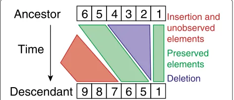
Transition probabilities Given an ancestor s0 and a
descendents1, we segment them into independent pairs
(Figure 4). Note that this segmentation is different from the fragments described above. Fragments are all possible substrings of one array, but segments are calculated using two arrays. Each segment is either an inserted, deleted or preserved segment. Segments are of maximal length, i.e., two consecutive segments are of different type. See Figure 4 for an example of segments resulting from a pair of arrays. In contrast to the independent loss model, this segmentation is an approximation since it ignores the probability of deletion events spanning multiple seg-ments. The segmentation is, however, necessary to factor-ize the transition probabilities. The transition probability is then the product over the segment probabilities.
6
5
4
3
2
1
7
6
1
9 8
5
Insertion and unobserved elements
Deletion
Preserved elements
Ancestor
Descendant
Time
[image:4.595.304.540.581.682.2]Preserving a fragment of lengthmhas probability
M(m|t,μ)=e−m(m2+1)μt.
Deleting a fragment of any length has probability
D(t,μ)=1−e−μt.
Insertingispacers has probability
I(i|t,λ,μ)=2i+1e−λtρi
× i+1
k=1
(−1)k−1 (1+2k)k(k+1) 2(i−k+1)!(i+k+2)!
× e −k(k+1)
2 μt
1− (i+2)(i+21ρ)−(k+1)k
1+ k(k2+ρ1) )
⎤ ⎦
+ (i+1)(i+2) 2ρ
i
k=0
(k+1)(k+2)
2ρ +1
.
(4)
As before, the probability of insertingispacers includes unobserved spacers that were inserted and lost again. These equations were found by integration over all possi-ble paths in Mathematica 8.0 [29].
For example, in Figure 4 the transition probability is
I(3|t,λ,μ)×M(2|t,μ)×D(t,μ)×M(1|t,μ).
Estimation
Maximum likelihood function
We describe a maximum likelihood approach to estimate rates and times of spacer insertions and deletions, given a set of ordered spacer arrays from different strains. Since we do not have phylogenetic information, we consider each pair of arrays and their possible common ancestors.
Formally, the maximum likelihood estimate for a spacer setSwith k=|S|is
(ρˆ,ˆt)=argmaxL(ρ,t|S)withL(ρ,t|S)= i=1,...,(k2)
L(ρ,ti|si),
(5)
where sis the list of all different pairs of S andt is the corresponding list of pairs of times.
The likelihood of a pair of spacer arrays (s1,s2) with
times(t1,t2)is then
L(ρ,t1,t2|s1,s2)=
ancestorsa
q(a|λ,μ)T(a→s1|t1,λ,μ)
×T(a→s2|t2,λ,μ),
(6)
whereλandμare computed fromρgiven the constraints
λ
μ = ρand the expected number of insertions and
dele-tions in time 1 is 1. Then,q(a|λ,μ)is the probability of observinga,T(a→b|t,λ,μ)is the transition probability
of changing fromatobin timetgiven insertion rateλand deletion rateμ.
If the pair has no overlap, i.e., no common spacers, we assume that the time from the common ancestor is long enough such that the transition probabilities approach the stationary probabilities. Then the likelihood function can be simplified by using the fact that the probability of the whole ancestor space is 1. We find that only the lengths are informative for estimatingρ:
L(λ,μ|s1,s2)=
ancestorsa
q(a|λ,μ)p(n1|ρ)p(n2|ρ)
=p(n1|ρ)p(n2|ρ), withn1=|s1|andn2=|s2|.
(7)
Note thatqandpare different but related by the following constraints: The sum of allq(a)with|a| = nisp(n)and
q(a)=q(b)if|a| = |b|.
Optimization
We are interested in both the estimate of ρ, ρˆ, and the estimation of the divergence times. For a pair, we denote the estimated time between two arrays asτˆ= ˆt1+ˆt2.τfor
a phylogeny or for a collection of pairs denotes the average ofτ over all pairs.
Overview of the estimation approach:
1. Estimate a startingρfrom the length model by
maximum likelihood. The likelihood function is
Lstart(ρ)= arrayssp(|
s| |ρ), where|s|is the length ofs
andp is the stationary distribution of the length
model.
2. For each pair of spacers with overlap, generate the possible ancestors: Ancestral arrays can be arbitrarily large, but the probability of observing a certain
length is given byp(n). For practical reasons we do
not consider ancestors whose length is outside the
central 99% of the stationary distribution given byρ
estimated in step 1, since they would have a
negligible contribution to the likelihood. In detail, the
lengthl1where the cumulative distribution exceeds
0.005 is the minimum ancestor length and the length
l2where the cumulative distribution exceeds 0.995 is
the maximum ancestor length. Then the possible
ancestor lengthsn are betweenl1andl2:l1≤n≤l2.
3. (a) For all pairs with overlap, estimate the times
with fixedρ. It is possible to iterate through
the pairs and estimate their times independently of the other pairs. The estimation of both times is iterated alternatingly until the likelihood has converged.
(c) Check if the log-likelihood of the estimated parameters has converged, then return the estimated parameters, else repeat step (a) with the new parameters.
All three models are analyzed in this computational framework. All optimization steps only optimize one parameter and use Powell’s method from the python pack-age scipy [30]. The python package mpmath is used for high-precision computing [31] that is necessary to compute the probability functions accurately.
Ancestors
Here, we describe for each of the models how we generate the ancestors in step 2 above. Thereby we must account for unobserved spacers, that are not present in the data but in ancestral lineages. We overcome the problem of the infinite state space by ignoring the identity of unobserved spacers. For example, there may be four unobserved spac-ers, each of them gets a new unique name, but then no other four unobserved spacers with other names or an other order are considered.
Unordered model Given a pair of arrayss1ands2, they
havecspacers in common,d1are unique tos1andd2are
unique tos2. Then allnbetween min(c,l1)andl2are
gen-erated. When lengthnis generated, enumerate alli, j, u
such thatc+i+j+u =n,i ≤d1andj ≤d2. Then for
ancestora, there areccommon spacers,ionly occur ins1,j
only occur ins2anduare unobserved (they are lost in both
lineages). Since this ancestor comprises multiple spacer identities, we assign a weight to it, w(a) = d1i× d2j. The weights for eachnare rescaled such that they sum to 1, i.e., the rescaled weightwsisws(a) = w(a)
b,|b|=|a|w(b)
. Then
q(a)=ws(a)p(|a|).
Ordered model Given a pair of arrayss1ands2, find the
first shared spacer. The ancestor must contain this spacer and all subsequent spacers from both arrays, these arec
spacers in total. There ared1 andd2spacers before the
first shared spacer in s1 ands2, respectively. With these
new definitions of c, d1 and d2, the method from the
unordered model is applied.
Fragment loss model For the fragment loss model, the ancestors must fulfil several constraints given by the order in the observed arrays. Since all shared ancestors are iden-tical by descent and insertions occurs only in the begin-ning, all spacers from the first shared spacer on must be present in the ancestor. Thereby the order of spacers must be preserved. Enumerating the ancestors is best explained with an example. Consider the arrayss1 =8-7-6-4-3-2-1, s2=11-10-9-7-6-5-2.
• 7 is the first shared spacer.
• The set of spacers necessarily present in the ancestor
is the union of all spacers after the first shared spacer:
{1, 2, 3, 4, 5, 6, 7}.
– Possible orders of these spacers:
7-6-5-4-3-2-1, 7-6-4-5-3-2-1, or 7-6-4-3-5-2-1
• The set of spacers possibly present in the ancestor is
the union of all spacers before the first shared spacer:
{8, 9, 10, 11}.
– Order constraints for these spacers: 11 before 10 before 9 before 7
• Unobserved spacers (spacers present in the ancestor
and lost in both lineages) may have occurred at all possible positions.
Since a lot of possible arrays are generated by this approach, heuristics are used to reduce their number:
• Shared fragments cannot be interrupted by an
unobserved spacer.
– In the example, there is no unobserved spacer between 6 and 7.
• Unique fragments in the beginning are not mixed.
– In the example, 8 and 11-10-9 are in the beginning and then the following ancestral fragments are not allowed: 11-8-10 and 10-8-9.
• Deleted pairs are also not mixed.
– In the example 4-3 and 5 are deleted and the ancestral fragment 4-5-3 is ignored.
• The number of positions with unobserved spacers is
maximal four. That means there can still be a lot of unobserved spacers but they occur only in maximal four stretches.
This reduction is only for computational reasons, and may result in the true/simulated ancestor not being included in the set of possible ancestors. For small sim-ulations it was shown that the results are very similar (data not shown) and that the ancestors generated contain enough information for the likelihood function.
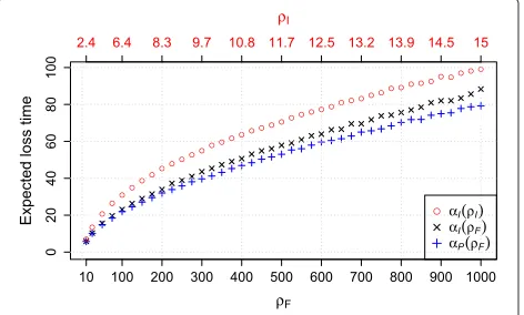
Loss time
The lineage loss time distributionfor a given ρ is the following distribution of times: Given an array in station-arity, when does the last spacer from the ancestral array gets lost? Theexpected lineage loss timeis the expectation of this distribution. Analogously, we define thepairwise loss time distributionas the distribution of times when two independently evolving lineages lost their last common spacer. In detail, we simulate two lineages starting from a common ancestor and track changes in both lineages simultaneously.tis the time when the deletion in one lin-eage results in the loss of all spacers that are present at that time in the other lineage. The pairwise loss time simulated is then 2tsince there were two lineages. The distribution is always approximated using 10,000 simulated pairs.
The expectations of these distributions is denoted by
αl(ρI)(expected lineage loss time under the independent loss model givenρI),αp(ρI)(expected pairwise loss time for the independent loss model givenρI), and analogously with subscript F for the fragment loss model. In case the underlying ρ is clear, the argument is omitted. The expected lineage and pairwise loss times are lower for the fragment loss model (Figure 5). In the estimation, we set
ˆ
τ = αp(ρ)ˆ for a pair without overlap. Note that this is an underestimate of the time between two arrays since the loss time is an estimate of the minimum, i.e., the first time when two arrays lost common spacers.
Simulation
[image:7.595.58.294.533.675.2]Simulation under each model is implemented in a python program. Input is a phylogeny with branch lengths,ρand the type of the model. An ancestor length is drawn at the root of the phylogeny from the stationary distribution of the length model. Spacers are labelled arbitrarily. Then the tree is traversed in preorder and the descendent of each branch given its ancestor and branch lengthtis simulated as follows.
Figure 5Expected loss times for both models.αl- expected
lineage loss time,αp- expected pairwise loss time.αl(ρI)=αp(ρI),
thus only one is displayed. Correspondingρs are in one column, i.e., they result in the same expected length. Each point represents 10,000 simulations.
Start with the ancestors,n= |s|, current timetc=0.
1. Determine the time until the next event of each type:
(a) Draw a waiting time until the next insertion event from an exponential distribution with
rateλ.
(b) Draw the waiting times until the next deletion for each spacer or fragment. (b1) If the independent loss model is simulated,
drawn exponential waiting times, each with
rateμ.
(b2) If the fragment loss model is simulated, draw
n(n+1)
2 exponential waiting times with rateμ,
one for each fragment.
2. Find the minimal timetminover all times generated
in step 1.
3. tc=tc+tmin.
4. Iftc>t, returns as the sequence at the descendent
node.
5. Else the event that corresponds totminis realized, the
other events are discarded. Iftmincorresponds to an
insertion, one spacer with a new name is inserted. In case of the unordered model, the spacer is inserted at a random position, in the other cases it is always
inserted in the beginning ofs. Iftmincorresponds to a
deletion, modifys by deleting the corresponding
fragment or spacer.
6. Continue at step 1 with the modifieds.
Phylogeny computation using CRISPR distances
The sum of the estimated times given two strains,τ, can be interpreted as the distance between these two strains. These distances can be used to compute a distance-based phylogeny using neighbor joining [32] as was presented by Huson and Steel [33]. For the non-reversible models, however, there is more information available, since there is an estimate for the distance of the last common ancestor to each of the two strains. We use a modified neighbor joining method to utilize this information and refer to it asrooted neighbor joining. We describe the algorithm with an example.
Input: Fork taxa, all k2 pairs with rooted time esti-mates, that is dx,y for the distance to taxonx from the ancestor of the pair(x,y).
Output:A rooted phylogenetic tree with timest.
Algorithm:
1. Compute the weights for all pairs(x,y):
wx,y=
z=x,y
(dx,z−dx,y+dy,z−dy,x)
=(2−k)(dx,y+dy,x)+
z=x,y
2. Choose the pair with maximal weightwx,y. Create a
new noder that is the ancestor of(x,y)with
tr,x =dx,yandtr,y=dy,x.
3. Compute the distances between all other nodesz and
r:
dr,z= 1
2(dx,z−dx,y+dy,z−dy,x),dz,r = 1
2(dz,x+dz,y)
4. If only one node is left, return it as the root, else continue with step 1.
By construction, the method results in the correct rooted tree if the distances were extracted from a rooted tree. We show this for three taxa.
For three taxa, there is only one clade, we choose (1,2) to be the correct clade. Then the branch lengths are given in Figure 6.
Iteration 1:
Distance matrixdx,y=
⎛ ⎝
1 2 3
1 0 a a+c
2 b 0 b+c
3 d d 0
⎞
⎠.
Weights:w1,2= −(d1,2+d2,1)+d1,3+d2,3= −(a+b)+ a+c+b+c= 2c,w1,3 = −(a+c+d)+a+d = −c, w2,3 = −(b+c+d)+b+d = −c. Thus for all possible a,b,c,d,w1,2 = argmaxi,jwi,jand the correct grouping is chosen by the algorithm.
Create node 4 witht4,1 = d1,2 = aandt4,2 = d2,1 = b.
The tree is now(t1:a,t2:b)4.
Iteration 2:
Distance matrixdx,y=
3 4
3 0 d
4 c 0
.
There is only one pair, create node 5 with t3,5 = d3,4 = d and t4,5 = d4,3 = c. The resulting tree is ((t1:a,t2:b)4:c,t3:d)5. Apart from the internal labels, this tree is identical to the original one (Figure 6).
We abbreviate the method rooted neighbor joining with times from the fragment loss model byRNJF, analogously forNJ and subscriptOfor the ordered model and sub-scriptUfor the unordered model.
Yersinia pestisdata set
We downloaded available Yersinia pestis genomes (final list in Table 2). Unfinished strains were included if open reading frames have been annotated. Cas genes are detected using HMMER [34] and the profiles defined previously for the Ypest type (ftp://ftp.ncbi.nih.gov/pub/ wolf/_suppl/CRISPRclass/crisprPro.html [5]). Unfinished strains were excluded if cas genes were detected on differ-ent contigs. In these cases, not all cas genes were available.
t1
t2
t3
d
c
[image:8.595.305.539.85.350.2]b
a
Figure 6Rooted tree of three taxa with branch lengths.
The whole locus was extracted, i.e., the sequence from the start ofcas1until the end ofcsy4. Nucleotide sequences from the resulting 19 strains were aligned using clustalw [35] into an alignment of 8555 sites that is subsequently used for phylogeny estimation with iqpnni [36].
Putative CRISPR arrays for the 19 strains are extracted using CRISPRfinder [37]. True CRISPR elements are found by comparing the repeat sequence to the known
Yersinia pestis repeat. The three types of CRISPR arrays are distinguished by their last degenerated repeat [8]. In total, four CRISPR arrays are missing from the CRISPRfinder results. In these cases, we located the respective leader in the genome and extracted repeats and spacers manually. These arrays harbor none or one spacer. For each data set, spacers were assigned the same identity if they show more than 90% sequence similarity. This is a natural cutoff to choose since there was no pair of spacers with similarity between 65% and 90%. Spacer sequences can be found in Additional file 2 for Yp1, in Additional file 3 for Yp2 and in Additional file 4 for Yp3.
Results
Parameter estimation for simulated pairs
Table 2 CRISPR arrays fromYersinia pestisgenomes
Strain Accession Yp1 Yp2 Yp3
91001 GenBank:NC_005810.1 21-1-0 3-2-1-0 0
a1122 GenBank:NC_017168.1 7-6-2-5-1-4-3-0 4-3-2-1-0 2-1-0
angola GenBank:NC_010159.1 8-1-4-0
antiqua GenBank:NC_008150.1 10-9-1-4-3-0 5-2-0 2-1-0
ca88-4125 GenBank:ABCD00000000.1 7-6-2-5-1-4-3-0 4-3-2-1-0 2-1-0
co92 GenBank:NC_003143.1 7-6-2-5-1-4-3-0 4-3-2-1-0 2-1-0
d106004 GenBank:NC_017154.1 6-2-5-1-4-3-0 3-2-1-0 2-1-0
d182038 GenBank:NC_017160.1 11-6-2-5-4-3-0 3-2-1-0 2-1-0
e1979001 GenBank:AAYV00000000.1 11-6-2-5-4-3-0 3-2-1-0 2-1-0
f1991016 GenBank:ABAT00000000.1 7-6-2-5-1-4-3-0 4-3-2-1-0 2-1-0
harbin35 GenBank:NC_017265.1 4-31-01 3-2-1-0 2-1-0
india195 GenBank:ACNR00000000.1 7-6-2-5 4-3-2-1-0 2-1-0
kim10 GenBank:NC_004088.1 4-3-0 31-2-1-0 2-1-0
mg05-1020 GenBank:AAYS00000000.1 7-6-2-5-1-4-3-0 4-3-2-1-0 2-1-0
nepal516 GenBank:NC_008149.1 02 3-2-1-0 2-1-0
pestoidesa GenBank:ACNT00000000.1 2-1-03 6-3-2-0 1-01
pestoidesf GenBank:NC_009381.1 12-5-1-4-3-0 9-8-6-1-7-0 4-3-2-1-0
pexu2 GenBank:ACNS00000000.1 7-6-2-5-1-4-3-0 4-3-2-1-0 2-1-0
z176003 GenBank:NC_014029.1 6-2-5-1-4-3-0 3-2-1-0 2-1-0
Spacers are grouped and assigned a unique number for each array if they show>90%sequence similarity. Different variants are marked by superscript and ignored in
the analysis. The leader-proximal end is displayed on the left. Spacer sequences can be found in Additional file 2 for Yp1, in Additional file 3 for Yp2 and in Additional file 4 for Yp3.
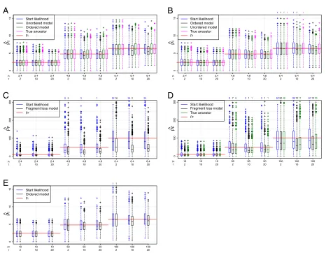
First, we compare the simulatedρ with its estimation.
ρis estimated based on the start likelihood using the sta-tionary distribution or on the full likelihood summing over all pairs. Note that the start likelihood functions are equal for both independent loss models. The estimates based on the start likelihood and on the full likelihood are very similar for the independent loss models (Figure 7A, B). For the fragment loss model,ρFtends to be underesti-mated for the full likelihood but not for the start likelihood (Figure 7D). The segmentation of ancestors and descen-dants into independent pairs may cause this bias. This segmentation ignores the probability of deletion events spanning multiple segments and can result in an overesti-mation ofμFand thus in an underestimation of the ratio
ρF=λ/μF.
We also compare the estimation using the full likelihood with the ancestor fixed to the true ancestor and using the full likelihood with summing over possible ancestors. The estimated values ofρ are very similar, which leads to the conclusion that the ancestor enumeration works appropriately.
Next, we use the same simulated data sets, but inves-tigate the results when using an incorrect model for the estimation. We only compare the models with single dele-tions among each other and the models with polarized
insertions among each other (see also Table 1). The inde-pendent loss models differ only in their insertions. When using the incorrect insertion model, ρˆI is very similar (Figure 7A, B). These models are also very similar in their construction. They are the same if after the first shared spacer there are no spacers unique to one strain. When using the incorrect deletion model, the correspondingρ tends to be estimated (Figure 7C, E). In detail, theρIthat is estimated under the ordered model from the data gen-erated under the fragment loss model is on average the
ρIcorresponding toρFused for the simulations (red line in Figure 7E). The underestimation ofρF is even present to a larger extent whenρF is estimated from data gener-ated under the ordered model compared to the estimation under the true model.
Times can only be estimated for pairs with overlap. The quality of the time’s estimation depends on the simulated
A
05
1
0
1
5
ρI
^
2.4 2.4 2.4 4.8 4.8 4.8 6.4 6.4 6.4
2 10 20 2 10 20 2 10 20
ρI τ
Start likelihood Unordered model Ordered model True ancestor ρI
B
0
5
10
15
ρI
^
2.4 2.4 2.4 4.8 4.8 4.8 6.4 6.4 6.4
2 10 20 2 10 20 2 10 20
ρI τ
1111 11 1
Start likelihood Ordered model Unordered model True ancestor ρI
C
0
1
00
200
300
ρF
^
2.4 2.4 2.4 4.8 4.8 4.8 6.4 6.4 6.4
2 10 20 2 10 20 2 10 20
ρI τ
95 3 1 5216 342 25
Start likelihood Fragment loss model ρF
D
0
1
00
200
300
ρF
^
10 10 10 50 50 50 100 100 100
2 10 20 2 10 20 2 10 20
ρF τ
876 311 211 625048 381011 401323
Start likelihood Fragment loss model True ancestor ρF
E
05
1
0
1
5
ρI
^
10 10 10 50 50 50 100 100 100
2 10 20 2 10 20 2 10 20
ρF τ
11
[image:10.595.60.536.89.451.2]Start likelihood Ordered model ρI
Figure 7Estimation ofρwith 2 arrays.(A) Simulations under the unordered model. (B,C) Simulations under the ordered model. (D,E) Simulations under the fragment loss model. A standard boxplot is shown. 1000 replicates are simulated under each setting. If present, the number of points outside the plot are listed above.
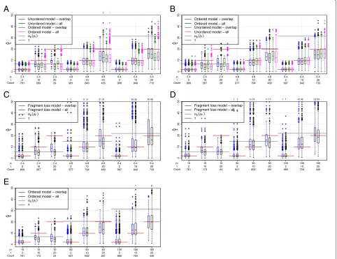
from the pairs with overlap only, decreases the average time estimated, if there are many empty pairs (Figure 8). This can be explained by two effects. First, the loss time is a minimum, i.e., the first time when two arrays lost common spacers. Second, shorter arrays occur more often among the pairs without overlap. That means,ρˆis smaller for these pairs and thus their loss time is smaller as well (Table 3).
Using the true model, we find that times are well esti-mated until a threshold depending on the simulatedρ. For example, for the independent loss model, for ρ = 4.8, only τ = 2 is well estimated, but for ρ = 6.4,τ = 2 andτ = 10 are well estimated. This threshold is below the expected pairwise loss time. Time estimation for the fragment loss model is more noisy and a slight overestima-tion can occur for intermediate times that may be related to the underestimation ofρfor these parameter settings (Figure 8D).
Time estimates for the incorrect independent loss model are very similar (Figure 8A, B). In general, the ordered model results in slightly lower time estimates. Small and intermediate times are overestimated when the ordered model is applied to data generated under the frag-ment loss model (Figure 8E), possibly because more events are necessary to explain this data. Applying the fragment loss model to ordered independent loss data also results in an overestimation for intermediate times (Figure 8C).
Parameter estimation for simulated phylogenies
Next we apply the estimation to data sets simulated on a phylogeny. The same values of ρas in the previous sim-ulations were used. Phylogenies of 10 taxa are generated under a Yule process and rescaled to a specific tree height (tree height of 1, 5, 10, 20 and 30, respectively).
A
0
1
02
03
04
0
5
0
τ
^
2.4 2.4 2.4 4.8 4.8 4.8 6.4 6.4 6.4
2 10 20 2 10 20 2 10 20
781 269 29 981 840 455 998 949 715
ρI τ Count
1 1
Unordered model − overlap Unordered model − all Ordered model − overlap Ordered model − all αp(ρI) τ
B
0
1
02
03
04
0
5
0
τ
^
2.4 2.4 2.4 4.8 4.8 4.8 6.4 6.4 6.4
2 10 20 2 10 20 2 10 20
809 267 26 977 794 460 997 942 733
ρI τ Count
Ordered model − overlap Ordered model − all Unordered model − overlap Unordered model − all αp(ρI)
τ
C
01
0
2
0
3
0
4
0
5
0
τ
^
2.4 2.4 2.4 4.8 4.8 4.8 6.4 6.4 6.4
2 10 20 2 10 20 2 10 20
809 267 26 977 794 460 997 942 733
ρI τ Count
11 99 3131 3535 9090 Fragment loss model − overlap
Fragment loss model − all αp(ρF)
τ
D
01
0
2
0
3
0
4
0
5
0
τ
^
10 10 10 50 50 50 100 100 100
2 10 20 2 10 20 2 10 20
761 173 24 921 602 261 965 704 440
ρF τ Count
11 1515 1111 11 4242 5253 Fragment loss model − overlap
Fragment loss model − all αp(ρF)
τ
E
01
0
2
0
3
0
4
0
5
0
τ
^
10 10 10 50 50 50 100 100 100
2 10 20 2 10 20 2 10 20
761 173 24 921 602 261 965 704 440
ρF τ Count
1 8
[image:11.595.59.541.88.459.2]Ordered model − overlap Ordered model − all αp(ρI) τ
Figure 8Estimation of times with 2 arrays.(A) Simulations under the unordered model. (B,C) Simulations under the ordered model. (D, E) Simulations under the fragment loss model.τis the sum of the times from the ancestor to both descendants. Only pairs with overlap are included for “overlap”, the number of pairs is given by “Count”. A standard boxplot is shown. 1000 replicates are simulated under each setting. If present, the number of points outside the plot are listed above.
variance. The variance in the estimates is higher for the fragment loss model compared to the independent loss models. For the independent loss model, the mean of the
ˆ
ρ-values is usually close toρ (Figure 9). Under the frag-ment loss model,ρfor the intermediate times are underes-timated (Figure 9D). Times are again well esunderes-timated until a threshold depending on the simulated ρ (Figure 10). For the fragment loss model, times are overestimated for intermediate tree heights (Figure 10D).
Yersinia pestisanalysis
Yersinia pestis genomes generally harbor three CRISPR
arrays types, called Yp1, Yp2, and Yp3. All three array types have the same repeat sequence and only one set of cas genes of the Ypest type is present in the genome. We demonstrate the methods using threeYersinia pestis
data sets (Table 4). One data set was assembled from
19 sequenced genomes (see Materials and Methods and Table 2). Pourcel et al. [8] investigate 62 strains but Yp1 is only present in 60 of them. They sequence Yp2 in 15 of them but give no detailed information about Yp3, thus it was not included. Cui et al. [27] investigate 131 strains, including published genomes andYersinia pestis isolates from Asia. The three arrays are present in all of them but sequence information for Yp2 and Yp3 is missing in 6 and 5 strains, respectively.
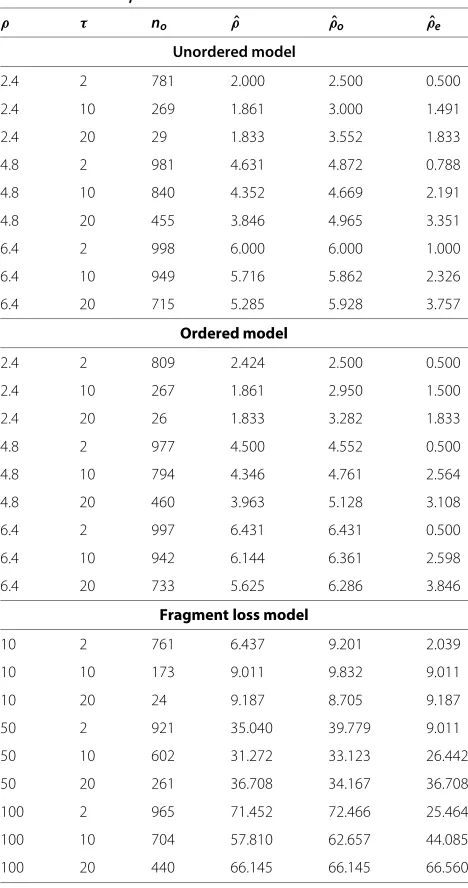
Table 3 Medianρestimates
ρ τ no ρˆ ρˆo ρˆe
Unordered model
2.4 2 781 2.000 2.500 0.500
2.4 10 269 1.861 3.000 1.491
2.4 20 29 1.833 3.552 1.833
4.8 2 981 4.631 4.872 0.788
4.8 10 840 4.352 4.669 2.191
4.8 20 455 3.846 4.965 3.351
6.4 2 998 6.000 6.000 1.000
6.4 10 949 5.716 5.862 2.326
6.4 20 715 5.285 5.928 3.757
Ordered model
2.4 2 809 2.424 2.500 0.500
2.4 10 267 1.861 2.950 1.500
2.4 20 26 1.833 3.282 1.833
4.8 2 977 4.500 4.552 0.500
4.8 10 794 4.346 4.761 2.564
4.8 20 460 3.963 5.128 3.108
6.4 2 997 6.431 6.431 0.500
6.4 10 942 6.144 6.361 2.598
6.4 20 733 5.625 6.286 3.846
Fragment loss model
10 2 761 6.437 9.201 2.039
10 10 173 9.011 9.832 9.011
10 20 24 9.187 8.705 9.187
50 2 921 35.040 39.779 9.011
50 10 602 31.272 33.123 26.442
50 20 261 36.708 34.167 36.708
100 2 965 71.452 72.466 25.464
100 10 704 57.810 62.657 44.085
100 20 440 66.145 66.145 66.560
Estimation with two arrays under the correct model, same data as Figures 7 and
88.no- number of pairs with overlap,ρˆo- median ofρestimates of pairs with
overlap only,ρˆe- median ofρestimates of pairs without overlap only.
time between the arrays divided by the pairwise loss time, where maximum diversity is 1. Yp3 has the lowest diver-sity for each data set it is present. However, the results for the other array types differ. Pourcel et al. [8] argued that Yp1 is the most dynamic CRISPR locus. Based on the data of Pourcel et al. (data set 2), diversity is similar in Yp1 and Yp2 under the independent loss model, and diversity is lower in Yp1 than in Yp2 under the fragment loss model. This discrepancy is resolved when comparing the average times. The average time is larger in Yp1 than in Yp2 for each model. Thus there are more events present in Yp1 compared to Yp2. When considering that the longer arrays
in Yp1 could resolve larger times, the diversity results in a similar value. Data set 3 [27] shows higher diversity in Yp1 compared to Yp2 under all three models. Diversity in Yp1 is also higher in data set 3 compared to data set 2. Data set 3 thus captures a larger fraction of the diversity in CRISPR spacer content present inYersinia pestis.
Cas sequence data is only present for data set 1. The respective cas phylogeny contains few substitutions (Figure 11). The spacer distances are also displayed in a tree structure using the unrooted and rooted neighbor joining method (Figure 12). These trees contain substan-tially more changes than the cas gene phylogeny and there are also few incongruencies. The group (nepal516, harbin35) present in the cas phylogeny is not present in any CRISPR tree, but is compatible with the trees from Yp2 and Yp3. The group (pestoidesa, pestoidesf, angola) is contradicted in all trees. The rooted method tends to con-nect strains with few spacers directly to the root, for Yp1 this is nepal516 (having only one spacer) and for Yp2 and Yp3 this is angola (having an empty array). Note that the angola strain was indeed described to be a deep-rooting
Yersinia pestis strain [38]. For the slowly evolving locus Yp3, the clusters displayed by NJU andRNJF are equal, only the branch lengths differ and the clusters display the relationships well. In detail, there is a cluster for all strains having spacer 0, for all strains having spacer 1, and for all strains having spacer 2. The terminal branch leading to angola is much longer for NJU, since multiple deletions are needed that can be explained by only one event under the fragment loss model. On the other hand, the branches leading to pestoidesf have about the same length since there are only two observed insertions. For the other more diverse loci, trees display which strains are more divergent and which ones are more similar. For example,RNJF for Yp2 shows that angola, pestoidesf, antiqua and pestoidesa are more divergent, whereas the other strains are more similar to each other. Indeed, to convert between two of the other strains at most one event is needed, wheres to convert one of the four strains mentioned into any other one at least two events are necessary.
Discussion
A
0
5
10
15
ρI
^
2.4 2.4 2.4 2.4 2.4 4.8 4.8 4.8 4.8 4.8 6.4 6.4 6.4 6.4 6.4 1 5 10 20 30 1 5 10 20 30 1 5 10 20 30 ρI
Treeheight
1
11
Start likelihood Unordered model Ordered model ρI
B
05
1
0
1
5
ρI
^
2.4 2.4 2.4 2.4 2.4 4.8 4.8 4.8 4.8 4.8 6.4 6.4 6.4 6.4 6.4 1 5 10 20 30 1 5 10 20 30 1 5 10 20 30 ρI
Treeheight
Start likelihood Ordered model Unordered model ρI
C
05
0
1
0
0
150
200
250
300
ρF
^
2.4 2.4 2.4 2.4 2.4 4.8 4.8 4.8 4.8 4.8 6.4 6.4 6.4 6.4 6.4 1 5 10 20 30 1 5 10 20 30 1 5 10 20 30 ρI
Treeheight
1 5
4
4 4 27 12 2 1
Start likelihood Fragment loss model ρF
D
0
5
0
1
00
150
200
250
300
ρF
^
10 10 10 10 10 50 50 50 50 50 100 100 100 100 100 1 5 10 20 30 1 5 10 20 30 1 5 10 20 30 ρF
T reeheight
3
1 6 0 1
4 0 4 1 1 1
Start likelihood Fragment loss model ρF
E
0
5
10
15
ρI
^
10 10 10 10 10 50 50 50 50 50 100 100 100 100 100 1 5 10 20 30 1 5 10 20 30 1 5 10 20 30 ρF
Treeheight
[image:13.595.58.542.88.443.2]Start likelihood Ordered model ρI
Figure 9Estimation ofρwith 10 arrays.(A) Simulations under the unordered model. (B,C) Simulations under the ordered model. (D, E) Simulations under the fragment loss model. Data was simulated on random Yule trees rescaled to a specific treeheight. A standard boxplot is shown. 1000 replicates are simulated under each setting. If present, the number of points outside the plot are listed above.
these environments. Different CRISPR array types might show different dynamics and thus have different utility for strain typing. An observed switch in spacer dynamics on a phylogeny might suggest a change in CRISPR cost or environment.
The three models presented here capture different mechanisms of CRISPR evolution, namely polarized addi-tion of spacers and deleaddi-tion of multiple successive spacers (Table 1). The CRISPR spacer arrays used for the analysis are assumed to be homologous. CRISPR homology can be determined by synteny in genomic positions and by repeat and leader similarities.
Models are necessarily a simplification of the past biological process. In our model, we ignore population dynamics. Our insertion and deletion rates are, as the substitution rates in phylogenetics, a compound param-eter including the process of random changes and selec-tion. The model is based on a time-homogenous Markov
process and the dynamics are assumed to be in station-arity. Since an analysis is based on one species and one CRISPR type, it is reasonable to assume that the mech-anistic insertion and deletion rates are homogeneous across the set of strains analyzed. We can not exclude, however, that subsets of strains experienced a different environment and thus different selection pressure on their spacer content. Simulations showed that the number of spacers in an array is determined mainly by internal parameters, like spacer insertion rate and cost of having spacers, not by external parameters, like the number of viruses in an environment [15].
A
01
0
20
30
40
50
60
τ
^
2.4 2.4 2.4 2.4 2.4 4.8 4.8 4.8 4.8 4.8 6.4 6.4 6.4 6.4 6.4 1 5 10 20 30 1 5 10 20 30 1 5 10 20 30 ρI
Treeheight τ
Unordered model Ordered model αP(ρI)
B
0
10
20
30
40
50
60
τ
^
2.4 2.4 2.4 2.4 2.4 4.8 4.8 4.8 4.8 4.8 6.4 6.4 6.4 6.4 6.4 1 5 10 20 30 1 5 10 20 30 1 5 10 20 30 ρI
Treeheight τ Ordered model Unordered model αP(ρI)
C
01
0
20
30
40
50
60
τ
^
2.4 2.4 2.4 2.4 2.4 4.8 4.8 4.8 4.8 4.8 6.4 6.4 6.4 6.4 6.4 1 5 10 20 30 1 5 10 20 30 1 5 10 20 30 ρF
Treeheight
3 2 τ
Fragment loss model αP(ρF)
D
0
10
20
30
40
50
60
τ
^
10 10 10 10 10 50 50 50 50 50 100 100 100 100 100 1 5 10 20 30 1 5 10 20 30 1 5 10 20 30 ρF
Treeheight
1 τ
Fragment loss model αP(ρF)
E
01
0
20
30
40
50
60
τ
^
10 10 10 10 10 50 50 50 50 50 100 100 100 100 100 1 5 10 20 30 1 5 10 20 30 1 5 10 20 30 ρI
[image:14.595.57.541.86.461.2]Treeheight τ Ordered model αP(ρI)
Figure 10Estimation of times with 10 arrays.(A) Simulations under the unordered model. (B,C) Simulations under the ordered model. (D, E) Simulations under the fragment loss model. A standard boxplot is shown. 1000 replicates are simulated under each setting. If present, the number of points outside the plot are listed above.
In the context of birth and death processes it is known as the simple death-and-immigration process (e.g., [40]).
The times estimated under these models also allow a comparison to substitution rates if sequence data is avail-able. This analysis is however complicated by several facts. First, microbial genomes often harbor multiple CRISPR arrays. As a consequence, it is not clear how to combine these estimates to make a comparison possible. Second, spacer content might be different for very closely related strains. Then only a few polymorphisms are available and the substitution rate cannot be estimated reliably. Finally, frequent horizontal gene transfer of the CRISPR/Cas sys-tem has been suggested (e.g., [41]), and thus CRISPR rates can only be compared to substitution rates of cas genes.
The parameter estimation as presented here does not use an explicit phylogeny. This is advantageous since no search through tree space is necessary or no pre-computed phylogeny needs to be given. The latter may
Table 4Yersinia pestisdata sets
Data set Array Strains Avg. length Avg. overlap
Yp1 19 5.737 0.658
1 (Table 2) Yp2 19 4.211 0.741
Yp3 19 2.789 0.865
2 [8] Yp1 60 6.8 0.905
Yp2 15 4.733 0.847
Yp1 131 6.542 0.588
3 [27] Yp2 125 4.584 0.814
Yp3 126 2.99 0.931
[image:14.595.304.540.578.706.2]Table 5Yersinia pestisresults
Unordered model Ordered model Fragment loss model
Data Avg. Avg. Avg. Avg. Avg. Avg.
set Array ρˆI time diversity ρˆI time diversity ρˆF time diversity
Yp1 5.555 5.802 0.2271 5.527 5.947 0.2362 46.24 4.96 0.3331
1 Yp2 4.027 3.479 0.2188 4.005 3.538 0.2241 22.87 3.645 0.3108
Yp3 2.667 1.506 0.1755 2.667 1.486 0.1772 11.36 1.313 0.2061
2 Yp1 6.625 4.726 0.1445 6.624 4.761 0.1446 90.21 3.859 0.188
Yp2 4.676 2.984 0.1494 4.655 3.082 0.156 28.61 3.701 0.2748
Yp1 6.401 9.138 0.2943 6.36 9.259 0.2983 80.76 9.741 0.4408
3 Yp2 4.613 3.329 0.1707 4.607 3.379 0.1749 39.31 3.359 0.2492
Yp3 2.969 0.7221 0.07339 2.959 0.7184 0.07114 12.6 0.8776 0.1025
not be possible since no external information might resolve the CRISPR relationships. On the other hand, only a distance-based approach is available to display the CRISPR relationships. We can use the rooted dis-tance from non-reversible models to compute rooted non-clocklike distance-based trees.
We find that estimation of the rate parameter performs well on average, but the estimates under the indepen-dent loss models show a lower variance. The fragment loss model tends to an underestimation and may be affected by the factorization of the likelihood function. The time estimates are most accurate for shorter times. For longer times, the absence of overlap complicates an accurate time estimation. In the analyses presented here, the different models result in similar estimates. If the incorrect loss model is applied, the correspondingρtends to be estimated fairly accurately. There is also no clear bias that affects the time estimation under an incorrect model. Note that there is a wide range of possible models accounting for fragment deletions. We chose one with the
same instantaneous rate for each possible fragment, i.e., ignoring fragment length. This simplification is mainly for computational reasons. Future work on other fragment loss models, including lengths of fragments, might lead to a better fit for CRISPR spacer data.
We compare the estimations between data sets and between different CRISPR arrays present in a genome. Three Yersinia pestis data sets were chosen since they harbor three CRISPR array types and thus this data sets allows for comparison between data sets and between CRISPR array types evolving with different dynamics. Using this data set, we findρestimates to be similar using two published data sets but lower in a data set assembled from published genomes. Time and diversity estimates differ between data sets thus the presented methods allow comparisons of the diversity of CRISPR loci sampled from different populations.
For theYersinia pestisdata from published genomes, we observe only few differences in the cas gene sequences but a high diversity at the spacer level. Thus substitution
angola
1.0E-4
d106004
antiqua
pestoidesf pexu2
india195
mg05-1020
ki m 10
nepal516
harbin35
co9 2
z176003
91001
f1991016
e1979001
pestoidesa
d182038
ca88-4125 a112
2
[image:15.595.56.539.517.716.2]A
2 .0 kim 10 harbin3 5 pexu2 d10600 4 india19 5 ca88-412 5 mg05-102 0 a1122 nepal51 6 91001 co92 f1991016 d1820 3 8 pestoidesa pest oide sf z1760 03 e197900 1 angola antiqu aB
2 .0 f199101
6 co92 mg05-102 0 harbin 35 pestoides f a1122 nepal51 6 pest oide sa angola ant iqua 9100 1 d182038 d10600 4 e197900 1 z17600 3 c a88-41 25 india19 5 pexu2 kim 1 0
C
2 .0 india19
5 f199101 6 angola z1760 03 d10600 4 kim1 0 pestoidesf antiq ua e197900 1 9 1001 pest oides a a11 22 nepal5 16 co92 ca88-412 5 mg05-102 0 harbin3 5 pe xu2 d18203 8
D
2 .0 ant iqua pestoide sf 9100 1 pexu2 kim10 z1760 03 pest oide sa mg05-10 2 0 a112 2 e19790 01 f199101 6 nepal51 6 d1820 38 india19 5 angola co92 ca88-4125 d10600 4 harbin 35E
2 .0 india19 5 pes toides f e19790 01 ca88-412 5 pexu2 z17600 3 9 1 0 0 1 [image:16.595.57.539.85.680.2]nepal5 16 co92 angola pestoidesa f1991016 antiqu a d18203 8 kim10 harbin3 5 mg05-102 0 d10600 4 a112 2
F
2 .0 antiqua ca88-412 5 co92 9100 1 pexu2 d10600 4 harbin3 5 d18203 8 angola pes toides f kim 10 a1122 pestoides a e197900 1 z17600 3 india1 95 mg05-102 0 nepal51 6 f199101 6Figure 12Trees using the CRISPR spacer data from data set 1.(A,C,E)NJU: Neighbor joining tree of times from the unordered model. (B,D,F)RNJF: Rooted neighbor joining tree of times from the fragment loss model.(A,B)Yp1,(C,D)Yp2,(E,F)Yp3. Branch lengths correspond to
rates cannot be compared with reliability, but nucleotide and CRISPR spacer data provide phylogenetic informa-tion at very different time scales. It is possible to compute cas gene phylogenies on the species level (e.g., [41]). In contrast, spacer information could be utilized for closely related strains that have only few differences in the other nucleotide sequences, which has already been done in using CRISPR in strain typing (e.g., [8,10,11]). The method presented here can be used to define groups based on the clustering or to find relationships between groups.
A steadily growing literature suggests many other pos-sible mechanisms of CRISPR evolution apart from polar-ized addition and fragment deletion. Spacer insertion can happen together with an internal deletion [42], or at an internal repeat [43]. Spacers or whole fragments may be duplicated [44]. And present spacers can guide the acqui-sition of new spacers from the same DNA molecule [45]. Note that these results affect only the insertion step of the CRISPR evolution process. But the fragment deletion model as it is presented here is based on the polarized insertion assumption. Combining an unordered insertion with a fragment deletion process is currently infeasible. Given these studies and the fact that the models pre-sented here do not give substantially different results, the unordered model may be a robust choice for estimating rate and time parameters from CRISPR array data. Note that several simplifications are possible for the likelihood computation under this model. First, for the start likeli-hood, the estimate of the Poisson parameter is well known to be the mean of the data values. Second, it is reversible, thus only the time between two arrays can be estimated and the ancestor generation can be omitted. Third, the loss time can be calculated analytically and does not need to be acquired using simulations. To make the model com-parisons fair, the same computational approach is used for all models in this paper. But it is possible to implement a more efficient approach for the unordered model. Under this model, an algorithm for the likelihood computation on a phylogeny is also potentially feasible.
Conclusions
We present different models specific for CRISPR spacer content evolution. The three models differ in two aspects. First, fragment loss models differ from the independent loss models since they allow the loss of a succession of spacers in one event. Second, the unordered indepen-dent loss model differs from the others since spacers can be incorporated throughout the array, not only on one end. A probabilistic model for each of these three mod-els is presented here. We developed an approach derived from a well behaved stationary distribution, to establish the bounds on the state space that is a priori infinite. We find that the simpler model, without fragment dele-tions, is more robust. Distance-based phylogenies can be
calculated from the time estimates, but the rapid change of spacer content restricts this method to closely related strains with similar spacer content.
In summary, the models facilitate quantitative state-ments about the spacer dynamics of microbial communi-ties. Thus comparisons are possible, for example, between strain collections from one species at different locations or between different homologous CRISPR arrays in the same set of species.
Additional files
Additional file 1: Proof of equation (3).
Additional file 2:Yersinia pestisspacer sequences for data set 1 Yp1 in fasta format.
Additional file 3:Yersinia pestisspacer sequences for data set 1 Yp2 in fasta format.
Additional file 4:Yersinia pestisspacer sequences for data set 1 Yp3 in fasta format.
Competing interests
Both authors declare that they have no competing interests.
Authors’ contributions
JPB and AK designed the project. AK implemented the methods, carried out simulations and estimations and wrote the manuscript. Both authors discussed the results and the manuscript. Both authors read and approved the final manuscript.
Acknowledgements
The authors would like to thank Christoph Lampert, Sebastian Matuszewski and Rodrigo A.F. Redondo for productive discussions and helpful comments on the manuscript, and two anonymous reviewers for valuable comments improving the manuscript.
Received: 22 November 2012 Accepted: 14 February 2013 Published: 26 February 2013
References
1. Barrangou R, Fremaux C, Deveau H, Richards M, Boyaval P, Moineau S, Romero DA, Horvath P:CRISPR provides acquired resistance against viruses in prokaryotes.Science2007,315(5819):1709–1712. 2. Marraffini LA, Sontheimer EJ:CRISPR interference limits horizontal
gene transfer in staphylococci by targeting DNA.Science2008,
322:1843–1845.
3. Bolotin A, Quinquis B, Sorokin A, Ehrlich SD:Clustered regularly interspaced short palindrome repeats (CRISPRs) have spacers of extrachromosomal origin.Microbiology2005,151(Pt8):2551–2561. 4. Wiedenheft B, Sternberg SH, Doudna Ja:RNA-guided genetic silencing
systems in bacteria and archaea.Nature2012,482(7385):331–338. 5. Makarova KS, Aravind L, Wolf YI, Koonin EV:Unification of Cas protein
families and a simple scenario for the origin and evolution of CRISPR-Cas systems.Biol Direct2011,6:38.
6. Tyson GW, Banfield JF:Rapidly evolving CRISPRs implicated in acquired resistance of microorganisms to viruses.Environ Microbiol
2008,10:200–207.
7. Horvath P, Romero Da, Coûté-Monvoisin AC, Richards M, Deveau H, Moineau S, Boyaval P, Fremaux C, Barrangou R:Diversity, activity, and evolution of CRISPR loci in streptococcus thermophilus.J Bacteriol
2008,190(4):1401–1412.
8. Pourcel C, Salvignol G, Vergnaud G:CRISPR elements in yersinia pestis acquire new repeats by preferential uptake of bacteriophage DNA, and provide additional tools for evolutionary studies.Microbiology
2005,151(Pt 3):653–163.