Scalable Automation of Online Network Attack Characterization

Theses Thesis/Dissertation Collections

7-2014

Scalable Automation of Online Network Attack

Characterization

Ryan T. Rawlins

Follow this and additional works at:http://scholarworks.rit.edu/theses

This Thesis is brought to you for free and open access by the Thesis/Dissertation Collections at RIT Scholar Works. It has been accepted for inclusion in Theses by an authorized administrator of RIT Scholar Works. For more information, please [email protected].

Recommended Citation

Characterization

by

Ryan T. Rawlins

A Thesis Submitted in Partial Fulfillment of the Requirements for the Degree of Master of Science

in Computer Engineering

Supervised by

Associate Professor and Department Head Dr. Shanchieh Jay Yang Department of Computer Engineering

Kate Gleason College of Engineering Rochester Institute of Technology

Rochester, New York July 2014

Approved by:

Dr. Shanchieh Jay Yang, Associate Professor and Department Head

Thesis Advisor, Department of Computer Engineering

Dr. Andres Kwasinski, Associate Professor

Committee Member, Department of Computer Engineering

Dr. Raymond Ptucha, Assistant Professor

Rochester Institute of Technology Kate Gleason College of Engineering

Title:

Scalable Automation of Online Network Attack Characterization

I, Ryan T. Rawlins, hereby grant permission to the Wallace Memorial Library to repro-duce my thesis in whole or part.

Ryan T. Rawlins

Acknowledgments

I would like to thank my thesis advisor and committee members for their guidance and time throughout the research process. I would also like to thank my friends and family for

Abstract

Scalable Automation of Online Network Attack Characterization

Ryan T. Rawlins

Supervising Professor: Dr. Shanchieh Jay Yang

Cyber attacks to enterprise networks and critical infrastructures are becoming more preva-lent and diverse. Timely recognition of attack strategies and behaviors will assist analysts or resilient network defense systems in deploying effective means in anticipation of fu-ture threats. An attack can be characterized by the sequences of observed events that are relevant to critical assets. Earlier work has developed a semi-supervised learning frame-work to process large-scale events and extract attack behaviors. While the frameframe-work is designed to support online processing, the implementation requires extension and restruc-turing to support scalable automation of sustainable online network attack characterization.

Acknowledgments iii

Abstract iv

1 Introduction 1

1.1 Background . . . 1

1.2 Motivation . . . 2

2 Related Work 4 2.1 Attack Segmentation and Model Generation . . . 4

2.2 Attack Characterization . . . 5

2.2.1 Anomaly-Based Detection with Statistical Analysis . . . 6

2.2.2 Time Zones . . . 7

2.2.3 Flow Detection of P2P Botnets . . . 8

2.3 Intrusion Detection System Alert Correlation . . . 9

2.4 Capture the Flag Data . . . 11

3 Methodology 13 3.1 Functionality Updates . . . 14

3.1.1 MySQL Databases . . . 14

3.1.2 Feature and Graph Plots . . . 16

3.1.3 Environment Changes . . . 17

3.2 Algorithmic Changes . . . 19

3.2.1 New Observables . . . 19

3.2.2 New Features . . . 22

3.2.2.1 Absolute Time . . . 24

3.2.2.2 Time Intensity . . . 26

3.2.2.3 Alert Entropy . . . 28

3.2.3 Revision of the Model Introduction Strategy . . . 30

3.2.4 Revision to the Expectation Maximization (EM) Phase . . . 34

3.2.5 Implementation of Data Collection Metrics . . . 34

4 Results 36 4.1 Design of Experiments . . . 36

4.2 Feature Evaluation . . . 37

4.2.1 Determining a Baseline Measurement . . . 38

4.2.2 Performance of Feature Groups with CAIDA Data . . . 44

4.2.3 Performance of Feature Groups with iCTF2008 Data . . . 53

4.3 Behavior Interpretation . . . 61

5 Conclusions 69 5.1 Future Work . . . 70

3.1 Previously Implemented Features [20] . . . 23

3.2 Newly Implemented Features . . . 24

4.1 Feature Subgroups to Characterize Traffic . . . 37

4.2 Sample of Feature Distributions for Empirical Model 1 . . . 58

4.3 Sample of Feature Distributions for Empirical Model 3 . . . 58

4.4 Comparison of ASGs Generated from “New” and “Original” Feature Sets . . 59

4.5 Comparison of Confidence Data from “New” and “Original” Feature Sets . . 60

3.1 Overview of Algorithm and Revisions . . . 13

3.2 MySQL Connections Closed After Exception . . . 14

3.3 Example of Node to be Removed . . . 15

3.4 Feature Display Tab Not Showing Information . . . 16

3.5 Feature Display Tab Fixed . . . 17

3.6 Example Parallel Coordinate Plot . . . 18

3.7 Example of Snort Alert File . . . 19

3.8 Example of Bro Log . . . 20

3.9 Bro Log Processed into a CSV File . . . 21

3.10 Snort Alerts Processed into a CSV File . . . 21

3.11 Overview of Processing Flow . . . 21

3.12 Example of Deterministic Alert Behavior . . . 29

3.13 Example of Stochastic Alert Behavior . . . 29

3.14 Example of ASG Before Model Introduction Revisions . . . 33

3.15 Example of ASG After Model Introduction Revisions . . . 33

4.1 Baseline Model from CAIDA Data . . . 39

4.2 Na¨ıve Model from CAIDA Data . . . 39

4.3 Models Generated by Relevant Group for CAIDA Data . . . 40

4.4 Confidence Data of Relevant Group for CAIDA Data . . . 41

4.5 Parallel Coordinate Plot for Empirical Model 0 Feature Space . . . 42

4.6 Parallel Coordinate Plot for Empirical Model 3 Feature Space . . . 42

4.7 Parallel Coordinate Plot for Empirical Model 4 Feature Space . . . 43

4.8 Parallel Coordinate Plot for Empirical Model 12 Feature Space . . . 43

4.9 ASG Generated from Temporal Features on CAIDA Data . . . 44

4.10 Empirical 0 Model of Temporal Features on CAIDA Data . . . 45

4.11 Empirical 1 Model of Temporal Features on CAIDA Data . . . 45

4.12 Confidence Measurement of Temporal Features on CAIDA Data . . . 46

4.13 ASG of Original Features on CAIDA Data . . . 47

4.14 Confidence Measurement of Original Features on CAIDA Data . . . 47

4.15 Empirical Model 0 of Original Features on CAIDA Data . . . 48

4.16 Empirical Model 1 of Original Features on CAIDA Data . . . 49

4.17 Empirical Model 3 of Original Features on CAIDA Data . . . 49

4.18 ASG of Critical Features on CAIDA Data . . . 50

4.19 Confidence of Critical Features on CAIDA Data . . . 51

4.20 Empirical Model 0 of Critical Features on CAIDA Data . . . 52

4.21 Empirical Model 11 of Critical Features on CAIDA Data . . . 52

4.22 ASG of Relevant Features on iCTF2008 Data . . . 53

4.23 Na¨ıve ASG from iCTF2008 Data . . . 53

4.24 Confidence Data of Relevant Features on iCTF2008 Data . . . 54

4.25 Empirical Model 0 of Relevant Features on iCTF2008 Data . . . 55

4.26 ASG of Critical Features on iCTF2008 Data . . . 55

4.27 Confidence Data of Critical Features on iCTF2008 Data . . . 56

4.28 Empirical Model 1 of Critical Features on iCTF2008 Data . . . 57

4.29 Empirical Model 3 of Critical Features on iCTF2008 Data . . . 57

4.30 Network Topology for iCTF2008 Game . . . 61

4.31 Full ASG with Scanning and Island Hopping . . . 63

4.32 Network Topology Scan iCTF2008 . . . 64

4.33 Island Hop Example . . . 65

4.34 Second Stage Island Hop Example . . . 66

4.35 iCTF2008 Empirical 0 Model Feature Space . . . 67

4.36 iCTF2008 Empirical 1 Model Feature Space . . . 68

3.1 Euclidean Distance . . . 25

3.2 Dynamic Time Warp . . . 25

3.3 Absolute Distance in Time . . . 25

3.4 Probability of an Absolute Time . . . 26

3.5 Alternate Probability of an Absolute Time . . . 26

3.6 Packet Rate of an Edge . . . 27

3.7 Probability of an Edge Rate . . . 28

3.8 Probability of an Alert Value . . . 30

3.9 Reduced Equation for Probability of an Alert Value . . . 30

3.10 Model Graph Efficiency . . . 31

3.11 Graphical Prior Probability . . . 32

3.12 Revised Model Introduction Equation . . . 32

3.13 Average Value . . . 35

3.14 Standard Deviation . . . 35

3.15 Standard Error . . . 35

Chapter 1

Introduction

1.1

Background

The ability to identify and characterize cyber attacks helps to provide more efficient and appropriate defenses. This capability provides the backbone for prompt and effective identification of attacks from malware designed by users with malicious intents. An attack can be characterized by the sequences of observed events that are relevant to critical assets. Examples of attack types include worms, viruses and botnets. A worm is a standalone com-puter program that maliciously exploits security vulnerabilities in a target machine to gain access to a network and spread to new targets. Computer viruses look to replicate them-selves and infect other programs to either steal information, occupy bandwidth or corrupt data. A botnet is a collection of computers known as bots that are under the control of a remote user known as a botmaster. This collection of machines is then used in coordinated cyber attacks, such as distributed denial of service (DDoS), without the knowledge or per-mission of the owners of each compromised machine. Unique characteristics describe each type of attack which can be used to identify when one is encroaching upon a network.

sense that it can accommodate a work load that varies in size.

A semi-supervised machine learning based framework developed by [20] processes large-scale events and extracts attack behaviors. Bayes’s Theorem is utilized to calculate posterior probabilities to determine if an actor is likely to be part of a malicious behavior resolved from packet level features. An actor is an entity like a bot or hacker who acts in a malicious manner. Before incoming traffic can be analyzed for specific traits related to each behavior, it has to be processed in a couple of phases. First, a target of interest within the network topology is chosen so incoming traffic can be related to it. Next, the traffic relevant to the resource being attacked must be separated from other potentially unrelated traffic. Following this, the different behaviors that exist within this sub-set of the capture must be identified for classification. This final step can be difficult to isolate due to the extensive amount of variation in the possible behaviors that can be observed from a cyber attack, such as backscatter. Backscatter occurs when a machine is the target of a DDoS attack utilizing multiple spoofed IP addresses. The machine will not be able to distinguish between legitimate traffic and spoofed traffic from a malicious source. Responses sent from the target machine will go to each spoofed address, provided by the malicious source, gen-erating a lot of background noise.

While the framework in [20] was designed to support online processing, the implemen-tation required extension and restructuring. Packets were the only supported source of data which limited the accuracy and functionality of the application. Support was added to al-low metadata to be incorporated as a source of input utilizing the alert strings. Additional features, in conjunction with alternative sources of input data, help to better define behav-iors.

In this scenario, training the framework to properly define the behaviors of collaborat-ing actors is difficult as data is received in an unsupervised fashion. Unsupervised learncollaborat-ing systems do not have a ground truth associated with the training data so it is difficult to know for sure if data is being properly grouped. Typically, this is related to a clustering problem where groups are automatically generated from a dataset. To model the traffic flow on a typical network, the framework was configured with online learning. Online learning looks at one data point at a time to update the feature distributions of its models. The frame-work uses online unsupervised techniques to classify packets observed from the netframe-work. This creates a hybrid problem in trying to both efficiently cluster the data while properly classifying new samples. Each new sample will change the distributions that represent the models in the system which, in turn, effects how well this sample and those before it fit into these models.

1.2

Motivation

of the tools necessary to secure and maintain a network, it is difficult for a security analyst to maintain situational awareness of any one resource at any given time. The work done by [20] remedies this by providing a software tool and framework that provides situational awareness to a target of interest provided by the user.

This framework contained some limitations that prevented an analyst, or other tools, from fully utilizing the information generated. Originally, the main source of data was re-stricted to packet capture data stored in either a MySQL database or a log file. Existing tools such as Network Intrusion Detection Systems (NIDS) provide metadata that describe the traffic they observe. Incorporating multiple sources of data into one tool helps to bridge the gap between all of these utilities.

System administrators and security analysts will be able to view a larger amount of information in one consolidated application. This will also help to facilitate better commu-nication between analysts and those developing the tools that they use. The analysts will be able to look at the data that matters the most to them when determining when an attack has occurred. Developers can correlate this data to techniques that help collect and display this information in a more efficient manner.

Chapter 2

Related Work

To ensure a more robust and scalable environment for network attack characterization, it is necessary to first understand the inner workings of the original framework. Since the framework relies on a na¨ıve Bayesian classifier within an online, unsupervised machine learning environment, different features are required so each new input can be classified correctly. Most of the available packet level features had been previously implemented, with a high success rate, so new observables were sought out. These new features were needed to test the hypothesis that expanding the dimensionality of the input data would provide more precise clustering of the attack behaviors. In an unsupervised machine learn-ing configuration, there is no labeled dataset to check against durlearn-ing development. This creates the need for alternative methods to evaluate the performance of the features utilized in the clustering process.

2.1

Attack Segmentation and Model Generation

Strapp [20] worked to create an extensive framework, implemented in a software tool, that reads in packet level data and provides a higher level view of actors, who may be collaborating together to attack a network. This provides situational awareness around a given target of interest in a network allowing an analyst to examine events related to the given resource. The target of interest represents a server with resources that may be valuable to a potential attacker. A security analyst, protecting targets of interest, needs to be able to identify threats with an easy and efficient method. Different attack behaviors, around a given target of interest, are isolated and displayed as segmented groups to the user. Isolating relevant traffic becomes increasingly difficult with hackers employing malicious techniques such as IP address spoofing and information reconnaissance scanning. Using graphical prior probability in conjunction with packet level features extracted from network telescope traffic, the tool developed by [20] can produce attack models with a much higher accuracy when compared with the na¨ıve four-hop approach. This approach assumes that all traffic four-hops or less from the target of interest is relevant.

Both approaches can be implemented in a supervised or an unsupervised manner. Super-vised learning uses labeled data to create classifiers which can be iterated in some instances to increase their accuracy. Unsupervised implementations look to create clusters with un-labeled data to best estimate varying groups in the dataset. The limitation with this method is, if the data being classified changes over time, the application must be retrained. With online learning, the tool can adjust dynamically to classify incoming data. However, the classifiers produced may not always represent the data accurately and resources are usually more limited, as the application typically can only view the sample once before deleting it. The novel approach developed by [20] started the first steps towards a newer, more dy-namic, tool that security analysts can use to obtain a stronger sense of the malicious traffic inbound to valuable resources on their network.

2.2

Attack Characterization

It is important to characterize what kinds of attacks are inbound on a network and, in some situations, try to project what steps will occur next. In 2010 Du, Liu, Holsopple and Yang [7] worked on situation assessment to project the future steps in a multistage cyber attack. Du et al. present two techniques that combine the attack projection estimates for a more accurate prediction. They used the Transferable Belief Model for Capability and Opportunity (TBM-CO) assessments and Variable Length Markov Models (VLMM) to es-timate future attack stages based on different alert attributes. The results presented showed that each method individually was able to perform well, but each worked better under dif-ferent circumstances. TBM-CO detection performed well under strict firewall rules and dedicated service. VLMM worked well with sequential attack patterns by using Fuzzy in-ferences and was shown to be superior to TBM-CO when working individually. When the attack deviated from its normal attack pattern because of noise, decoy methods, etc. the TBM-CO was useful for recovering from the deviation to continue tracking. These experi-ments show how identifying and projecting what an attack is going to do allows for a more effective defense to prevent a network from being compromised.

Another set of experiments was conducted by Fava, Byers and Yang [10] with the use of VLMM to capture sequential attack tracks and predict likely future actions of the attack. The advantage to using a variable length Markov model over a static length Markov model is that it can adapt to newly observed behaviors in the attack sequence without requiring specific information about the network it is observing. This means that changes to the net-work configuration will not affect the accuracy of the model since it can adapt to the new situation. The adaptability of this system is important as cyber attacks change constantly to fool defense systems. Networks change a lot during a typical work day while people enter and exit a campus with mobile devices and while other devices such as laptops, desktops, printers and more are being added or removed. Having the ability to adapt to changes helps large scale networks become more secure.

with social network analysis. Attack Social Graphs (ASGs), which are used to represent cyber attacks on the Internet, identify patterns that may be present from a joint attack from multiple sources. Unique patterns associated with collaborative attacks were identified from the use of ASGs. These patterns allowed for the clustering of these attackers into a single coordinated attack. As more people have become proficient with computers there has been an increase in malicious acts in cyber settings. In some cases, these people may work together in cyber terrorist groups, like Anonymous, to create a botnet or complete common attack goals. Finding a way to identify when groups like this are attacking helps to increase defenses and lower the chances of these groups succeeding in a security breach. Leicht, Clarkson, Shedden and Newman [15] examined large-scale time evolving works. They looked specifically at citation networks, but their ideas apply to cyber net-works as well. Leichtet al.suggest three techniques for analyzing networks such that they adapt with time and are robust to changes. The first technique utilizes a model fitted to the observed network and uses an expectation-maximization algorithm. This kind of algorithm organizes the network data based on how likely it is to follow an expected model. The second technique they explored is a clustering method to maximize the modularity of the models generated. The third technique utilizes the time variation patterns using eigenvector centrality scores. Overall it was observed that a combination of using all three methods at once yielded the best results and provided more options for checks and balances. These findings follow with [7] in that using multiple systems has the best results allowing for bet-ter identification of patbet-terns in cases where noise may be introduced. Multiple algorithms that are agnostic to both time and the network structure often provide increased network security.

Many Internet attacks including distributed denial-of-service (DDoS) and spam are now caused by botnets. Botnets are the result of multiple compromised machines that are coor-dinated either through peer-to-peer (P2P) connections or a botmaster that gives commands. Gu, Perdisci, Zhang and Lee [11] looked into methods for detecting botnet attacks. Cur-rently, most botnet detection methods look for specific command and control (C&C) proto-cols. These methods will begin to fail as botnets change their C&C techniques to obfuscate their attack from detection systems. Gu et al. were able to develop a system that could detect botnets regardless of the communication protocol being employed. They make the assumption that bots within the same botnet will use similar communication protocols and will perform similar malicious activities. Their assumptions worked and led to an accurate detection system that could identify multiple types of botnets such as IRC, HTTP and P2P based botnets. This group of researchers also suggested the utilization of multiple correla-tion techniques to develop a faster system that can work in high speed and large network environments.

2.2.1 Anomaly-Based Detection with Statistical Analysis

looks for traffic from multiple sources with consistent messages and responses. It is un-likely that human users would send and receive many similar messages all at once like bots in a botnet do while communicating and synchronizing. In the case of the Hypertext Trans-fer Protocol (HTTP) protocol being used, request types will always have “GET”, “POST” or “HEAD” in the first few bytes of the packet. An Internet Relay Chat (IRC) based botnet will have requests or messages such as “PASS”, “NICK” or “USER” in the packet making it easier to identify. White lists are used to compare the current traffic with destinations that are known not to be infected like Google or Amazon. This means that the detection approach that BotSniffer uses looks to identify spatial-temporal correlation and similarities in the responses of bots. To accomplish this, BotSniffer has a monitoring engine which examines network traffic and records any suspicious behavior. There is also a correlation engine which analyzes events observed by the monitoring engine.

Groups are formed based on the clients’ destination IP and port pair. Those who connect to the same server are grouped together. The Response-Crowd-Density-Check algorithm and the Response-Crowd-Homogeneity-Check algorithm are used to analyze the groups that are generated from the program. The first algorithm looks at the fraction of clients in a particular group whose message/activity behavior meets a certain threshold set by the users of the system. If these clients exceed the threshold then they are considered a dense response crowd. A botnet will have a high probability of being a dense crowd since they are more synchronized than humans. This also means normal traffic will have a much lower probability of being a dense response crowd.

To achieve a reasonable number of crowds to make a final decision about the traffic being a botnet, Gu, Zhang and Lee used the Sequential Probability Ration Testing (SPRT) algorithm which is also known as Threshold Random Walk (TRW). This algorithm calcu-lates a score based on a sequence of observed crowds. As the threshold is reached from a random walk, then it is more likely a botnet. While this approach works well, it does re-quire watching multiple rounds of response crowds, and in some cases, not all bots respond within the time window being observed. The second algorithm looks at how similar the members within a crowd are in terms of their responses. Members of a homogenous crowd might have similar IP address distribution, port range or a message with similar structure and content. This means that larger homogenous crowds have a higher probability of being part of a botnet. A larger number of clients means it is less likely that a homogenous crowd will form due to an increase in diversity. The combination of correlation and similarity analysis algorithms has been shown to be a fairly robust system with few false positives at identifying botnet attacks.

2.2.2 Time Zones

systems. This means that depending on the time zone of the localized botnet, better pre-dictions can be made as to when an attack might occur. It also becomes easier to priority rank malware based on time-of-release so that resources can be devoted to help stop faster spreading botnets. While the time zones and geographic regions of botnets are helpful, converting network addresses into these values is difficult with few resources to help. For this reason, previous models have not incorporated time and region. With larger popula-tions of computers now available, it is necessary to consider such properties like time and region as diurnal models show that, based on these factors, the spreading rate of malware is affected. Dagonet al. also note that deriving the diurnal shaping function for each time zone requires a lot of data. It is unlikely botmasters will optimize malware release times to allow for the quickest spreading of their malware. This information allows for quicker response times from defenders identifying suspicious behavior.

2.2.3 Flow Detection of P2P Botnets

In 2012, Jiang and Shao [13] examined the evolution of botnet structures from com-mand and control topologies to a peer-to-peer setup. They identified the challenges of de-tecting a P2P botnet including the traffic flow, encrypted communication, stealthy launches of malicious activities and communication through random ports. As a way to overcome these challenges, Jiang and Shao proposed a three step solution. The first step consisted of finding the intrinsic characteristics of C&C communication, or flow dependency, in P2P bots. Step two is a time-based flow dependency extraction algorithm. The final step is a custom technique to detect a P2P botnet, based on its flow dependency. This means that external tools such as honeypots are not needed for detection since only the flow depen-dencies of the communication traffic is needed. A honeypot is a decoy system configured to counteract or gather information about attackers on a network. Most P2P botnets “pull” new commands from the botmaster by exchanging messages with peers on its local peer list. These messages work as keep-alive signals or they can be new commands or updates from the botmaster. Since bots typically don’t have the full list of peer nodes, they com-municate only with the ones they’re aware of.

The flow of C&C traffic shows which peers rely on each other for information. Com-mon hosts in these traffic flow dependencies are inspected and usually identified as bots. Flows are used to represent the communication instead of raw packet information because they require less storage and computation space. The information for a flow has six parts including a five-tuple containing the IP addresses and ports of the source and destination, as well as the protocol being used, the arrival time of the first packet, the arrival time of the last packet, the total time of the flow which is the difference between the two arrival times, the number of packets total in the flow and the number of bytes in the flow, from the sum of the bytes from all of the packets. Once the flows are generated, they are run through a filter to identify suspicious or malicious traffic from standard traffic. The filter is not necessary for detection purposes, but it helps to reduce the amount of information and noise captured for more efficient detection.

consists of small packets that occur in short bursts of time and they show up frequently from the bots constantly communicating between peers. To reduce the amount of captured data and increase performance, only flows that start, after a short period of time, from the originally observed flow are analyzed. This is because flows are dependent on other re-cently occurring flows. Since flows depend on each other, the number of times that each flow from a bot occurs in the observed traffic should be equal. A scoring system is used to determine if pairs of flows are dependent upon each other. A large sample size is used to help reduce the amount of false positives from coincidental pairs. Two-level dependencies or pairs exist in normal traffic, such as between a client machine and a Domain Name Sys-tem (DNS) server or a web server. This implies that multi-level flow dependency extraction should be used since P2P botnets usually have more than just two peers. Once dependen-cies are identified then clusters can be constructed. Botnets tend to have dense clusters as bots collaborate. This approach yields a high detection rate with few false positives.

2.3

Intrusion Detection System Alert Correlation

R. Sadoddin and A. Ghorbani [19] worked to conduct a survey that evaluates frame-works which correlate low level IDS alerts and matches them to higher level attack pat-terns. They state that the majority of techniques utilize either machine-learning based or data-mining based methods to aggregate alerts from different sources with varying levels of confidence. Frameworks typically employ several similar components to accomplish the task of correlating alerts. These components include normalization, aggregation, correla-tion, false alert reduccorrela-tion, attack strategy analysis and prioritization.

Normalization is the process in which alerts and messages can be exchanged between different IDS components to allow for inter-operability. Each IDS uses its own naming convention which makes it difficult to identify the specific information received from each sensor. Many standards have been proposed, but none have been adopted as an official standard for displaying and sending alert information. Aggregation is the act of bringing all these different alerts together once they have been normalized. Clustering techniques have been used to group alerts of similar types. These techniques are not perfect because each dataset is better distinguished with a different set of features. Identifying the best set of features is a difficult process without previously analyzing the data being used. Attributes are important to consider since different attacks have unique attributes that they rely upon. Other frameworks take this idea into account and work to cluster alerts with similarities in their data fields. Machine-learning and data-mining techniques are used to determine the similarity of features between alerts. Once similar alerts are grouped together, they can then be correlated with attack patterns.

alerts. The example given in [19] details that if alert ‘A’ prepares for alert ‘B’ within its conditionals, then those two alerts are said to be correlated. The limitation with these two methods is that each requires an extensive knowledgebase to be effective. Typically these have to be hardcoded into the application or taught with machine-learning techniques. Sta-tistical approaches correlate two alerts if one alert type is able to cause any of the other arbitrary alert types. Conditional probability is then used to check how an alert type is related to the parent alert types which cause ‘A’. This causal relationship provides insight into which sequence of events may have generated alert ‘A’, which then caused alert ‘B’ to trigger and so on. Temporal correlation correlates two alerts based on how they influence each other over time. If alert ‘A’ can provide significant information regarding alert ‘B’ over time, then it is likely that alert ‘A’ caused alert ‘B’. This method makes assumptions that all alerts should be temporally related, which may cause missed correlations between alerts that experience random time delays when being generated.

Once alerts are correlated, false alert reduction takes place to improve the reliability of the data. In other words, this component works to distinguish between false positive alerts and true alerts that were generated. One approach is to use frequent episode rules. These rules are generated with machine-learning methods using data that contains no at-tack traffic. While operating in a network, if a sequence of alerts is found that matches a frequent episode rule, then it can be said with adequate confidence that these alerts are false positives. Confidence fusion is another method used to reduce false alerts by esti-mating the overall confidence of alerts based on evidence from low-level sensors. This is accomplished by evaluating an aggregate of confidence levels from low-level sensors with a predefined threshold value that determines if a final alert should be triggered. A rea-soning framework was also developed to fuse confidence levels to determine which alerts were false positives. In this work, an alert-attribute graph is constructed where pre and post condition relationships between alerts are modeled. Conditional probability was used with each alert-attribute pair to estimate the confidence that an alert was not generated under false pretenses. A downside to these works is that a distinction between alerts related to an attacker’s actions and those issued as security events is not always clear. The concept of Fuzzy Cognitive Maps (FCM) was introduced to combat this weakness. The idea behind FCMs was that there are cause events and effect events which represent attack behaviors and security incidents in the system or network respectively. This allows FCMs to model attack scenarios using fuzzy values because different events are more likely to occur on some hosts rather than others. The overall impact that an incident is likely to have on a given host is used to determine the level of confidence in an alert. For the FCM framework, this level of confidence is defined by the concept of Incident Alert Levels (IAL) which varies depending on the fuzzy values of events and their impacts.

being used is typically relied on during this process to identify patterns and relationships. The final step is to prioritize the processed alerts based on their severity. Alert severity is based on a number of facets including the network topology, security policy and net-work services. Previous net-works, as stated in [19], have net-worked to rank alerts based on these attributes. Alerts are grouped together based on the ranks assigned to them to illustrate incidents upon the network which allow security analysts to better judge counter measures and precautions for the incidents identified.

Valeuret al. [21] have developed a framework and corresponding application that de-scribes a general alert correlation model based on a set of comprehensive components. The work in [21] follows the same basic steps that were outlined in [19] with a few minor ad-justments. Their framework adds steps to the process where after data is normalized and aggregated, the alerts are then verified, reconstructed into an attack session, combined to evaluate multi-step correlation attacks, analyzed for overall impact and finally prioritized as in other frameworks. In these minor adjustments, the developers took extra steps to allow for the evaluation of broader, higher-level based attack patterns such as multiple attacks from one source or attacks that took place with multiple steps. During the reconstruction process, attack threads are built to refer to multiple attacks launched by one attacker that may be testing for different exploits available on a target machine. This process occurs while alerts are being merged and grouped, based on source and target attributes. Multi-step correlation evaluates the data in search of high-level attack patterns, where multiple steps were taken by an attacker to find an exploit, break into a target and then continue to perform malicious activities on this target device. The framework in [21] looks at two spe-cific scenarios for multi-step attacks, which are recon-break in-escalate and island-hopping. The first scenario looks for attackers that identify vulnerabilities in a system, break into the system and then escalate their privileges to take over the system. In the second scenario, an attacker breaks into a target to take over other target machines on the network. These sce-narios demonstrated the effectiveness of each comprehensive component in the framework based on the data being used. Together, these components create an effective correlation system.

2.4

Capture the Flag Data

those involved in a more realistic setting to operate within. This not only provides a great education opportunity for those involved, but it also yields a solid source of data for re-searchers to work with.

In the case of their 2009 scenario, the UCSB presented a case called “Know Thy En-emy” which tasked those present with attacking simulated users with a drive-by-download attack and installing malware that made them part of a botnet. If teams were able to cap-ture a user, they were required to have them report to a server, known as the Mothership, through an IRC channel to simulate actual traffic found when people in the real world are made to be part of a botnet. Since users had to follow strict guidelines to score points, it can be reasonably estimated which attack behaviors are present in the traffic captures. This does not serve as the ground truth of exactly what attacks were used, but it is much more reliable than data captured on the boundary of a given network. When using network boundary captures, it is extremely difficult to know which attack types, if any, are present in the data.

Chapter 3

Methodology

Strapp [20] previously worked to develop a framework which utilized the sparse infor-mation available in packet headers to synthesize representations of attack behaviors. The framework from [20] was able to successfully generate empirical attack models and seg-ment irrelevant actors, but it contained limitations. These limitations were related to both the algorithm as well as the usability of the tool that implements the framework. Updating and fixing these areas allows for a framework and software utility that provides a more ro-bust experience and more accurate characterization of observed behaviors. Changes made to the tool and corresponding framework include new features for the classification system. Revisions were also made to the model introduction phase and expectation maximization phase as well as bug fixes to prevent the program from terminating unexpectedly. Figure 3.1 below describes the overall flow of the system to process data.

3.1

Functionality Updates

3.1.1 MySQL Databases

Originally, this tool was developed to work with data from the Cooperative Associa-tion for Internet Data Analysis (CAIDA) group which is stored in a My Structured Query Language (MySQL) database. Connections made to MySQL need to be explicitly closed when not in use. If this is not done, the MySQL daemon, mysqld, keeps the connection open to listen for incoming traffic from the source. Due to the limited resources available on a given machine, the number of connections allowed is limited. If too many connec-tions are opened at the same time, then no new connecconnec-tions can be made to the database. Connections to MySQL, through the SQLAlchemy interface for Python, were not properly cleaned up and closed in situations when the tool encountered an error and crashed. Ad-ditional checks were added such that in the event of a crash, connections to MySQL were properly cleaned up. Figure 3.2 below shows an example of how the tool cleans up after itself when an exception occurs.

Figure 3.2: MySQL Connections Closed After Exception

Once the tool could properly clean up connections following errors caused during de-velopment, a switch was added to allow for easier transitions between MySQL databases holding different datasets. Originally, only packet captures from a database containing CAIDA data was available for use. Support was added such that the name of a MySQL database on the local machine could be passed in as a parameter from the main method to pull data from that database. This allows for comparisons between newer and older datasets to be made for performance measurements as well as easier expansions to include new databases in the future.

The use of different datasets allows for testing to be done on a wider array of traffic behaviors collected from different sources and network topologies. While darknet traffic from CAIDA is very useful, it is impossible to know what type of traffic behaviors to expect and at what times they will be available. With other datasets, such as iCTF, it is possible to estimate what types of behaviors are available and when to look for them. This is because capture the flag events are monitored and data is collected in a more controlled environment [3].

held in the University of California, Santa Barbara (UCSB) was used once the database switch was implemented. This led to the discovery of an error within one of the graph related features. When calculating the position of a node within the graph, a copy of the current graph structure is maintained in a separate part of the framework. The new data revealed that there were cases in which a node could be removed from one version of the graph, but not the other, which caused a path error to occur. Figure 3.3 below shows an example of a node that should have been removed, but was being used as part of a path to the target of interest.

Figure 3.3: Example of Node to be Removed

3.1.2 Feature and Graph Plots

Feature plots and network graph plots are an important means for the tool to convey information to the user. Third party libraries are used to quickly and efficiently interpret the data from the tool and draw it in more convenient form. Calls to these third party utilities require that data be sent in a specific arrangement so plots and graphs can be properly formatted when drawn. In certain situations, data for a given plot may not be available yet. In this scenario, the tool would attempt to include a malformed list or missing data into a plot, which would cause the tool to cease functioning.

Checks were implemented along with standard try-catch blocks in Python to handle these erroneous situations gracefully. In scenarios where information may be missing, that particular plot is skipped such that other plots with valid information can be produced. If the graph cannot be properly updated, its update is canceled until the next time it needs to be redrawn. During experimentation, this did not occur often and the tool was able to recover quickly in the rare chance that a graph update failed.

In a similar incident, there was an error in the graphical user interface (GUI) where the user would change views to see the current feature distributions of the models in the graph and the information would not generate. Figure 3.4 below shows what the user would see in this situation. Figure 3.5 below shows the feature distribution window once the error was identified and fixed. The tool relies on different identifier strings to track which modeling strategy the features being displayed belong to. For some of these strategies, the identifier was malformed causing the information not to be displayed. Once the tool could properly identify where the features belonged, the display was able to function normally.

Figure 3.5: Feature Display Tab Fixed

3.1.3 Environment Changes

The Python scripting language is known for fast development time and for being easy to learn and use. These qualities make it an ideal choice for prototyping new software projects. As these prototypes are innovated and improved, the flaws with Python’s inner workings tend to shine through more. When developing on Linux based machines, some components of the operating system rely on specific versions of the Python language being available to correctly function. This potentially limits the development of a project depend-ing on what versions the particular operatdepend-ing system supports and which version of Python the project was written in. It is well known that newer versions of Python in the 3.X range are not compatible with versions in the 2.X or lower range.

due to a licensing restriction. While RHEL uses a similar kernel to operate, it only supports up to Python 2.6.6 or Python 3.X. Unfortunately, the third party software that the tool relies on uses specific versions of the different libraries to function. Reverting to the library that was written for version 2.6.6 of Python led to unforeseen compatibility issues in terms of missing functionality or deprecated library calls.

To restore the functionality required from these missing libraries, a virtual environment was created. Virtualenv is a tool developed to isolate Python environments such that pack-ages and tools can be installed without effecting other virtual environments or the version needed by the operating system. Fortunately, virtualenv works with versions of Python that are 2.6+ and 3.X which encompasses the version used for the tool. Using an isolated en-vironment with Python 2.7, the necessary libraries, at the correct versions, were installed. This restored most of the available features in the framework except for the plotting tools that rely on threaded Tcl functions. Plots can still be generated on an Ubuntu machine, but cause the tool to crash in a RHEL environment due to limited stack space. The core of the tool and framework can still function in a RHEL environment, but a different environment is necessary to see a visualization of the feature space of a given model.

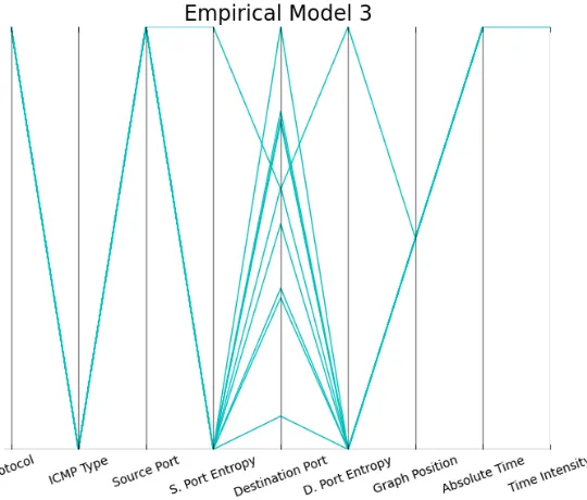
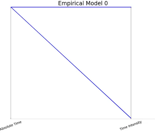
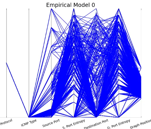
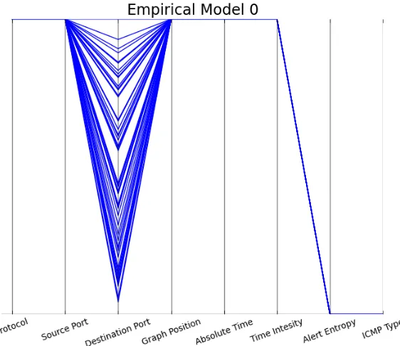
To work around this, a Python script was developed based on work done by [20] to generate parallel coordinate plots. These plots include multiple y-axis bars, one for each feature to be represented. The lines that connect between each feature bar aim to illustrate the diversity of a given feature. Figure 3.6 below shows an example for how these plots are used to represent the feature space of a given model.

From this example, the protocol of all samples in this model are the same since there is only one outgoing line from the ’Protocol’ axis. There is a lot of diversity seen in the destination ports of the samples which is seen by the spread of values throughout the ’Destination Port’ axis. In this case, it can be observed that the destination port entropy for this model is clearly stochastic while the source port entropy is deterministic. This is determined given that only one point on the ’Source Port’ axis connects to all other points in the ’Destination Port’ axis. Since the current working environment does not support the creation of these plots within the GUI of the tool, they are generated following the execution of the tool on a dataset based on files created during runtime. This ensures that the data is available for analysis regardless of the working environment the tool and framework are used in.

3.2

Algorithmic Changes

3.2.1 New Observables

The responsibility of a network is to pass packets containing data between different machines that are connected. While packets are the main form of observable data that can be analyzed to determine malicious behaviors, other forms of data and metadata exist from sensors and tools that help to monitor these networks. Intrusion Detection Systems (IDSs), such as Snort, monitor network traffic and search for packets that match known configurations of malicious activities. When an IDS finds a packet that matches a malicious action, an alert is produced that flags the packet and shows what malicious action it believes is being performed. These alerts are saved to log files that can be reviewed and analyzed by a system administrator or a network analyst. Figure 3.7 below shows an example of how the alert information from Snort is stored. Different formats are available, but the Snort fast alert style is commonly used to store this information.

Figure 3.8: Example of Bro Log

This information can be used to further describe traffic behavior observed on a network. An alert, depending on the IDS that produced it, contains additional information like the string identifying the alert type, the classification of the alert and a session number or iden-tification. Unfortunately, the only consistent information between different IDS files is the packet that triggered the alert and the string describing the action matched. It is important to note that the different IDS sources are used strictly to accommodate varying versions of metadata, not to compare the performance from utilizing different intrusion detection systems. Figure 3.8 above shows a log file generated from the Bro IDS. The Bro system produces several various log files while processing data. Each file contains different infor-mation about the data such as the HTTP log describing all HTTP based traffic seen and the weird log containing descriptions about abnormal patterns in the traffic. The format of the file and the information available is much different than what is given in Figure 3.7. To maintain consistency between different IDS metadata sources, the alert strings are encap-sulated with the packet level data that generated them to create a new form of observable information. In the dataset utilized, packets that generated alerts were filtered out of the packet capture files. When an alert file is specified, the tool will now reconstruct the traffic stream chronologically from both input sources. With the data reassembled, the overall account of behaviors that transpired on the network can be better observed.

Figure 3.9: Bro Log Processed into a CSV File

Figure 3.10: Snort Alerts Processed into a CSV File

Using built-in tools allow for quicker file operations and better portability between dif-ferent working environments. Interfacing with a MySQL database requires the use of the SQLAlchemy application programming interface (API) within the framework. When us-ing third party libraries, different release versions may not necessarily be available for each potential working environment. Interfacing with these additional libraries requires more complex configuration software and increased error handling. This increase in complex-ity is needed to prevent the program from terminating unexpectedly due to incidents such as a disconnect from the database software employed. Following the implementation of these modifications to the input data path, the framework is now scalable to handle large volumes of continuous data. Figure 3.11 below summarizes the updates made to the data input stream that is fed into the framework for processing. The highlighted area within the figure represents the changes made to the process flow of the system.

3.2.2 New Features

Feature selection for a machine learning framework is important for achieving the best possible performance. In a supervised machine learning setting, the data has labels that can help determine which features are relevant. In an unsupervised system, such as the darknet analysis framework, feature selection is particularly difficult as there are no labels to help determine strong features to describe the data. Dy et al. in [9] discuss the importance of finding strong features to use for unsupervised machine learning tools. Intuitively, all of the information available seems appropriate to use to try to describe the data. Unfortunately, this notion is not always correct as features may be redundant or irrelevant to the dataset. If a feature is irrelevant, then it may be difficult to distinguish the different clusters in a dataset as the data may overlap in the feature space. A redundant feature is one that does not add any value to the system. An example of this is when multiple clusters can be easily distinguished by one feature while other features fail to describe new dimensions in the feature space. It is important to identify unique dimensions in the feature space that add value to the classification system.

Table 3.1: Previously Implemented Features [20]

Feature Description Equation Protocol

A simple, discrete feature that represents the communication method between two

nodes.

P(P) = PN

i=1IP(xi)

N

ICMP Type

A discrete feature which represents simple packets that may be maliciously performing information reconnaissance

to identify a target and learn about potential weaknesses.

P(I) = PN

i=1II(xi)

N

Port Entropy

Examines the source and destination ports in a packet to see if they are deterministic or stochastic. Steady use of

a port usually means a service under attack while use of varying ports may

indicate reconnaissance actions.

P(P) =P(S)+ P(P|D)∗P(D)

Graph Position

How close a particular node is to other nodes with a high probability of being in

a malicious path within the same attack behavior model.

GP(i) =X j∈G

P(M|P_i,j0 )P(M|P_i,j−1) P

k∈Pi,j

1

P(M|Pk i,j)

The first entry in Table 3.1 above describes the equation used to calculate the probability of seeing protocolP in a given attack model. This is calculated with the indicator function

IP to count the percentage of protocol P in a given model M. The percentage is based on the total number of samples observed N and each individual element is described by

xi. Entry two uses the same concept to calculate the probability that a given ICMP TypeI

exists within a model. The port entropy of a model is given in entry three which describes the simplified equation used to compute the probability of a port value P. Given both the percentage of the port number and the “randomness” of all port values seen in the model the probability of seeing any given value P can be computed. The entropy is broken up into the probability of the values being stochastic or P(S) and the probability that it is deterministicP(D). These values are found by statistical bootstrapping with replacement and counting the number of deterministic values. The probability of a port value given that the ports within the model vary or P(M|S)is not calculated because the given port does not matter if they are being chosen randomly. To find the probability of the model given that it is deterministic or P(M|D) is found in the same manner of the previous features, finding the percentage of the value within the modelM.

The final row in the table describes the formula used to calculate the position of a given nodeiin the overall attack social graph. Finding the graph position is based on the concept of closeness centrality or how close a node is to any other given node. The numerator describes the weight of the starting hopP(M|P0

i,j)and ending hopP(M|P

−1

total path from nodeito nodej given asPi,j. This value will be higher if the path between

the two nodes stays within a given model M. The denominator represents the distance calculation of a given hop P(M|P_i,jk) within the total path. This represents the inverse harmonic mean of distances from nodeito all other nodes within the graph G. Nodes that are part of the same attack model with higher probability will contribute more towards the position calculation than those that are further away in the graph or span multiple models.

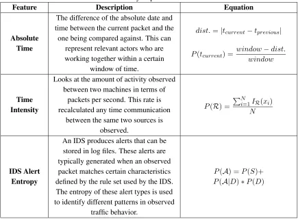
Table 3.2: Newly Implemented Features

Feature Description Equation

Absolute Time

The difference of the absolute date and time between the current packet and the

one being compared against. This can represent relevant actors who are working together within a certain

window of time.

dist.=|tcurrent−tprevious|

P(tcurrent) =

window−dist. window

Time Intensity

Looks at the amount of activity observed between two machines in terms of

packets per second. This rate is recalculated any time communication

between the same two sources is observed.

P(R) = PN

i=1IR(xi)

N

IDS Alert Entropy

An IDS produces alerts that can be stored in log files. These alerts are typically generated when an observed packet matches certain characteristics defined by the rule set used by the IDS. The entropy of these alert types is used to identify different patterns in observed

traffic behavior.

P(A) =P(S)+ P(A|D)∗P(D)

3.2.2.1 Absolute Time

in time increases between the time the packet was captured at and the time the behavior was first observed. The theory of dynamic time warp (DTW) was used as a basis for this feature..

The concept of DTW was used to mathematically model this feature. Dynamic time warping is a metric used to measure the similarity between two sequences despite vari-ances in speed or time. Bean in [1] discussed DTW and other methods like the longest common subsequence (LCS) algorithm as possible solutions to analyze the similarity of different attack tracks over time. DTW can also be utilized in other domains such as signa-ture verification. Mohammadi in [16] used this concept to match important points between two signatures to identify legitimate and forged samples. In this case, the DTW method was sufficient as the Euclidean distance formula is employed to calculate the cost, or dis-tance, between any two points in the tracks being compared.

A matrix describing the distance between every possible set of points in the two tracks is created using the Euclidean distance formula (3.1) below. In the equation, ai represents

an element in track a to be compared with bi which represents a corresponding element

within trackb.

d(a, b) =

v u u t N X i=1

(ai−bi)2 (3.1)

Once the matrix of costs is calculated, a continuous path, or warping path, is constructed from the starting point (1,1) to the opposite corner of the matrix (n, m). The optimal warped path is one that minimizes the distance between all shared points between the tracks being analyzed. Equation (3.2) below, as stated by [1], describes the methodology behind the algorithm to find the minimal warping path. Essentially, the dynamic time warping between a sequence A and a sequence B is given by the minimum path w where wi is

theith element in the warping path being considered and K is the normalization factor to account for sequences of different lengths [1].

DT W(A, B) =min w

 

 q

PK i=1wi

K (3.2)

With this feature, the similarity between time stamps of packets is not helpful in deter-mining how likely a given packet is to be part of an attack behavior. Instead, the behavior model that has the minimal distance in time to the packet being evaluated is the most likely behavior that characterizes the packet. Revisiting the Euclidean distance formula given by (3.1), the values of a andb would become the time of the current packet tcurrent and the

time of the most recent packet to be classified with the behavioral model being compared

tτ. Since the only dimension being investigated is time, the output of Equation (3.1)

be-comes the absolute value of the difference in time between two packets. Equation (3.3) below represents the revised mathematical representation of the absolute distance in time between two packets.

The distance in time is not enough by itself to describe a packet’s likelihood of being part of an attack behavioral model. To measure the probability that a packet belongs to a specific behavior, a relevancy window needs to be predefined. This window in time is different for each dataset used and values that fall outside of this window have zero probability for belonging to a given model. Given a frame of reference, the value calculated by (3.3) can be divided by the value for the time window to determine the probability of this packet belonging to a behavioral model.

Using the straight value of distance over the defined window space gives the opposite probability of the desired value. As the distance in time increases, the probability would increase that the packet belonged to that model. To fix this, the inverse of this value is used to decay the probability as the distance increases. Equation (3.4) below describes the probability equation where d is the value calculated from (3.3) and wis the value set for the relevancy window.

P(tcurrent) = 1−

d(tcurrent, tτ)

w (3.4)

Alternatively, (3.4) can be represented as one unified fraction as seen in Equation (3.5) below.

P(tcurrent) =

w−d(tcurrent, tτ)

w (3.5)

With this equation, it is possible to determine the likelihood of a packet belonging to a given attack behavioral model. The probability decays linearly as the distance increases between the time of the current packet and the time of the packet most recently incorporated into the attack model being evaluated.

For the iCTF2008 dataset, packets are time stamped with the UNIX epoch time they were captured at which is measured in seconds. Since traffic was observed frequently due to each of the teams working quickly to compromise different resources on the network, the times of the observed packets do not show much variance. The relevancy windowwchosen for this dataset was 120 seconds. Participants would likely try many different techniques to learn the network topology and exploit resources to capture flags during the eight hours alloted to play the game and score points. Two minutes seemed to be a reasonable time frame to isolate the time needed to capture fast scans and other techniques that teams might utilize during the game.

3.2.2.2 Time Intensity

frame resulting in much higher packet rates.

An example of a slow moving attack would be the SlowLoris attack. This is a type of denial of service (DoS) attack in which a program attempts to keep as many connections open to the victim machine as possible. This is accomplished by sending partial requests periodically to the target machine where the request is expanded on, but never completed. The end result is that the target machine exhausts its pool of connections preventing others from accessing its resources. These types of attacks are also difficult to detect as the pack-ets engaging the target often mirror legitimate traffic [6].

A smurf attack is another example of a way to cause a DoS. During a smurf attack, a malicious user sends an Internet Control Message Protocol (ICMP) echo request to a broad-cast domain such that all computers on the domain send ICMP echo replies. Normally, this procedure is used by routers to test the reachability of a machine on the network. In this case, the source address is spoofed to be the address of the target machine. By spoofing the target machine’s address, the influx of ICMP echo reply messages will consume band-width allocated to the victim and cause a DoS to legitimate users [14]. These two examples demonstrate how two attacks can have the same end result, but produce drastically differ-ent behaviors. The SlowLoris attack accomplishes a DoS through a slow consumption of resources while a smurf attack tries to consume bandwidth by sending a large volume of messages as quickly possible. These behaviors are distinct and should be distinguishable based on the rate of traffic they produce, which is the intuition behind the Time Intensity feature.

To calculate the rate of traffic per second along an edge, the time stamp, source IP ad-dress and destination IP adad-dress are extracted from the current sample. The source and destination IP addresses identify the edge in the network that this sample belongs to while the time stamp is used later to calculate the rate of the edge. An edge is defined as the con-nection between two communicating nodes where a node is the IP address of a machine. A Python dictionary object is used to store the information for each edge. Since this feature is relative to when the edge is first observed, each entry in the dictionary file includes the ini-tial time the edge was created, the time of the most recently observed packet and a running count of the total number of packets seen since the initial time. Equation (3.6) describes how the packet rate on an edge is calculated.

EdgeRate= P acketCount

CurrentT ime−InitialT ime+ 1 (3.6)

What this equation describes is that the larger the packet count is over the current time window, the larger the packet rate over the edge will be. The additional1in the denominator acts as an offset to prevent a divide by zero error. In many cases, it is possible to receive multiple packets within the same second so the initial edge rate will be equal to the packet count until the next time interval that packets are received in.

behavior model. Since this is a discrete empirical feature, each entry in the histogram is a discretized range of packet rates. Once the maximum rate has been determined from the edges, the histogram is generated with buckets set to an adjustable size until the maximum value is encapsulated within one of the discrete buckets.

The size of the buckets is adjustable, but an initial value of 5 was used as a default rate to prevent groupings of higher traffic volumes with lower ones. The initial value proved to be an appropriate choice as some empirical models contained multiple edges. These edges consisted of lower rates near 1 packet per second and higher edge rates closer to 20 packets per second. Using the default value, bucket 0 contains packet rates 0 to 5 with bucket 1 holding rates 6 to 10 and so on. The first bucket encapsulates the packet rates that are less than 1 because they are less common than the other values, particularly with the iCTF2008 dataset in which a large volume of traffic was observed throughout the duration of the game.

P(R) =

PN

i=1IR(xi)

N (3.7)

Once the histogram is complete, Equation (3.7) above is used to determine the probability of the rate R for a given model. To accomplish this, Equation (3.7) counts the number of occurrences of the edge rate Rusing the indicator functionIR(xi)on allN edge rates

observed by the current model. The indicator function is simply used to find all occurrences ofRwithin the set of all edge rates of the attack model. Another way to conceptualize this process is the total number of edge rates in the histogram bucket thatRbelongs to divided by the total number of edge ratesN in the attack model being evaluated.

3.2.2.3 Alert Entropy

Alert Entropy is another discrete feature that looks at the “randomness” or variance in the alert values captured by the IDS within the network topology. The intuition behind this feature is derived from Strapp in [20], Saddodin in [19] and Valeur in [21]. Work centered around alert correlation efforts demonstrates the value of metadata from IDSs [1, 19, 21]. These values can help to provide a stronger overview of events that may have transpired on a network. The design of the framework already allows packets, and now alert values, to be correlated in a graphical sense by connecting behavioral models together based on having relevant paths to the target of interest specified by the user.

actions. If an attack were to scan available ports on a victim machine, the variation of the destination ports would appear to be stochastic as no particular service is being targeted.

Combining the idea of feature entropy with the newly added alert data allows for a new metric to identify attack behaviors. Similar to the previously implemented Port Entropy feature, alerts can describe both stochastic and deterministic actions against a target ma-chine. Figure 3.12 below shows a sample from a Snort Alert file showing a deterministic attack type being executed against a target machine. It can be seen that the same target is attacked by the same source with the same attack type, as described by the alert string.

Figure 3.12: Example of Deterministic Alert Behavior

This set of alerts is consistent with buffer overflow exploits in Transmission Control Protocol (TCP) traffic [18]. A buffer overflow attack is where an attacker will purposefully write information beyond the defined bounds of a memory segment, or buffer, such that a variable, pointer or return address will be changed [2]. If a remote user is successful in changing any one of these fields, the flow of the program can be altered. An example of this exploit would be a login program where an attacker would overrun the buffer storing the password hash of a benign user. The attacker would then supply their password when prompted along with additional characters followed by the hash of their password. These extra characters will overrun the buffer used by the program and inject the hash of the attacker’s password in the space normally reserved for storing the hash of the benign user’s password. This would cause the program to hash the attacker’s password and compare it to the hash injected by the buffer overflow, granting the attacker access to the target machine [2].

Figure 3.13: Example of Stochastic Alert Behavior

different techniques to try to gain access to the target machine through this application as described by the alert strings.

These examples demonstrate the validity of using the entropy of a feature as originally proposed by [20]. The same intuition that was applied to ports from packet headers can be applied to the alert strings found within the files generated by Snort. Since strings are typically more difficult to process and typically require more computation time than num-bers, the built-in hash function native to Python was used to convert each alert string into an integer. Hashing the alert string also requires less memory to store the value making it less taxing on system resources. Once hashed, this allows for the use of the original port entropy equation as developed by [20] with the alert integer values as given below by Equation (3.8).

P(A) =P(A|S)P(S) +P(A|D)P(D) (3.8)

This equation states that the probability of a given alert value is equivalent to the prob-ability of the alert value being trigged with a stochastic behavior plus the probprob-ability of the alert value appearing given a deterministic behavior. Statistical bootstrapping is used to determine the value ofP(D), the probability of a deterministic behavior, and the value ofP(S), the probability of a stochastic behavior [20]. Statistical bootstrapping consists of random sampling from the total set of samples, with replacement, to determine the total occurrences of stochastic and deterministic samples. As seen in Figure 3.13, the specific value of the alert string is less relevant when a myriad of malicious techniques are utilized to exploit a vulnerability in a target. This means that the probability of an alert string appear-ing due to a stochastic behavior, P(A|S), is unimportant as any value is equally probable because each observation is treated as independent and identically distributed (i.i.d.) by the classifier. As this observation matches that of the Port Entropy feature, it is appropriate to use the reduced form of Equation (3.8).

P(A) = P(S) +P(A|D)P(D) (3.9)

Equation (3.9) above illustrates the reduced equation used to represent the Alert Entropy feature.

3.2.3 Revision of the Model Introduction Strategy